HAL Id: hal-01118324
https://hal.inria.fr/hal-01118324
Submitted on 18 Feb 2015
HAL is a multi-disciplinary open access
archive for the deposit and dissemination of
sci-entific research documents, whether they are
pub-lished or not. The documents may come from
teaching and research institutions in France or
abroad, or from public or private research centers.
L’archive ouverte pluridisciplinaire HAL, est
destinée au dépôt et à la diffusion de documents
scientifiques de niveau recherche, publiés ou non,
émanant des établissements d’enseignement et de
recherche français ou étrangers, des laboratoires
publics ou privés.
Real Time Semi-dense Point Tracking
Matthieu Garrigues, Antoine Manzanera
To cite this version:
Matthieu Garrigues, Antoine Manzanera. Real Time Semi-dense Point Tracking. ICIAR, 2012, Aveiro,
Portugal. pp.245 - 252, �10.1007/978-3-642-31295-3_29�. �hal-01118324�
Matthieu Garrigues and Antoine Manzanera
ENSTA-ParisTech, 32 Boulevard Victor, 75739 Paris CEDEX 15, France,
http://uei.ensta.fr
matthieu.garrigues@ensta-paristech.fr antoine.manzanera@ensta-paristech.fr
Abstract. This paper presents a new algorithm to track a high number of points in a video sequence in real-time. We propose a fast keypoint detector, used to create new particles, and an associated multiscale de-scriptor (feature) used to match the particles from one frame to the next. The tracking algorithm updates for each particle a series of appearance and kinematic states, that are temporally filtered. It is robust to hand held camera accelerations thanks to a coarse-to-fine dominant movement estimation. Each step is designed to reach the maximal level of data par-allelism, to target the most common parallel platforms. Using graphics processing unit, our current implementation handles 10 000 points per frame at 55 frames-per-second on 640 × 480 videos.
1
Introduction
Estimating the apparent motion of objects in a video sequence is a very useful primitive in many applications of computer vision. For fundamental and practical reasons, there is a certain antagonism between reliability (are we confident in the estimated velocities) and density (is the estimation available everywhere). Then one has to choose between sparse tracking and dense optical flow. In this paper we propose an intermediate approach that performs a long term tracking of a set of points (particles), designed to be as dense as possible. We get a flexible motion estimation primitive, that can provide both a beam of trajectories with temporal coherence and a field of displacements with spatial coherence. Our method is designed to be almost fully parallel and then extremely fast on graphics processing unit (GPU) or multi-core systems.
Our work is closely related to the Particle Video algorithm of Sand and Teller [5], with significant differences: we use temporal filtering for each particle but no explicit spatial filtering, and our method is by design real-time. Since the pioneering work of Tomasi and Kanade [8], there have been different real-time implementations of multi-point tracking, e.g. Sinha et al [6], and Fassold et al [2]. There are also real-time versions of dense and discontinuities preserving optical flow, e.g. d’Angelo et al [1]. However these techniques do not provide the level of flexibility we are looking for. In a recent work [7], Sundaram et
2
al achieved an accelerated version on GPU of a dense point tracking, which combines density and long term point tracking. In their work, a subset of points are tracked using velocities obtained from a dense optical flow. Although quite fast, their parallel implementation spend more than half of the computation time for the linear solver, which is at the core of the spatial regularisation needed by the dense optical flow. Our work is based on the opposite approach: tracking -as individually -as possible - the largest number of points, in order to get the semi-dense optical flow field by simple spatial filtering or expansion.
The contributions of our work are the following: (1) a fast multiscale detector which eliminates only the points whose matching will be ambiguous, providing the semi-dense candidate particle field, (2) a method for detecting abrupt ac-celeration of particles and maintain the coherence of the trajectories in case of sudden camera motion change, (3) a real-time implementation, (4) a spatial co-herence which is not enforced by explicit spatial filtering but only used as part of a test to reject unreliable particle matching, and (5) an objective evaluation measure allowing online validation and parameter tuning without ground truth. The paper is organised as follows: Section 2 describes the weak keypoint detector used to select the new candidate particles, and defines the feature de-scriptor attached to them. Section 3 presents the tracking algorithm. Section 4 gives some details of the parallel implementation and presents the execution time. Finally Section 5 presents our online evaluation method and discusses the quality of results.
2
Feature point selection
2.1 Weak keypoint detection
The first step aims to select the points that we can track through the video sequence. The goal is to avoid points that can drift, typically on flat areas, or on straight edges. Our detector is based on the idea that the matching of one pixel p can not be determined at a certain scale, if there exists a direction along which the value varies linearly at the neighbourhood of p. This is precisely what the following saliency function calculates.
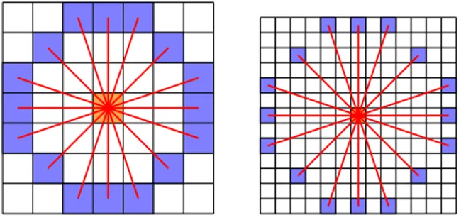
Let Br(p) denote the set of 16 pixels evenly sampled on the Bresenham circle
of radius r centred on p (see Fig. 1). I is the current video frame with gray level values in [0, 1]. Let the local contrast be κr(p) = maxm∈Br(p)|Ir(p) − Ir(m)|
with Ir the image I convolved with the 2d Gaussian of standard deviation σr.
Let {m1, . . . , m16} denote the pixels of Br(p), numbered clockwise. To evaluate
Cr(p), the saliency of p at one scale, we search for the minimum deviation from
linearity of the function I along the diameters of Br(p):
Sr(p) =
1
2i∈[1,8]min |Ir(mi) + Ir(mi+8)− 2Ir(p)| .
Cr(p) = ( 0 if κr(p) < µ Sr(p) κr(p) otherwise .
Normalisation by κr(p) makes Cr contrast invariant and thus allows
extrac-tion of keypoints even in low contrast areas. The multiscale saliency of p is finally defined as: C(p) = max
r Cr(p).
Since we need the highest possible number of particles to feed a massively parallel processor, we set the threshold µ to the lowest possible value. On our test videos with gray level pixel values in [0, 1], we used µ = 0.02. We used two radii r ∈ {3, 6}, with σ3= 1.0 and σ6= 2.0.
Finally, the detector creates new particles if the two following criteria hold: 1. C(p) ≥ β .
2. ∀n ∈ c9(p), C(p) ≥ C(n) .
3. No particle already lives in c9(p) .
c9(p) denotes the 3 × 3 neighbourhood of p. (1) discards non trackable points.
(2) promotes local maxima of C, and (3) ensures that two particles do not share the same location. β = 0.25 in our implementation.
Our detector is similar to the FAST detector [4]. In fact, while meeting our real-time requirements, it is slightly slower than FAST since it involves more value fetches. But it is more adapted to our needs, being weaker in the sense that it detects a much higher number of points.
Fig. 1.The two neighbourhoods B3 and B6.
2.2 Good (enough) feature to track
The detected keypoints will be tracked using a feature vector computed on each pixel of the video frame. For real-time purposes, it must be fast to compute, small in memory, and robust just enough to handle changes between two consecutive frames.
In this paper we simply used as feature vector 8 values evenly sampled from the Bresenham circles at each scale used to calculate the saliency function (see Fig. 1). Then using B3and B6we get a 16 dimension (128 bits) feature vector.
Note that the keypoint detector and feature extraction functions are merged. In the following, two feature vectors will be compared using the normalised L1 distance, which is computationally efficient and sufficient to find the most
4
3
Tracking Algorithm
The goal of the tracking algorithm is to follow particle states through the video frames. We present in this section a multi-scale approach robust to large hand held camera acceleration.
3.1 Multiscale particle search and update
A particle i is a point tracked over the video sequence. Its state at frame t holds its appearance feature ft(i) (See Section 2.2), velocity vt(i) in the image plane
and age at(i) (i.e. the number of frame it has been tracked). We update these
attributes at each input frame. We also compute the instantaneous acceleration w, but do not keep it in the particle state. Instead, we record the values of w in a histogram, and compute the mode to estimate the dominant acceleration.
Our method builds a 4 scales pyramid of the input and tracks particles at each scale by making predictions about their probable neighbourhood in the next frame. Psis the set of particles tracked at scale s. We apply the following
coarse to fine algorithm:
M4← (0, 0)
for scale s ← 3 to 0:
| initialise every bin of the histogram H to 0. | foreachparticle i ∈ Ps
| | pˆt(i) ← pt−1(i) + st−1(i) + 2Ms+1[Prediction]
| | pt(i) ← Match( ˆpt(i), ft−1(i)) [Matching]
| | if dL1(ft−1(i), F (pt(i))) > γ then delete i
| | else
| | ft(i) ← ρF (pt(i)) + (1 − ρ)ft−1(i)
| | vt(i) ← ρ(pt(i) − pt−1(i)) + (1 − ρ)vt−1(i)
| | at(i) ← at−1(i) + 1
| | w← pt(i) − pt−1(i) − vt−1(i)
| | H(w) ← H(w) + 1 | endfor | if s >0 | Ms ← arg max x H(x) | else | Ms ← 2Ms+1 | foreachparticle i ∈ Ps | | vt(i) ← vt(i) − ρM s | endfor
| create new particles at scale s | foreachnewly created particles i ∈ Ps
, s <3
| | search a particle n with at(n) > 1 in a 5x5 neighbourhood at scale s + 1
| | if nis found | | vt(i) ← 2vt(n)
| endfor endfor
Match(p, f ) only searches in the 7x7 neighbourhood of ˆpt for the position
of the closest feature to f given the L1 distance in the feature space (See Sec.
2.2). If the match distance is above the threshold γ, we consider the particle lost. Given that 0 < dL1(x, y) < 1, we set γ = 0.3 to allow slight appearance
change of particles between two frames. The algorithm predicts particle position at scale s using their speed and Ms+1, the dominant acceleration due to camera
motion. Ms is initially set to (0, 0) and refined at every scale s > 0. We then
subtract ρMs to the particle velocities to improve the position prediction at
the next frame. The parameter ρ smoothes velocity and feature over the time. In our experiments, we use ρ = 0.75. It is worth mentioning that although the tracker maintains a pyramid of particles, there is no direct relations between the particles at different scales, except for newly created particles, that inherit velocity from their neighbours at upper scale. The particles of scales larger than 0 are only used to estimate the dominant motion, which is essential to get a good prediction at scale 0 (highest resolution).
3.2 Rejecting Unreliable Matches
When an object gets occluded, or change appearance, some wrong matches oc-cur and usually implies locally incoherent motion. Thus, for each particle i, we analyse a 7x7 neighbourhood to count the percentage of particles that move with a similar speed. If this percentage is less than 50%, i is deleted. Note that this method fails to detect unreliable motion of isolated particles (where the neighbourhood does not contain other particles).
4
GPU implementation
For performance reasons, we store the set of tracked particles in a 2D buffer G such as G(p) holds the particle located at pixel p. Then, particles close in the image plane will be close in memory. Since neighbour particles are likely to look for their matches in the same image area, this allows to take advantage of the processor cache by factorising pixel value fetch. This also adds a constraint: One pixel can only carry one particle. Thus, when two particles converge to the same pixel, we give priority to the oldest. We track particles at different scales with a pyramid of 2D particle maps.
To take maximum advantage of the GPU, the problem has to be split into several thousands of threads in order to hide the high latency of this architecture. Applications are generally easier to program, and execute faster if they involve no inter-thread communication. In our implementation, one thread individually processes one pixel. This allows fast naive implementation of our algorithm.
Our current implementation uses the CUDA programming framework [3]. We obtain the following performances using a 3 Gz quad-core CPU (intel i5-2500k, 2011) and a 336-cores GPU (NVIDIA Geforce 460 GTX, 2010). At full resolution (640 × 480) the system can track about 10 000 particles at 55 frames per second. Table 1 shows running times of each part of the algorithm.
6
5
Evaluation and Results
Evaluation of a tracking algorithm in a real world scenario is not straightforward since it is difficult to build a ground truth containing the trajectories of every points of a given video. We propose in this section measurements that provide objective quantitative performance evaluation of the method.
A tracking algorithm typically makes two types of errors:
(A) When a particle dies while the scene point it tracks is still visible, reducing the average particle life expectancy.
(B) When a particle jumps from one scene point to another similar but different. It usually causes locally incoherent motion.
We base our evaluation on two facts: In our test videos, scene points generally remain visible during at least 1 second, and objects are large enough to cause locally coherent particles motion. Thus, the quality of the algorithm is directly given by the average live expectancy of particles, the higher the better, and the average number of rejected matches (See Sec. 3.2) by frame, the lower the better. We also compute the average number of tracked particles on each frame. It has to be as high as possible, keeping in mind that creating too many irrelevant particles may increase the proportion of errors A and B.
Table 2 shows the quality measures of the results obtained with our current implementation on three videos: Two (VTreeTrunk and VHall) made available by Peter Sand and Seth Teller from their works on particle video [5]. These videos are taken from a slowly moving subject. And another one (HandHeldNav) taken from a fast moving hand-held camera where points are harder to track since the camera undergoes abrupt accelerations, causing large translations and motion blur. Scale 4 3 2 1 Keypoint + feature 0.08 0.27 0.92 3.47 Particle creation 0.01 0.03 0.08 0.31 Matching 0.13 0.23 0.88 3.09 Global movement 0.21 0.37 1 X Rejected matches 0.05 0.09 0.31 1.16 Table 1. Running times (in milliseconds) of the different parts at the 4 scales on video HandHeldNav. Those timings were obtained using the NVIDIA Visual Profiler.
VTree VHall HandHeld Life expectancy 32.1 24.5 15.6 Rejected matches 134 22 351 Alive particles 25770 4098 9327 Table 2. Evaluation measures of our method on the three videos: Average life expectancy of particles on the whole video, average rejected matches per frame, and av-erage number of particles per frame.
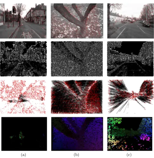
Figure 2 shows qualitative results of our experiments. It displays the particles, their trajectories, the optical flow computed from particle velocities and saliency function in different scenarios.
(a) (b) (c)
Fig. 2. Experimental results at fine scale on 3 different scenarios. First row shows the current video frame with particles older than 10 frames in red. Second row is the saliency function C. Third row draws a vector between the current position of each particle and its birth position. Fourth row represents the reconstructed semi-dense optical flow using particle velocities. At pixels where no particle lives, we approximate the flow using the velocities of the neighbour particles if their gray level is similar. (a) Static camera, moving objects; (b) Circular travelling, static objects; (c) Forward zoom, moving objects.
6
Conclusion
We proposed a new approach to track a high number of keypoints in real-time. It is robust to hand held camera acceleration thanks to a coarse to fine dominant movement estimation. This provides a solid and fast building block to motion es-timation, object tracking, 3D reconstruction, and many other applications. Each particle individually evolves in the image plane by predicting its next position,
8
and searching the best match. This allows to split the problem into thousands of threads and thus to take advantage of parallel processors such as a graphics processing unit. Our current CUDA implementation can track 10 000 particles at 55 frames-per-second on 640 × 480 videos.
In future works, we wish to apply this primitive in several applications of mobile video-surveillance. For the real-time aspects, we will perform a deeper analysis of the parallel implementation. To be able to address a larger number of scenarios, we will also study the extension of the dominant motion estimation to other acceleration cases, in particular rotation.
Acknowledgements
This work takes part of a EUREKA-ITEA2 project and was funded by the French Ministry of Economy (General Directorate for Competitiveness, Industry and Services).
References
1. d’Angelo, E., Paratte, J., Puy, G., Vandergheynst, P.: Fast TV-L1 optical flow for interactivity. In: IEEE International Conference on Image Processing (ICIP’11). pp. 1925–1928. Brussels, Belgium (September 2011)
2. Fassold, H., Rosner, J., Schallaeur, P., Bailer, W.: Realtime KLT feature point tracking for high definition video. In: Computer Graphics, Computer Vision and Mathematics (GraVisMa’09). Plzen, Czech Republic (September 2009)
3. NVIDIA: Cuda toolkit, http://www.nvidia.com/cuda
4. Rosten, E., Drummond, T.: Machine learning for high-speed corner detection. In: European Conference on Computer Vision (ECCV’06). vol. 1, pp. 430–443 (May 2006)
5. Sand, P., Teller, S.: Particle video: Long-range motion estimation using point tra-jectories. In: Computer Vision and Pattern Recognition (CVPR’06). pp. 2195–2202. New York (June 2006)
6. Sinha, S.N., Frahm, J.M., Pollefeys, M., Genc, Y.: Feature tracking and matching in video using programmable graphics hardware. Machine Vision and Applications 22(1), 207–217 (2007)
7. Sundaram, N., Brox, T., Keutzern, K.: Dense point trajectories by GPU-accelerated large displacement optical flow. In: European Conference on Computer Vision (ECCV’10). pp. 438–451 (September 2010)
8. Tomasi, C., Kanade, T.: Detection and tracking of point features. Carnegie Mellon University Technical Report CMU-CS-91-132 (April 1991)