HAL Id: inria-00541778
https://hal.inria.fr/inria-00541778
Submitted on 1 Dec 2010
HAL is a multi-disciplinary open access
archive for the deposit and dissemination of
sci-entific research documents, whether they are
pub-lished or not. The documents may come from
teaching and research institutions in France or
abroad, or from public or private research centers.
L’archive ouverte pluridisciplinaire HAL, est
destinée au dépôt et à la diffusion de documents
scientifiques de niveau recherche, publiés ou non,
émanant des établissements d’enseignement et de
recherche français ou étrangers, des laboratoires
publics ou privés.
Incremental Local Online Gaussian Mixture Regression
for Imitation Learning of Multiple Tasks
Thomas Cederborg, Ming Li, Adrien Baranes, Pierre-Yves Oudeyer
To cite this version:
Thomas Cederborg, Ming Li, Adrien Baranes, Pierre-Yves Oudeyer. Incremental Local Online
Gaus-sian Mixture Regression for Imitation Learning of Multiple Tasks. IEEE/RSJ International Conference
on Intelligent Robots and Systems (IROS 2010), 2010, Taipei, Taiwan. �inria-00541778�
Incremental Local Online Gaussian Mixture Regression for Imitation
Learning of Multiple Tasks
Thomas Cederborg, Ming Li, Adrien Baranes and Pierre-Yves Oudeyer
Abstract— Gaussian Mixture Regression has been shown to be a powerful and easy-to-tune regression technique for imitation learning of constrained motor tasks in robots. Yet, current formulations are not suited when one wants a robot to learn incrementally and online a variety of new context-dependant tasks whose number and complexity is not known at programming time, and when the demonstrator is not allowed to tell the system when he introduces a new task (but rather the system should infer this from the continuous sensorimotor context). In this paper, we show that this limitation can be addressed by introducing an Incremental, Local and Online variation of Gaussian Mixture Regression (ILO-GMR) which successfully allows a simulated robot to learn incrementally and online new motor tasks through modelling them locally as dynamical systems, and able to use the sensorimotor context to cope with the absence of categorical information both during demonstrations and when a reproduction is asked to the system. Moreover, we integrate a complementary statistical technique which allows the system to incrementally learn various tasks which can be intrinsically defined in different frames of reference, which we call framings, without the need to tell the system which particular framing should be used for each task: this is inferred automatically by the system.
I. INTRODUCTION
The paper examines the question of how to create robots able to learn incrementally and online a variety of new context-dependant tasks whose number and complexity is not known at programming time, and when the demonstrator is also not allowed to tell the system how many tasks there are and whether a given demonstration corresponds to a variation of an already demonstrated task or to a new tasks. Moreover, the demonstrator may alternate demonstrations correspond-ing to different tasks in an uncontrolled or even random order. Yet, we assume that elements of the sensorimotor context can allow the robot to statistically infer information that may allow it to accurately reproduce the right task in a given sensorimotor context.
Like the approach presented in this paper, this does not necessarily rely on an explicit segmentation or clustering of demonstrations. The proposed approach incrementally and locally models the set of all tasks as a single dynamical system. Different tasks just correspond to different regions of the state space and the thing that changes between different tasks is the part of the state that continuously (as opposed to symbolically or categorically) models the sensorimotor context.
Imitation Learning and related work: Before presenting our system, we shall quickly review related work. There are two primary goals in the field of imitation learning
This research was partially funded by ERC Grant EXPLORERS 240007
(sometimes referred to as Programing by Demonstration (PbD) or Robot programing by Demonstration(RbD)). The first is to study how social learning works in humans and the second is to see how social learning can work in general and how to build better artifacts using this knowledge. Four central questions were defined in [9] as what, how, when and who to Imitate. In this paper, we focus on aspects of the what and how questions and our aim is targeted towards the building of robots that can efficiently and flexibly learn by demonstration.
One approach is to define a set of primitive behaviors or actions and segment the problem into several different sub problems. Learning how to reproduce these individual behav-iors, finding a way to classify parts of a demonstration as a series of behaviors and finding an algorithm that can learn from a demonstration when described as a list of behaviors, including how to generalize to new situations using this list, can here be decomposed into related but separable problems. The task can be encoded using possibly hierarchical, graph based models, for example Hidden Markov Model, with parameters set using machine learning algorithms. Examples of this approach include [5] working with a wheeled robot and [6] and [7] which proposes to use a hierarchical model to encode household tasks such as setting the table. [8] encodes a demonstration using a set of pre defined postures, extracting task rules in the space of these postures. [8] also explores the question of granularity as it is necessary to decide if a given part of the task should be a primitive or composed of more finely grained primitives.
Another approach, which is not necessarily incompatible with the previous one, is to encode the demonstration at the trajectory level. Instead of building a model that operates on discrete primitive actions, this approach builds models that operates in continuous spaces, for example in the joint space of the robot or in the operational/task space, such as the position, speed or torque space of its hands, mapping sensory inputs to motor outputs or desired hand velocities (which can be seen as different levels of granularity). In the early work of [11] the set of acceptable trajectories is spanned by the trajectories seen during the demonstrations, and [12] introduces a non parametric regression technique based on natural vector splines to build a representation of a trajectory either in cartesian (sometimes referred to as task space) or joint coordinates, from several demonstrations. In [13] a method inspired by dynamical systems and attractors is presented using recurrent neural networks to learn different motions and switch between them. The mimesis model proposes to encode a trajectory as a Hidden Markov Model
HMM. Reproduction is achieved using a stochastic algorithm on the transition probabilities of the HMM.
Among these continuous trajectory-level approaches, Cali-non et al. showed, through a series of advanced robotic experiments [1], [14], [2], [15], that the Gaussian Mixture Regression technique, introduced in [22], could be very successfully and easily used for encoding demonstrations through a GMM tuned with an expectation-maximization algorithm [16], as well as for extracting their underlying constraints and reproducing smooth generalized motor tra-jectories. This approach alleviates much of the work from the programmers, who only need to find the number of gaussians for each task. Basically the same model can be used for a wide variety of tasks and robustly reproduces smooth movements. Once the model is built, and following for example the time-independant approach presented in [4], it can be queried quickly with the current state giving the desired action (minimizing the needed computation time once the model has been learnt). This is a very powerful method but it does have some limitations, which we will address in this paper, that prevent it from being directly used when one wants a robot to learn incrementally and online new tasks. This is especially true when the programmer does not know in advance the number and the complexity of tasks, and when the demonstrator is not allowed to provide categorical information about the demonstrations.
In the case of a single task (so that the number of gaussians does not have to be changed and there is no question of which task is demonstrated) a more incremental approach has been proposed in [14], but it still requires re computation of the model and it is not obvious how to extend it to the context of incorporating a demonstration of a new task within this framework. Indeed, in this approach to GMR when a new task is introduced, the number of gaussians should typically be increased manually by the programmer. Even if this is would be done automatically one would have to somehow inform the robot that the demonstration is of a new task and then wait for the entire model to be rebuilt after automatically discovering the number of gaussians, which becomes computationally exponentially more difficult as EM needs to tune the parameters of more and more gaussians in the mixture. What we would like is to have a demonstrator teach the robot a task and when he wants to start teaching the robot a completely different task (perhaps because the robot does the current task well or if the demonstrator does not think he is able to learn the current task), but avoiding any additional programmer intervention or global/heavy recomputation of a model. In this framework the robot needs to infer what task he is to perform based on the environment only. When a new task is to be taught, and the demonstrator would like the task to be executed in a particular situation, he simply sets up the environment and demonstrates the new task (the task to be reproduced is thus dependent on the environment). The robot stores both how the environment looks and what the demonstrator has shown him. The decision of what environment should produce a task is made by the demonstrator at the time of the first
demonstration of the task. This way there is no need for any additional intervention on the programming level or any need to pass some form of ”new task being demonstrated” symbol to the robot.
It would also be nice if a new demonstration could immediately be incorporated online and incrementally during the teaching process. To achieve these goals we introduce an Incremental, Local and Online formulation of Gaussian Mixture Regression (ILO-GMR). The central idea of this technique is to build online and on-demand local Gaussian Mixture Regression regression models of the task(s).
During training in this approach, data points are stored incrementally in a data structure which allows for very fast approximate nearest neighbors retrieval (e.g. such as in [21]). Then, at prediction/reproduction time, the method looks at the points in the database that are close to the current state of the system, including sensorimotor context information, and a local GMR model is built online. As the model is very local, only a few gaussians are needed (typically 2 or 3), and experimental results show that an EM and GMR with 2 or 3 gaussians and around 100 points can be run in a few milliseconds on a standard computer, which is enough for many real-time robot control setups. Thus, new data points from a demonstration, either of a task already seen or of a new task, can be exploited immediately without heavy recomputations and without any programmer intervention (standard parameters of ILO-GMR experimentally work for large number of tasks of varying complexity) giving us the advantages of a truly incremental and online algorithm.
II. ALGORITHM
A. Gaussian Mixture Regression
The GMR approach [1] first builds a model (typically in task space, but models in the joint space can also be used) using a Gaussian Mixture Model encoding the covariance relations between different variables. If the correlations vary significantly between regions then each local region of state space visited during the demonstrations will need a few gaussians to encode this local dynamics. Given the number of gaussians, the use of an Expectation Maximization (EM) algorithm finds the parameters of the model.
A Gaussian probability density function consists of a mean µ and a covariance matrix Σ. The probability density ρ of observing the output v from a gaussian with parameters µ andΣ is:
ρ(v) = 1
2π�|Σ|exp{− 1
2(v − µ)TΣ−1(v − µ)} (1) To get the best guess of the desired output (e.g. speed in cartesian space of the hand in the robot experiments below) ˆv given only the current state xq (e.g. position and speed
of the hand in various referentials and position of an object construing the context, as in the experiments below) we have: ˆv(xq) = E[v|x = xq] =µv+Σvx(Σxx)−1(xq− µx) (2)
WhereΣvx is the covariance matrix describing the
A single such density function can not encode non linear correlations between the different variables. To do this we can use more than one gaussian to form a Gaussian Mixture Model defined by a parameter list λ = {λ1,λ2,··· ,λM},
where λi= (µi,Σi,αi) and αi is the weight of gaussian i.
To get the best guess ˆv conditioned on an observed value xqwe first need to know the probability hi(xq) that gaussian
i produced xq. This is simply the density of the gaussian
i at xq divided by the sum of the other densities at xq,
hi(xq) =∑Mρi(xq)
j=1ρj(xq) (where each density ρi(v) is calculated
just as in (1), withΣ replaced by Σxx
i , v with xq, etc). Writing
out the whole computation we have: hi(xq) = αi √|Σxx i |exp{− 1 2(xq− µix)T(Σxxi )−1(xq− µix)} ∑M j=1√α|Σjxx j |exp{− 1 2(xq− µxj)T(Σxxj )−1(xq− µxj)} . (3) Given the best guesses ˆvi(xq) from (2), and the
probabili-ties hi(xq) that gaussian i generated the output, the best guess
ˆv(xq) is given by: ˆv(xq) = M
∑
i=1 hi(xq) ˆvi(xq) (4)The parameter list is found using an Expectation Maxi-mization algorithm (EM) [16] that takes as input the number of gaussians and a database.
B. Incremental Local Online Gaussian Mixture Regression (ILO-GMR)
With ILO-GMR, the datapoints of all demonstrations, possibly including demonstrations of different tasks, are stored in a full data structure D which allows later on for very fast approximate nearest neighbors queries. The datastructure we use is a kd-tree-like incremental variant of approximate nearest neighbors algorithm presented in [21] and already shown to be very efficient in high-dimensional computer vision applications. Then, during each iteration of the reproduction of a task the robot looks at his current state xq and extracts a local database D(xq) consisting of
the N points closest to xq using the fast query algorithm.
These points are now used as input to GMR as described above along with a number M of gaussians to use (typically equal to 2 or 3). N is the first parameter of ILO-GMR and is typically slighlty superior to the second parameter M multiplied by the dimensionality of the sensorimotor space. The EM algorithm builds a GMM and then we get the best guess of the current desired speed ˆv(xq,D(xq),N,M) as
described above. The local points are found online during reproduction and therefore it allows the system to take advantage of information it has just acquired as easily as old information available before task execution began.
The number of gaussians M and the number of local points N does not need to be changed when a demonstration of a new task is introduced and the modeling is done online. Thus we can add new demonstrations of old tasks or demonstrations of new tasks incrementally to the system without tampering with model parameters or recomputing a model. The pseudo-code of the algorithm is provided below.
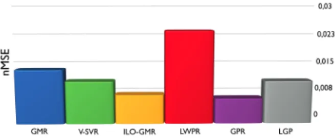
Computational complexity and ease-of-tuning An im-portant difference between the standard GMR approach and ILO-GMR is that in ILO-GMR an important part of process-ing is shifted from the trainprocess-ing period to online computation. Hopefully, since models in ILO-GMR are ”very local”, using only 2 or 3 gaussians will be enough for reaching high accuracy while allowing for very fast EM and local GMR steps. As far as the incremental training is concerned, [21] has shown that the datastructure for fast nearest neighbours retrieval could also be updated very fast. In order to make an initial experiment to evaluate ILO-GMR both in terms of accuracy for difficult robot-related regression tasks, as well as computational speed, we have compared the performance of ILO-GMR with other state-of-the-art regression methods, including GMR, on the hard regression task defined in the SARCOS dataset which has been used several times in the literature as a benchmark for regression techniques in robotics. This dataset encodes the inverse dynamics of the arm of the SARCOS robot, with 21 input dimensions (position, velocity and acceleration of 7 DOFs) and 7 output dimensions (corresponding torques). It contains 44484 ex-amplars in the training database and 4449 test exex-amplars. It is available at: http://www.gaussianprocess.org/gpml/data/). The regression methods to which we compared performances on this dataset are: Gaussian Mixture Regression (GMR, [1] and [22]), Gaussian Process Regression (GPR, [17]), Local Gaussian Process Regression (LGP, [19]), support vector regression (v-SVR, [20]) and Locally Weighted Projection Regression (LWPR, [18]). All those algorithms were tuned with reasonable effort to obtain the best generalization re-sults. For ILO-GMR, optimal tuning was done with N=200 and m=2, but results degrade very slowly when moving away from these parameters. Figure 1 shows the comparison of the performances of those algorithms for predicting the torques of the first joint in the SARCOS database. We observe that the performance of ILO-GMR matches nearly the best performance (GPR), is slightly better than v-SVR, LGP and GMR, and clearly better than LWPR while being also incremental but much easier to tune. Furthermore, in spite of the fact that our current implementation of ILO-GMR was done in Matlab and is not optimized, it is already able to make a single prediction and incorporate a new learning examplar in around 10 milliseconds on a standard laptop computer and when 44484 SARCOS data examples are already in memory. Furthermore, we have measured experimentally the evolution of training and prediction time per new examplar: it increases approximately linearly with a small slope in the range 0-44484 learning examplars. Finally, it can be noted that the parameters N and M can be chosen the same for the SARCOS database as for the various motor tasks demonstrated in the experiments presented below, in spite of the fact that they are defined in very different sensorimotor spaces: this illustrates the ease-of-tune of ILO-GMR.
Fig. 1. Comparison of ILO-GMR with state-of-the-art regression algo-rithms for the SARCOS dataset encoding the inverse dynamics of an arm with 21 input dimensions. Here, only the nMSE for the regression of the torque of the first joint is displayed.
C. How do we pick local points
A potential problem with the use of ILO-GMR in a number of robot learning by demonstration applications is that for given tasks there may be irrelevant or redundant or badly scaled variables defining the state xq that may cause
problems for generalization through the nearest neighbours search. We address these issues in this paragraph.
First, we do not want the importance of a dimension to be encoded in the size of its values so we rescale all the data so that every dimension has the same variance and mean zero. This rescaling uses the entire data set so adding new data means that the rescaling constants should ideally be updated: this can however be done quickly and incrementally. A global model is able to capture the relevant dimensions for every task in every region of the state space given that the number of gaussians are appropriate and that it has enough training data. We must make sure that this very important property of the global GMR algorithm is not lost in ILO-GMR. The way in which local points are selected correspond to an assumption about what dimensions are relevant to the task. To pick the local points from a dataset D with K number of dimensions d1,d2, ...,dK; we must
decide how we measure distance between two points p1=
(x11,x12, ...,x1K) and p2= (x21,x22, ...,x2K). If we define a
subset of n dimensions dim1= (di, ...,dj) as the relevant
dimensions the distance in this subset is the distance between the p1 and p2 in this subspace distance(dim1,p1,p2) =
�
(x1i− x2i)2+ ... + (x1 j− x2 j)2. Each subset of dimensions
define its own distance measure and thus each subset defines its own set of local points. The local set of points is now uniquely defined by the full database D, the current state xq
and the set of dimensions diml. Lets say that the task is to
move the robots hand in a 2-D “S” shape and that the task is demonstrated by making “S” shapes in different locations, stored in D (this is one of the tasks that will be used in the experiments). The relevant set of dimensions correspond to the position of the hand relative to the starting position of the hand. If we pick local points from the demonstrations based on hand positions in the body referential of the robot (i.e. absolute referential) we will get local points from different parts of the task and maybe none of these points will be from the correct part of the task. We call a subset of dimensions one possible way of framing a task and the resulting local
dataset D(xq) is the current situation viewed in this framing.
We can also use the set of dimensions of a framing to view a demonstration, and will do so throughout the paper. For example, we look at demonstrations of the first part of the task to draw an S shape in figure 2 where we to the left use the dimensions of x and y positions of the hand relative to the robot and to right we use the x and y positions of the hand relative to the starting position of the hand (i.e. where the hand happened to be initially when it was asked to observe/reproduce the task). The points are shown in a 4 D space (2 dimensions determining the position of the vectors and 2 dimensions determining the shape of the speed vectors). We can see that picking a set of points close to each other will result in points from the same part of the task only in the framing of hand position relative to starting position, and we say that this is the correct way to frame the task. If instead the task is to move the hand to and then around an object the relevant set of dimensions is the hand position relative to the object.
Since the robot does not have access to the relevant dimensions of the different tasks it is to perform it needs a way to measure the quality of a framing by just looking at the raw demonstration data. To determine the quality of the set of dimensions dimf we find the subset Df consisting
of the N points of the full data set that are closest to the current state xq when measuring distance in the dimensions
dimf. We use this database to build a GMM, using the EM
algorithm to set the parametersλf. For each point Pf n, with
n=1,2,...,N in Df we have a state xf n and a desired velocity
yf n. We now do GMR, as described above, on each of the
states xf n and get N number of predictions ˆyf n(xf n). We
now determine the relative weights of the recommendations ˆyf(xq) by comparing training error of angles. The GMR is
presented the full dataset in all the dimensions, the framing only affects which points is used as input. The full algorithm is presented in pseudo code in algorithm 1 (the time variable t is not visible to the robot). We are forced to use training error since a true validation set would have to consist of points from an entire demonstration not seen before (the demonstrations are not labeled so this data is not available).
Fig. 2. This shows the five demonstrations of task 2 (draw an S shape
starting from the hands starting position) in the framing of hand positions relative to the robot to the left and relative to the starting position to the right. Points that are close to each other in the figure to the left are sometimes from different parts of the task, because the position relative to the robot is not relevant to the task.
Algorithm 1 Outline of the pseudo-code for reproducing context-dependant motor tasks with ILO-GMR
Input: D, M, N, xq0
• D is the full database encoded in an incremental kd-tree like structure for fast approximate nearest neighbours search;
• xq0 is the initial current state;
• N is the number of local points;
• M is the number of gaussians in the GMM • λ = (λ1,··· ,λM) is the GMM parameter list;
• Df(xqt) is the local database consisting of N points
retrieved given the current state xqt and using framing f,
for f=1,2,3 repeat
for f = 1 to 3 do
i) Given the current state xqt at iteration nr t; find
the local database Df(xqt,N) for framing f with fast
approximate nearest neighbours search.
ii) Initialize a GMM parameter list λ0 f ←
k-mean(Df(xqt),M).
iii) Compute the GMM parameter list using EM, λxqtf← EM(Df(xqt),λ0 f)
for i = 1 to M do
iv) Compute hi(xqt) using (3)
end for
v) Predict the desired vector ˆvf(xqt) using (4)
vi) Get the total training angle error Ef of Df(xqt)
and the weight of framing f as wf= 1/(0.001 + Ef)
end for
vii) Now we have ˆv =∑(ˆvf(xqt) ∗ wf)/∑wf
viii) Use ˆv to update the position and get the new state
xq(t+1)= xq(t)+ ˆv∗ τ, where τ is a time constant
until Reproduction done
III. EXPERIMENT
In this section, we present an experiment in a simulated robotic setup which shows how ILO-GMR can be used for learning incrementally four context-dependant motor tasks, defined in different frames of reference, without specifying in advance the number of tasks, without programmer interven-tion at demonstrainterven-tion time, and without providing categorical labels for the different demonstrations of the tasks.
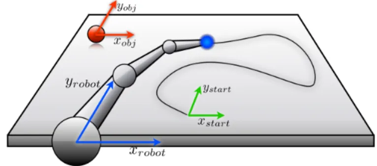
The world consists of a 2D simulated robot hand and one object (we assume we have a 2D multi-link arm with a pre-cise inverse kinematics model which allows to directly work in the operational space of the hand). During demonstrations a demonstrator takes the simulated hand of the robot and moves it (using the mouse), hence we set ourselves in the kinesthetics demonstration framework, as in [1]. The state space of the system is 8 dimensional and includes the 2-D position of the robot hand in 3 different frames of reference, as can be seen if figure 3. One coordinate system is centered on the starting position (xs,ys), one is centered on the robot
(xr,yr) and one is centered on the object (xo,yo). We write
the position of the hand in these three coordinate systems as
(Hxs,Hys), (Hxr,Hyr) and (Hxo,Hyo). We write the position of
the object in the coordinate system of the robot as (Oxr,Oyr).
From this set of 8 dimensions we define 3 different subsets: • Framing 1: Hxs, Hys, Oxr and Oyr
• Framing 2: Hxr, Hyr, Oxr and Oyr
• Framing 3: Hxo, Hyo, Oxr and Oyr
Finally, the action space of the robot is 2 dimensional and consists in setting the speed vector of its hand. The speed is the same in all the 3 coordinate systems since they all have the same orientation.
Fig. 3. Here we see the 3 coordinate systems of the experiment. In the text we will write xstartas xs, xrobotas xretc, for short. The 8 dimensional
state space consists of the hand position in all 3 coordinate systems plus the position of the object in the coordinate system of the robot.
There are 4 different tasks with 5 demonstrations for each task, and the element of context which characterizes each task is the location of the object. The first task is ”move hand to object”, which is demonstrated/should be reproduced when the object is in the upper left corner (but with varying precise positions). The second task is ”draw an S from your starting position”, which is associated to a position of the object in the upper right corner (again at varying precise positions). The third task is ”encircle the object”, associated to the object in the lower left corner, and the fourth task is ”move your hand in a big cyclic rounded edges squared shape relative to you” and is associated to the object in the lower right corner. The relevant dimensions (not told to the robot) are hand relative to object in the first and third task, hand relative to starting position in the second task and hand relative to robot in the fourth task.
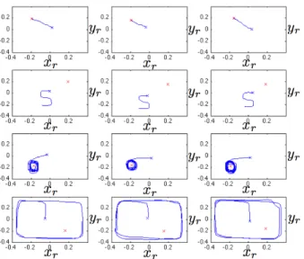
The demonstrations are made using a mouse movement capturing function in Matlab. The starting position and object position is assigned randomly within a square of the figure (the starting position in a square centered on the middle and the object is placed somewhere in a square centered in a corner) and plotted in a figure. The demonstrator then clicks a mouse button once and drags the mouse performing the demonstration and clicks again when the demonstration is completed. The positions of the mouse is registered and used to calculate the speed and the relative positions. We can see the tasks demonstrated in figure 4. We can see 5 demonstrations of each of the 4 different tasks in figure 5. A. Reproduction while introducing additional tasks
To make sure that our algorithm can handle new tasks being added we show reproductions of the 4 different tasks in
Fig. 4. This figure shows 3 individual demonstrations of the 4 different tasks. The top task will be referred to as task 1 in the text, the second highest as task 2, etc. The red cross is the position of the object and the blue cross is the starting position of the hand.
figure 6, to the left we see the tasks reproduced with only data of demonstrations of that particular task. The second column shows reproductions after the demonstrations of one more task has been added, the third column shows reproductions after demonstrations of 2 additional tasks have been added and the 4th column furthest to the right show reproductions when all the demonstrations of all the tasks have been made available to the agent. We can see no general trend of task degradation as demonstrations of more tasks are added. In the remainder of the paper all reproductions shown are of agents that have been shown demonstrations of all tasks (but again, without categorical information).
B. Reproductions outside normal starting positions
We test the reproduction ability when starting positions are chosen outside the area where the demonstrations started from, and see the results in figures 7 to 10, for tasks 1 to 4 respectively. In all figures the demonstrations are shown in the correct framing of the task to the top left and then the reproductions are shown in the 3 different framings, all with hand-starting position to the top right, hand-robot to the bottom left and hand-object to the bottom right. The full data of all tasks is available to the agent.
C. Do the framings make a difference?
In order to determine if the framings are necessary we compare the performance for motor task 2 with the algorithm presented above with the performance of an algorithm that picks only one set of local point where distance is measured in all available dimensions (other than the way the local points are picked the algorithm is identical). In order to make a better comparison we start all demonstrations at the starting position (0.03,0.03) (relative to the robot). The difficulty of this task is dependent on the starting position so assigning different random starting positions to the two algorithms
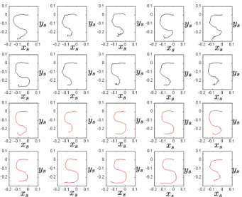
Fig. 5. This figure shows 5 different demonstrations for each of the 4 different tasks. The blue figures to the left shows the demonstrations in the framing of hand position relative to the robot, the red figures in the middle show hand positions relative to the object and the green figures to the right show hand positions relative to the starting position. We can see that the demonstrations are more similar if viewed in the correct framing for that particular task.
Fig. 6. This figure shows that the tasks are successfully reproduced after demonstrated and that adding demonstrations of additional tasks does not destroy performance (one additional task in the second column, 2 in the third and all the other 3 in the fourth).
would just add noise. In figure 11 we see 10 reproductions using the algorithm without framing in the top two rows and 10 reproductions using the proposed algorithm in the bottom two rows. We see that the algorithm presented have some problems but in general outperforms the algorithm not using framings. We also see that it is the second part of the task that is the most problematic for both versions.
D. How many demonstrations are needed?
In order to find the relevant dimensions the demonstrations has to be similar in the relevant dimensions and different in the irrelevant dimensions. We can see in figure 12 that
Fig. 7. This figure shows demonstrations of task 1 (move hand to object) in the framing relative to the object to the top right and the reproductions in the framing relative to the starting position to the top right, where we can see that the reproductions look very different due to the different starting positions. To the bottom left we see that despite starting at different locations the hand moves to the top left corner (the object is always somewhere in the top left corner). Finally we can see to the bottom right the reproductions in the correct hand-object framing. There are some odd behavior at times but in general the task is achieved even when starting outside the area that the demonstrations started within.
indeed the important aspect of the demonstrations is if they contain enough information for the robot to determine what the relevant dimensions are. This means that the amount of demonstration needed is such that for each incorrect framing f there is at least one pair of demonstrations which are different from each other when viewed in f. This requirement can be alleviated if the agent is given the correct framing or have well calibrated prior probabilities from learning other tasks. If a human is demonstrated a task where the demonstrator moves his hand around a coffee mug, the subject is unlikely to assume that the task consists of moving the hand in a circle 50 centimeters to the right of the computer (if the robot is to be able to learn this autonomously it will need to extract relevant rules from previously learned tasks; unless this is done the coffee mug will have to be moved and another demonstration made so that the agent sees that the demonstrations look the same if focusing on the relative position of the hand and the coffee mug but not if focusing on the relative positions of the hand and the computer)
IV. CONCLUSIONS AND FUTURE WORK
We have shown that the ILO-GMR approach allows a robot to learn to reproduce several different context-dependant tasks at the same time and incrementally with-out the need to change any parameters as new tasks are added, and without categorical information associated to each demonstration. Future work will concentrate on evaluating this approach in experiments with real robots and with more varied motor tasks and sensorimotor contexts. Also, we will investigate, among other things, how unsupervised tech-niques for clustering motor tasks may (or may not) improve
Fig. 8. This figure shows demonstrations (top left) and reproductions
of task 2 (draw an S shape). We can see that, as we should expect, the reproductions look similar to the demonstrations in the framing of hand relative to starting position (top right). A few of the reproductions does not completely replicate the task in the last turn but overall the reproductions are similar to the demonstrations
Fig. 9. This figure shows the demonstrations and reproductions of task 3 (move hand in circle around object).
Fig. 10. This figure shows demonstrations (top left) and reproductions of task 4 (make a big cyclic square movement). The task is largely reproduced as demonstrated.
Fig. 11. This figure shows at the top two rows in black 10 reproductions made while picking only one set of local points using distance in the full state space. The bottom two rows shows the results using framings. we can see that on average the S shape is better in the bottom two rows, especially the later half of the movement (the second ”turn”).
Fig. 12. This figure shows at the top row demonstrations nr 1 and 5 in first framing 2 (blue), then framing 3 (red), then framing 1 (green) and finally 5 reproduction attempts in framing 1 (the correct one for task 2) of an agent able to see all demonstrations of the other tasks and demonstrations 1 and 5 of task 2. The bottom row is exactly the same but with demonstrations 3 and 5 instead. The demonstrations at the top look the same in two different framings and as a result the agent will not know what framing is the correct one and the reproduction attempts suffer as a result. The demonstrations at the bottom are different in the two incorrect framings but similar in the correct one giving the agent a chance to find the correct framing and as a result these reproductions (bottom right) is superior to the other reproductions (top right).
the performances of the system, as well as how to integrate an attention system to some degree dependent on what was attended previously, either from a cognitive modeling point of view (more realistic) or from an engineering point of view (guaranteeing smoothness and stability).
REFERENCES
[1] S. Calinon and F. Guenter and A. Billard, On Learning, Representing and Generalizing a Task in a Humanoid Robot, IEEE Transactions on Systems, Man and Cybernetics, Part B , vol. 37, 2007, pp 286-298. [2] Aude Billard, Sylvain Calinon, Ruediger Dillmann, Stefan Schaal,
Robot Programming by Demonstration, Springer Handbook of Robotics., 2008, pp 1371-1394.
[3] Calinon, S., Evrard, P., Gribovskaya, E., Billard, A. and Kheddar, A., Learning collaborative manipulation tasks by demonstration using a haptic interface, Proc. Intl Conf. on Advanced Robotics (ICAR)., 2009. [4] Calinon, S., D’halluin, F., Caldwell, D.G. and Billard, A. Handling of multiple constraints and motion alternatives in a robot programming by demonstration framework. In Proceedings of the IEEE-RAS Inter-national Conference on Humanoid Robots (Humanoids), Paris, France, 2009.
[5] M.N. Nicolescu and M.J. Mataric, Natural methods for robot task learning: Instructive demonstrations, generalization and practice, Pro-ceedings of the International Joint Conference on Autonomous Agents and Multiagent Systems (AAMAS)., 2003, pp 241-248.
[6] M. Pardowitz, R. Zoellner, S. Knoop, and R. Dillmann, Incremental learning of tasks from user demonstrations, past experiences and vocal comments, IEEE Transactions on Systems, Man and Cybernetics, Part B. Special issue on robot learning by observation, demonstration and imitation, 2007, pp 322-332.
[7] S. Ekvall and D. Kragic. Learning task models from multiple human demonstrations, Title, Proceedings of the IEEE International Sympo-sium on Robot and Human Interactive Communication (RO-MAN)., 2006, pp 358-363.
[8] A. Alissandrakis, C.L. Nehaniv, and K. Dautenhahn, Correspondence mapping induced state and action metrics for robotic imitation, IEEE Transactions on Systems, Man and Cybernetics, Part B. Special issue on robot learning by observation, demonstration and imitation., vol. 4, 2007, pp 299-307.
[9] Nehaniv, C., and Dautenhahn, K., Of hummingbirds and helicopters: An algebraic framework for interdisciplinary studies of imitation and its applications, Interdisciplinary approaches to robot learning.,World Scientific Press, vol. 24, 2000, pp 136-161.
[10] Nehaniv, C., and Dautenhahn, K., The correspondence problem, Imi-tation in animals and artifacts., MIT Press, 2002, pp 41-61. [11] N. Delson and H. West., Robot programming by human demonstration:
Adaptation and inconsistency in constrained motion., Proceedings of the IEEE International Conference on Robotics and Automation (ICRA)., 1996, pp 30-36.
[12] Ude, A, Trajectory generation from noisy positions of object features for teaching robot paths, Robotics and Autonomous Systems., 1993, pp 113-127.
[13] Ito, M., Noda, K., Hoshino, Y., and Tani, J, Dynamic and interactive generation of object handling behaviors by a small humanoid robot using a dynamic neural network model, Neural Networks. , 19 (3), 2006, pp 323-337.
[14] Calinon, S. and Billard, A, Incremental Learning of Gestures by Imitation in a Humanoid Robot, Proceedings of the ACM/IEEE International Conference on Human-Robot Interaction (HRI),., 2007, pp255-262.
[15] Calinon, S Robot Programming by Demonstration: A Probabilistic Approach.,EPFL/CRC Press , 2009.
[16] A. Dempster and N. Laird and D. Rubin, Maximum likelihood from incomplete data via the EM algorithm, Journal of the Royal Statistical Society. B, 39(1):, 1977, pp 1-38.
[17] Yeung, D.Y. and Zhang, Y., Learning inverse dynamics by Gaus-sian process regression under the multi-task learning framework. In The Path to Autonomous Robots, G.S. Sukhatme (ed.), pp.131-142, Springer, 2009.
[18] Vijayakumar, S. and Schaal, S., LWPR : An O(n) Algorithm for Incre-mental Real Time Learning in High Dimensional Space, Proc. of Sev-enteenth International Conference on Machine Learning (ICML2000) Stanford, California, pp.1079-1086, 2000.
[19] Nguyen-Tuong, D. and J. Peters: Local Gaussian Processes Regression for Real-time Model-based Robot Control. Proceedings of the 2008 IEEE/RSJ International Conference on Intelligent Robots and Systems (IROS 2008), 380-385, IEEE Service Center, Piscataway, NJ, USA, 2008.
[20] Chang, C.C. and Lin, C.J., LIBSVM: a library for support vector machines, http://www.csie.ntu.edu.tw/ cjlin/libsvm, 2001.
[21] Angeli, A., Filliat, D., Doncieux, S., Meyer, J-A., A Fast and In-cremental Method for Loop-Closure Detection Using Bags of Visual Words. IEEE Transactions On Robotics, Special Issue on Visual SLAM. 2008.
[22] Zoubin Ghahramani and Michael I. Jordan, Supervised learning from incomplete data via an EM approach, Advances in Neural Information Processing Systems. vol. 6, 1994, pp 120-127.