HAL Id: hal-02191390
https://hal-lara.archives-ouvertes.fr/hal-02191390
Submitted on 23 Jul 2019
HAL is a multi-disciplinary open access
archive for the deposit and dissemination of sci-entific research documents, whether they are pub-lished or not. The documents may come from teaching and research institutions in France or abroad, or from public or private research centers.
L’archive ouverte pluridisciplinaire HAL, est destinée au dépôt et à la diffusion de documents scientifiques de niveau recherche, publiés ou non, émanant des établissements d’enseignement et de recherche français ou étrangers, des laboratoires publics ou privés.
(USA) et du DLR (RFA)
P. Olivier
To cite this version:
P. Olivier. Analyse de la qualité image et inter-étalonnage des radars à ouverture synthétique aéro-portés du JPL (USA) et du DLR (RFA). [Rapport de recherche] Note technique - CRPE n° 189, Centre de recherches en physique de l’environnement terrestre et planétaire (CRPE). 1990, 58 p., illustrations, tableaux, graphiques. �hal-02191390�
Centre Paris B Département TOAE
CENTRE DE RECHERCHES EN PHYSIQUE DE L'ENVIRONNEMENT TERRESTRE ET PLANETAIRE
NOTE TECHNIQUE CRPE/189
ANALYSE DE LA QUALITE IMAGE ET
INTER-ETALONNAGE
DES RADARS
A OUVERTURE
SYNTHETIQUE
AEROPORTES
DU JPL (USA) ET DU DLR (RFA)
par
P. OLIVIER RPE/OBT
38-40 rue du Général Leclerc 92131 ISSY-LES-MOULINEAUX
Le Directeur
^G.-SDMMERIA
Le Directeur Adjoint
MM. FENEYROL Directeur du CNET PAB/BAG/CMM CAQUar THABARD Directeur Adjoint PAB/SHM/PHZ JUY
du CNET PAB/RPE GENDRIN
COLONNA Adjoint Militaire PAB/RPE/OBT CAUDAL au Directeur du CNET PAB/RPE/OBT DECHAMBRE
MEREUR Directeur PAB/RPE/OBT HAUSER
des Programmes PAB/RPE/OBT TACONET
BLOCH DICET PAB/RPE/OPN LEQUEAU
MME HENAFF DICET PAB/RPE/TTS LANCEUN
MM. PIGNAL PAB
RAMAT PAB CCETT - RENNES
NOBLANC PAB-BAG
ABOUDARHAM PAB-SHM DOCUMENTATION
HOCQUET PAB-STC THEBAULT PAB-STS
SOMMERIA PAB-RPE CNFS
GENDRIN PAB-RPE
BERTHELIER PAB-RPE CNES/OT BAUDOIN
BIC PAB-RPE
CERISIER PAB-RPE
LAVERGNAT PAB-RPE EXTERIEUR
ROBERT PAB-RPE
ROUX PAB-RPE GCTS BECKER
VIDAL-MADJAR PAB-RPE DMN/EERM LornERE
MME HAUSER PAB-RPE MARTIN
CNRS
MM. BERROIR TOAE CHARPENTIER SPI MME SAHAL TOAE MM. COUTURIER INSU MME LEFEVRE DR M. DUVAL DR CNES MMES AMMAR DEBOUZY MM. BAUDOIN FELLOUS HERNANDEZ (Toulouse) Bibliothèques CNET-SDI (3) CNET-EDB CNET-RPE (Issy) (5) CNET-RPE (St Maur) (2) Observatoire de Meudon CNRS-SA CNRS-CDST CNRS-LPCE
RESUME
Ce document constitue le compte-rendu technique de la mission effectuée
par l'auteur, de Février à Juillet 1990, au sein du Jet Propulsion Laboratory (USA). Le travail a consisté en une étude comparative, du point de vue de la qualité image et de l'étalonnage, d'images obtenues, sur le site d'Oberpfaffenhofen (RFA), par deux Radars à Ouverture Synthétique aéroportés aux caractéristiques sensiblement différentes.
L'analyse de la qualité image a permis de mettre en évidence les propriétés spécifiques des deux systèmes, polarimétrie complète du ROS de NASA/JPL et haute résolution multi-vues du ROS du DLR, et d'attester que les objectifs de qualité
respectifs étaient, dans l'ensemble, atteints.
Les images en bande C ont été séparément étalonnées, polarimétriquement
par l'utilisation d'un algorithme développé au JPL et radiométriquement au moyen de coins réflecteurs triédraux disposés à cet effet sur la scène imagée. La '
comparaison effectuée ensuite sur les coefficients de rétro-diffusion de cibles étendues a fourni des résultats encourageants puisque les valeurs obtenues diffèrent de moins de 2 dB.
Enfin, et ceci constitue l'aspect le plus original de ce travail, on a montré qu'un inter-étalonnage effectif était faisable entre les deux séries de données , notamment en ce qui concerne la correction radiométrique en site des images ROS.
REMERCIEMENTS
Le travail décrit dans le présent document a été effectué, au cours d'un
séjour de cinq mois, au Jet Propulsion Laboratory, California Institute of Technology, sur un contrat de la National Aeronautics and Space Administration. Le financement du séjour a été assuré par le Centre National d'Etudes des Télécommunications et par le Centre National des Etudes Spatiales. Que le Dr. D.
Vidal-Madjar, responsable du département Observation de la Terre, soit particulièrement remercié pour avoir pris l'initiative d'une telle collaboration.
L'auteur est reconnaissant envers les Drs. F. Li, J. Curlander et R. Kwok de l'avoir accueilli respectivement dans leur section et groupe, A. Freeman d'avoir fourni le sujet de l'étude et de l'avoir fait progresser par de nombreuses et fructueuses discussions, et tous les membres de l'équipe "étalonnage"
(particulièrement P. Dubois, J. Holt et J. Klein) pour la mise à disposition de tout matériel ou logiciel nécessaire ainsi que leur assistance humaine quasi
journalière. Les équipes respectives des ROS aéroportés de NASA/JPL et du DLR doivent aussi être remerciées pour avoir recueilli et traité les données utilisées dans ce travail.
CONTENTS
1. Introduction
1. Description of the experiment
2.1 The JPL multi-frequency, multi-polarization Aircraft SAR 2.2 The DLR C-Band and X-Band E-SAR
2.3 The DLR, Oberpfaffenhofen, experimental site 3. Image quality analysis
3.1 Radiometric resolution 3.2 Spatial resolution
3.21 AIRSAR C-Band images
3.22 E-SAR C-Band and X-Band images
4. Amplitude calibration of the E-SAR C-Band image 4.1 Model for amplitude calibration
4.2 Actual calibration
4.3 E-SAR calibration for distributed targets
5. Polarimetric calibration of the AIRSAR C-Band images 5.1 Model for polarimetric calibration
5.2 Actual calibration
6. Cross-calibration of E-SAR and AIRSAR images 7. Conclusion
REFERENCES TABLES FIGURES
1. Introduction
In summer 1989, the NASA/JPL DC-8 SAR took part in a séries of calibration
experiments in Europe: three différent sites were imaged in the UK (Feltwell), NL (Flevoland) and FRG (Oberpfaffenhofen), and several sensors (including SAR and SLAR) were in opération. The aims of this campaign were multiple: to check the calibration performance of the JPL Aircraft SAR (named AIRSAR in the
following) over European sites, of quite différent texture compared with those previously used in North America; to compare, from the image quality and calibration points of view, the images provided by the différent sensors; to test various equipment and approaches for ground calibration and to help find candidate sites for future satellite missions such as SIR-C and ERS-1.
A detailed description and some preliminary results of thèse multi-sensor
experiments can be found in [1]. In this document, we will deal only with data gathered from the German site over which both AIRSAR and the German E-SAR, the latter on board a Domier D0228, flew along parallel tracks, on the same day of
August 1989. Having at our disposai tne whole fully polarimetric three frequency (L-, C- and P-Band) data set from the AIRSAR and the C- and X-Band, VV polarized, amplitude images from the E-SAR, the purpose of this work was to conduct a comparative image analysis and calibration of thèse two data sets. The main features of such a study should be: to point out the spécifie characteristics of each data set, considering the very différent radars which were in opération (better
spatial resolution for the E-SAR, quad-polarization mode of the AIRSAR...); and to be able to perform effective cross-calibration, i. e. use one calibrated image to
improve the calibration process of the other one.
Check the image quality of the two data sets, using standard tools like radiometric resolution, impulse response parameters.
Perform separate calibration of each image using a subset of the
deployed devices on the airfield; for polarimetric calibration of the AIRSAR data, some algorithms developed at the JPL will be used.
Compare the calibrated images by checking the target responses in areas away from the one used during the calibration process. Improve the E-SAR calibration process (particularly the range radiometric variation), since the
présent standard product of this System does not include ail the necessary corrections, by means of the AIRSAR image, which is considered to be fairly well calibrated because of the previously conducted calibration experiments, mainly Goldstone in Spring 1988 [2],[3].
Finally, original conclusions should be drawn about the usefulness of such cross-calibration analysis; for it is the first time, as far as we know, that SAR
imagery of the same site is performed by two différent radars, under similar conditions.
But let us first give a brief description of the two radar imaging Systems and of the expérimental site at Oberpfaffenhofen.
2. Description of the experiment
2.1 The JPL multi-frequency, multi-polarization Aircraft SAR
The principal parameters of the NASA/JPL Airbome Imaging Radar [4] are
gathered on Table 1: as an expérimental tool for preparing the future SIR-C mission, this System was designed to be multi-frequency (P-, L- and C-Band), fully polarimetric (i. e. providing complex data in each of the four polarization channels HH, HV, VH, VV). The important characteristics to keep in mind are that
basically the same chirp signal is used, for the three frequencies, and that the transmitted pulse is alternatively switched on H and V polarizations within the same puise répétition interval.
The twelve simultaneously acquired cohérent channels are processed using SAR standard frequency domain compression algorithms, with Hamming
weighting function being applied in range and in azimuth, in order to reduce sidelobes (this point is important to be noted for it will hâve a direct conséquence on the image quality parameters such as spatial resolution and sidelobe levels).
Among the three available standard products, high resolution single look complex image, compressed four-look Stokes matrix format or survey mode image, only the first one was used hère. The high resolution format includes twelve separated files, corresponding to each frequency/polarization channel, containing 750 records of 4096 azimuth pixels; the sampling steps are 6.7 m in slant range and 3.0 m in azimuth.
2.2 The DLR C-Band and X-Band E-SAR
The E-SAR System allows imagery in three frequencies, L-, C- and X-Band, with only VV polarization [5]. Since only C- and X-Band data were obtained over the Oberpfaffenhofen site, we report on Table 1 and 2 the radar parameters related to thèse two frequencies. The important characteristics which differ from the JPL radar are the followings (regarding C-Band) :
The platform flies at rather low altitudes, which implies a larger aperture beamwidth in élévation to illuminate a given swath
The theoretical range spatial resolution is smaller than the AIRSAR one, while both SAR azimuth spatial resolutions are of the same order of magnitude.
The raw data are range compressed on board the aircraft, by means of a Surface Acoustic Wave correlator, and the signal is radiometrically controlled by an AGC/STC unit, placed at the puise compression module input, in order to fit the
System dynamic range. A motion compensation procédure is incorporated, prior to the on-ground azimuth compression, which extracts the desired parameters from the range compressed data [6].
The data products we hâve at our disposai are multi-look (4-look C-Band and 8-look X-Band) amplitude detected images in slant range coordinates.
2.3 The DLR, Oberpfaffenhofen, expérimental site
The DLR site, located near Munich in Germany, is centered on the airport area, where the calibration devices were deployed, and contains various
background areas as grasslands, forests, agricultural fields and suburban areas. As shown on Figure 1, a set of 55 pièces of calibration equipment were installed,
m) and dihedrals (0.7 m and 1.0 m), one C-Band receiver unit and one C-Band Polarimetric Active Radar Calibrator. The dihedrals were oriented at 0° and 45°, with respect to the Une of sight direction, by means of a DLR built, very précise
pointing System in azimuth, élévation and orientation. Most of the trihedrals were deployed as single ones, but some of them were gathered in pairs, separated by about 10 m, in order to test the resolution capabilities of the sensors.
On two consécutive days of August 1989, both radars, mounted on board their respective platforms, flew several parallel flights oriented at 42° (parallel to the runway direction) and 132° (orthogonal to the runway) with respect to North, with various incidence angles for the AIRSAR radar (about 20°, 35° and 50° over the airfield main runway).
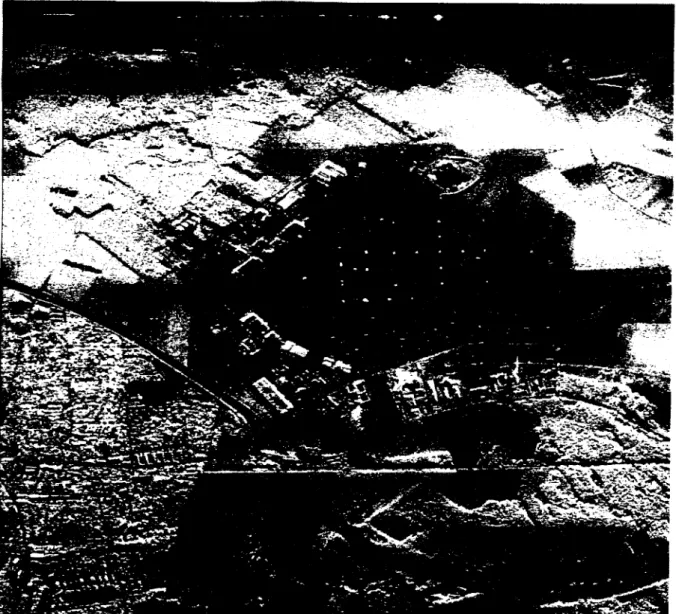
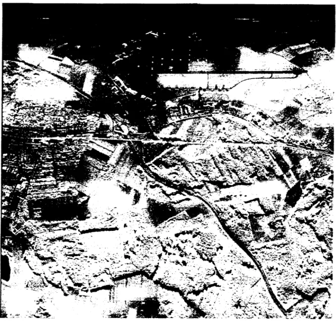
In Figures 2, 3 and 4 are respectively displayed the CVV AIRSAR, CVV and XVV E-SAR images of the test site; ail of them are amplitude detected. The E-SAR
images are not radiometrically corrected; they are direct outputs from the SAR processor. Although we could perform the range radiometric correction, by means of vertical antenna pattern data and incidence angle knowledge, we
preferred to keep thèse raw images, in order to conduct the cross-calibration analysis with the AIRSAR images. On each image, we can clearly see the airfield area with the corner reflector array; the calibration devices which are deployed near the buildings, below the runway, are not so clearly visible on thèse prints, with the exception of the PARC on C-Band pictures, but are more détectable on the
imaging device screen. Scales and aspects of thèse three images are variable to each other because of the différent values taken by the resolution and the pixel
spacing parameters. Table 2 summarizes the image parameters, from the three data sets we will deal with in the following sections, i. e. C-Band quad-polarization AIRSAR, C-Band and X-Band VV polarized E-SAR, ail along the 42° direction flight path.
3. Image quality analysis
To assess the quality of one given SAR image, we usually deal with two main
concepts: the radiometric resolution, which is a measurement of the ability of distinguishing two uniform areas of différent backscattering coefficients, and spatial resolution, which is a measurement of the ability to separate two distinct point target scatterers. Image quality assessment is a very important step in SAR image study because the aim of a SAR is to provide ground reflectivity images with a much better spatial resolution (in azimuth) than a classical radar; so, it is
obviously necessary to check to what extent this goal has been achieved. Moreover, for calibration purposes, with the aim of providing relationships between measured pixel intensities and ground reflectivity parameters, the radiometric resolution is a useful tool to estimate the accuracy of the obtained calibration results.
As such analysis is to be performed within each image and deals mainly with magnitude pixel responses, ail the polarimetric quality checks, which can be made on the AIRSAR data set, will be treated in section 5, as part of the
polarimetric calibration process.
3.1 Radiometric resolution
On SAR images, the response of uniform (also called distributed) targets is disturbed by the well known speckle noise [7], due to the cohérent addition of numerous and independent target responses within a same resolution cell. The
power of this multiplicative noise directly affects the separability of two différent areas, as it widens each probability density function of the pixel intensities; so a standard parameter to quantify the radiometric resolution is provided by the O / \l ratio, where Il and a are the mean and standard déviation of the pixel intensity
distribution over selected uniform areas. (J and Il represent respectively the
multiplicative noise and desired signal powers, so this radiometric resolution parameter can be seen, too, as a signal to speckle noise ratio.
A common way of expressing the radiometric resolution coefficient allows a direct interprétation in dB:
Y = 10 log ( 1 + a/n ) ( 1 )
where O and Il are computed from the power (not amplitude) pixel distribution [8].
Assuming the elementary scatterer responses, within one cell, are complex, independent random variables with the same probability distribution, it can be shown that the power of the resulting signal is exponentially distributed while its phase is uniformly distributed over [0; 2k]. So the radiometric resolution coefficient should be 1 (3.01 in dB) when estimated from power detected single- look uniform areas.
Considering multi-look images, which resuit from the superposition of N independent power detected partial images, the mean and standard déviation of the pixel intensity probability density are respectively multiplied by N and V N , so that the radiometric resolution coefficient becomes:
YN = 101og(l+
;j=) (2)
Thus, in order to assess the image radiometric quality, we selected a set of ten uniform areas (by visual inspection) in each of the three images (only CVV was considered in the AIRSAR case) and then computed the associated y
coefficient. The average results are reported on Table 3, as well as the expected values, from (2), knowing that the AIRSAR data are 1-look (since they are, actually, complex images) and the E-SAR data are respectively 4 (C-Band) and 8 (X- Band) look images.
Measured and expected values for the AIRSAR CVV image are in good
agreement, but, conceming the E-SAR, measured values are higher than expected (the différence is more important for the X-Band image). This discrepancy can be explained by the fact that the four, or eight, looks are not perfectly independent to each other, hence a less efficient speckle noise réduction: during the multi- look processing, the selected Doppler sub-bands, instead of being completely
disjoined, exhibited a certain amount (50%) of overlap. However, a 50% bandwidth overlap, inducing respectively 2.5 and 4.5 équivalent number of independent looks, should lead to even higher values of the y coefficient.
3.2 Spatial resolution
Spatial resolution properties of a SAR image are most conveniently studied by means of the whole system impulse response (including the measurement radar equipment and the image synthesis signal processor), i. e. the response
provided by an isolated point target scatterer located on an (almost) perfectly absorbing background. Such point targets are the corner reflector devices deployed on the calibration area; they are preferred to natural targets which are likely to be less adequately located and of poorer "point-like" characteristics.
From the two-dimensional impulse response, the following parameters can be extracted to characterize the image spatial quality:
the spatial resolution itself, defined as the 3 dB (half power) width of the main lobe (in the range and azimuth directions)
the Peak Sidelobe Ratio, measured by the level of the highest sidelobe
relatively to the main lobe level, which is relevant to the possible existence of artifacts in the vicinity of the target
the Integrated Sidelobe Ratio, measured by the total power lying in the sidelobes relatively to the main lobe power, which indicates the power amount which is dispersed outside the target actual location and could corrupt other scatterer responses.
Thèse three sets of parameters are directly measurable from the images,
containing many artificial point-like scatterers; summary tables of their values as well as typical plots of the impulse response will be provided in the following sub-sections.
3.21 AIRSAR C-Band images
On Figure 5 are plotted the impulse response magnitude of the 45° PARC, for the four polarization channels; this is the calibration target for which the sidelobes are the most apparent, since it has the best signal to noise (background) ratio (35 dB for like-polarization and 43 dB for cross-polarization). The four
responses are pretty similar, as they must be, because of the theoretical 45° PARC scattering matrix (see (17d)).
Azimuth cuts of the HH and VH polarization impulse responses are plotted on Figure 6, where we can remark that the first sidelobes are only about 17 dB below the main lobe level, whi~h is not as good a PSLR ratio as it should be
expected from the weighting function applied during the SAR processing. For visual comparison purposes, range cuts of 45° PARC and typical trihedral impulse
improvement on the sidelobe energy (better ISLR) but not on sidelobe maximum peak level.
Considering azimuthal corner reflector impulse responses, some trihedrals exhibit the double peak feature shown on Figure 8-a, associated with a poor
general response behaviour. This tendency was reported previously, during the Goldstone calibration experiment in 1988 [3], and it was thought there was some
problem due to the lack of motion compensation algorithm within the SAR processor, so that the data could be processed with a badly estimated drift angle. Of course, in such cases, the définition of main and side lobes should be taken with caution, and hence the 3 dB widths and sidelobe levels should not be very significant.
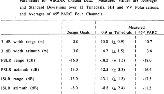
A summary of the impulse response parameters is given in Table 4: the measured values are statistical means and standard déviations among the thirteen 0.9 m trihedrals (taking into account both co-polarization channels) and averages over the 45° PARC four channels. The expected values were estimated during pre-
flight System analysis and simulations; thèse calculations did not take into account the weighting functions which were actually introduced in the processor. So, the measured values are somewhat différent from the predicted ones: greater 3 dB widths and better PSLR (the expected effects of a weighting function). The poor measured azimuth PSLR value from the trihedrals is to be related to the double-
peak feature reported above. Anyway, the trihedral measured values are on the whole fairly close to the ones obtained during the Goldstone experiment [3], at least the mean values since there are some discrepancies among the standard déviations, which means a good long term stability of the AIRSAR performance. The PARC results are better than the trihedral ones as expected from the impulse
3.22 E-SAR C-Band and X-Band images
The same kind of quality checking plots are shown, for the E-SAR System, on Figures 9, C-Band 45° PARC impulse response, 10 and 11, C-Band and X-Band
typical 0.9 m trihedral response. The first thing we can notice, this is particularly clear on the PARC signature, is the discrepancy in the range and azimuth sidelobe
pattems: it is much higher in the range direction. This is, probably, due to the on board range processing of the raw data, by means of an analog SAW correlator, which is a less efficient method than numerical ones. Secondly, the PARC impulse
response is much improved, regarding the sidelobe levels, with respect to the trihedral one; this is particularly true in the azimuth direction. Such an
improvment was not so obvious in the AIRSAR case. This feature is the resuit of the multi-look processing which flattens the sidelobe pattern and makes it reach the background level (see the range and azimuth cuts of Figure 11); so the higher PARC signal to background ratio leads directly to a better PSLR coefficient.
On Table 5 are reported the measured impulse response parameters from the thirteen 0.9 m trihedrals and from the C-Band PARC. The estimated resolutions are pretty close to the predicted ones (see Table 2), except for the X-Band 3 dB width in azimuth, where the 4.0 m expected value maybe is under-estimated
regarding the 8-look process which was applied.
When comparing with C-Band results of Table 4, the différence between the numerical values of the PSLR and ISLR parameters confirm the sidelobe pattern réduction brought by the multi-look processing. This is true as well for the azimuth direction, where both system space resolutions are of the same order of
magnitude, as for the range direction, where E-SAR spatial resolution is much smaller. Only the range ISLR improvement is less important, for the above mentionned reason of analog range processing of the data.
Finally, the main feature of this comparison analysis is the much lower variability of the impulse response parameters over the C-Band trihedral data, as pointed out by the standard déviation low values.
So, one of the most interesting conclusions we can draw from this comparative quality analysis is that the SAR multi-look processing, while primarily designed in order to increase the image radiometric resolution by reducing the speckle noise power, also improves the impulse response quite well. We must note that thèse good spatial resolution properties of the multi-look image
imply that there was no offset problems between the individual images (or they were well corrected), prior to their superposition.
4. Amplitude calibration of the E-SAR C-Band image
4.1 Model for amplitude calibration
The assumptions we will make, in order to establish the relationship between the pixel intensities of one SAR image and the terrain backscattering
parameters, are the followings: first, point target, clutter area and noise responses are three différent processes which are statistically independent to each other, so that the received signais add in power to form the measured pixel
intensity; secondly, the best estimate of point target cross-section is provided by the integrated pixel power over a sufficiently large area containing most of the scatterer impulse response energy, as was recommanded by [9].
Thus, the radar équation, giving the measured integrated power Pr over an area A surrounding one given point target scatterer, can be formulated as [10]:
(47t)3R4 where
- a ( = Ot + A a" ) is the total cross-section (clutter+target) of the area A. -
Pt is the transmitted power
- G is the antenna gain, in the target direction - 1 is the radar wavelength
- R is the slant range
H is the SAR gain, including the processing gain - Pn is the noise power, integrated over A.
Pr = CK(R)Ot + C K(R) crO A + Pn (4)
with C =
Pt X2 is a constant term and K(R) = H G2 is the range (or
incidence angle) dépendent factor.
Let us apply the previous formula to three différent areas within a local
part of the image (where the noise and clutter properties are constant): . A3 where there is only noise:
P3 = Pn = PnO A3 (5)
where PnO is the noise power density
. A2 where there is clutter and noise:
P2 = ( C K(R) crÛ + PnO ) A2 (6) . Ai where the studied point target scatterer lies, which response is mixed with the noise and clutter area:
Pi = C K(R) at + ( C K(R) a° + PnO ) Ai (7)
From (6) and (7), we can dérive the calibration factor expression, as a function of the measured Pi and P2:
C K(R) = Pl - P2 AlI A2 (8)
crt
and, then, from (5) and (6), we obtain an estimate of the distributed target backscattering coefficient:
° P2 1 A2 - P3 1 A3 0
C K(R) (9)
The R dependence, in the previous relationships, only means that ail the
integrated power calculations should be performed over areas of same slant range;
consequently, the obtained calibration factor should be valuable only over a small slant range interval.
4.2 Actual calibration
The same set of thirteen 0.9 m trihedrals (see Figure 1) was used to perform
amplitude calibration of both E-SAR and AIRSAR images: they constitute the only set of identical corner reflectors in sufficient number to allow reasonable RCS estimation by computation of their average responses; moreover, they lie on a
ground area of limited size, thus avoiding the effects of the range radiometric variation shown by the E-SAR images.
A summary of thèse trihedral responses is given in Figure 12, where the
integrated power, minus background power, is plotted in dB versus the scatterer location in range, Figure 12-a, and in azimuth, 12-b, for both frequency bands. The integrated power minus background power is an estimate of the numerator of
(8), apart from a multiplicative constant (additive in dB) which is the pixel size (1.5 x 1.5 m2 in slant range).
By examination of the C-Band plots, it can be stated that there is no significant variation among the corner reflector responses, neither in range nor in azimuth, except for a fade affecting three trihedrals located within a common
range line. This fade is to be related to a gênerai atténuation which affects several contiguous range lines of the C-Band image, as it can be observed from a thorough examination of this image radiometry. So, this is an artifact, the cause of which is not exactly known (maybe an inaccurately estimated azimuthal
référence function during the SAR processing), and thèse three corner reflectors should be removed for further studies.
Considering the X-Band plots, the corner reflector responses exhibit large fluctuations, with a standard déviation of 1.9 dB, and a general level increase with
range location; thèse variations can be explained by the location of the calibration area, near the image top edge, where the antenna pattern fall-off effect is too much important. So, no reasonable. calibration procédure of this
image could be attempted with such features; thus, in the following of this E-SAR calibration section, we will only deal with the C-Band data set.
Since the ten selected corner reflectors are identical 0.9 m trihedrals and are close enough to each other to produce no range response variation, an estimate Si of the integrated power minus background associated with this kind of
scatterer is provided by the calculated average over thèse targets:
Si = 75.6 dB with s. d. = 0.2 dB
The theoretical radar cross-section of a triangular trihedral of maximum
length a, at frequency f, is [11]:
471 a4 f2 RCStri =
3 c 2 (10)
The E-SAR C-Band frequency is 5.3 GHz and a = 0.9 m, so RCStri = 29.3 dB
and the calibration correction factor for point target cross-section estimation is
4.3 E-SAR calibration for distributed targets
From équation (9), it appears that the calibrated value of the
backscattering coefficient of any given distributed target is provided by the différence between the mean pixel power density and the noise power density, divided by the calibration factor C K(R). Thèse mean power densities should be calculated over large enough areas, in order to greatly reduce the speckle contribution in the uniform area response. As the previously given value of Si is in reality the total pixel power within the intégration area (i. e. the integrated
power divided by the pixel area), the calibration factor to get the backscattering coefficient is
- C K(R) (dB) - Ag (dB) or
- C K(R) (dB) - As (dB) + 10 log (sin 6) (11)
where
Ag and As are respectively the ground and slant pixel size, and 9 is the incidence angle.
In the area where the trihedrals were deployed, 8 = 40° and the pixel sizes
are 1.5 m in slant range and azimuth for C-Band data. So the calibration correction factor for distributed target backscattering coefficient détermination is -51.7 dB.
5. Polarimetric calibration of the AIRSAR C-Band images
5.1 Model for polarimetric calibration
The aim of a fully polarimetric SAR is to provide measurements of the
target scattering matrix:
The
Sij complex élément of S is the target response when one i-polarized wave is transmitted and the measurement is made on the j-polarized receiver; hère i and j represent one of the orthogonal horizontal and vertical polarizations. Since any given polarization state can be written as a linear combination of thèse two former ones, we can dérive, from the S knowledge, the target response
corresponding to arbitrary transmit and receive polarizations [12].
Assuming a linear model to describe the transmitter and receiver perturbations, the observed scattering matrix 0 can be written, as a function of the desired one S:
^ Ohv Ow J y Rvh Rvv Shv SVv J y Thv Tvv Nhv Nvv
where N =
{Njj} is an additive noise matrix and R = [Rij and T = {Tjj} are the receive and transmit matrices:
Tij (resp. Rij) is the transmit (receive) j-channel response to i-polarized incident radiation; in (13), the transposed notation in the receiving matrix only means that the receiver is seen as a transmitter acting in the reverse sensé.
Ignoring the noise matrix N in (13), if we want to retrieve the desired scattering matrix S from the observed 0, we hâve to détermine the T and R perturbation matrices (this is the purpose of polarimetric calibration). The transmitter and receiver matrices can be split into three terms in order to
separate différent effects:
T = (Thh TwJ " Thh [Thv/Thh 1 v ) (0 Tvvo/Thh (14) and _ (Rhh Rvh"|_ f 1 Rvh/Rvv^j (Rhh/RVV 0 \ Rhv Rvv Rhv/Rhh 1 ) ( 0 1
So the observed matrix can be re-written as:.
fRhh/RwOy 1 RhV/Rhh) f 1 Tvh/TwVl 0 \ °"ThhRvVl 0 lJI^Rvh/Rw 1 S Thv/Thh lOT vv/Thh + N (16)
where the following terms hâve been isolated: Rhv/Rvv, Rvh/Rvv, Thv/Thh and
Tvh/Tvv terms produce cross-polarization contamination (so called "cross-talk" terms); Rhh/Rvv and Tvv/Thh are the channel imbalance terms between the two orthogonal polarizations; and Thh- Rvv is the absolute calibration factor.
Several algorithms [13] [14] [15] hâve been developed to provide estimâtes of thèse calibration parameters from a given polarimetric image: generally, they use various combinations of known point targets (Polarimetric Active Radar Calibrators, trihedrals, dihedrals,...), located in the imaged scène, the number and configuration of which depending upon the assumptions made on the backscattering S and system T and R matrices. The calibration technique we hâve
used in the présent study [16] avoids the drawback of needing numerous man- made corner reflectors and is based upon a minimum set of hypothesis: the
backscattering statistics of natural distributed targets within the image are used to remove the cross-talk contamination, only assuming the scatterers are reciprocal (i. e. Svh = Shv) and the like- and cross-polarized channels are uncorrelated, which is theoretically assessed in the case of azimuthally symmetric natural targets [17]; known corner reflectors, as trihedrals, can then be used to eliminate the channel amplitude/phase imbalance and to absolute calibrate the data. The principal steps of this algorithm are given in the following:
cross-talk removal: compute the covariance matrix of S from distributed
targets in the area of interest, assuming some kind of spatial ergodicity; solve équations derived from (16), using both previously mentionned assumptions, in the croos-talk parameter unknowns Rhv/Rvv. Rvh/Rvv, Thv/Thh and Tvh/Tvv; this resolution involves some itérative process in order to estimate the corrélation coefficients of the cross-polarization scattering terms Shv and Sv h
channel imbalance removal: the availability of a trihedral corner reflector in the studied scène allows détermination of the Rhh/Rvv and Tvv/Thh
terms, since the HH and VV responses of a trihedral are known to be identical absolute calibration: knowledge of the trihedral cross-section leads straightforwardly to the absolute calibration factor amplitude 1 Thh- Rvv 1. The best way to estimate the measured cross-section of a point target scatterer, from the data set, was adressed in the previous section dedicated to amplitude calibration.
It is to be noted that the whole algorithm assumes th�t the unknown T and R matrices are constant; so it must be applied only to small areas (in the range
direction) and repeted as many times as necessary, in order to correct an entire image.
5.2 Actual calibration
The algorithm we hâve just described above has been applied to the AIRSAR C-Band data to provide polarimetric calibrated images. The first part of this
algorithm, i. e. the covariance matrix computations and cross-talk parameter estimation, was performed using the first quarter of the images (most left-sided on Figure 2), since it was the one which contained the greatest percentage of uniform areas and which was farthest away from most of the point target scatterers (calibration devices on the airport and urban point-like reflectors). Then the cross-talk removal procédure was applied to the whole image with the
previously estimated parameters. The channel imbalance was removed by means of the average measured response from the thirteen 0.9 m trihedrals:
HH/W mean amplitude = 0.2 dB with s. d. = 0.7 dB HH/VV mean phase = 145.4" with s. d. = 3.8°
Finally, absolute calibration was obtained via the known trihedral RCS in order to get backscattering coefficient (�T°) calibrated data files. From the thirteen 0.9 m trihedrals, the mean measured amplitude response was:
HH = 34.5 dB with s. d. = 0.7 dB VV = 34.3 dB with s. d. = 0.3 dB
So, when comparing with the theoretical RCS of 29.3 dB, and taking into account the pixel size (13.0 dB) to get (YO valued data, we obtained an absolute calibration
correction factor of -18.0 dB, which was applied to the whole data.
Before we analyse the results of the calibration process, it is worth
recalling the scattering matrices of the various target types used in the présent experiment:
Strihedral (0 10) 1 (17a) So°dihedral (0 -1 (17b) S45"dihedral = (0 j 0 (17c) S45°PARC = ( 1 1 ^ J (17d)
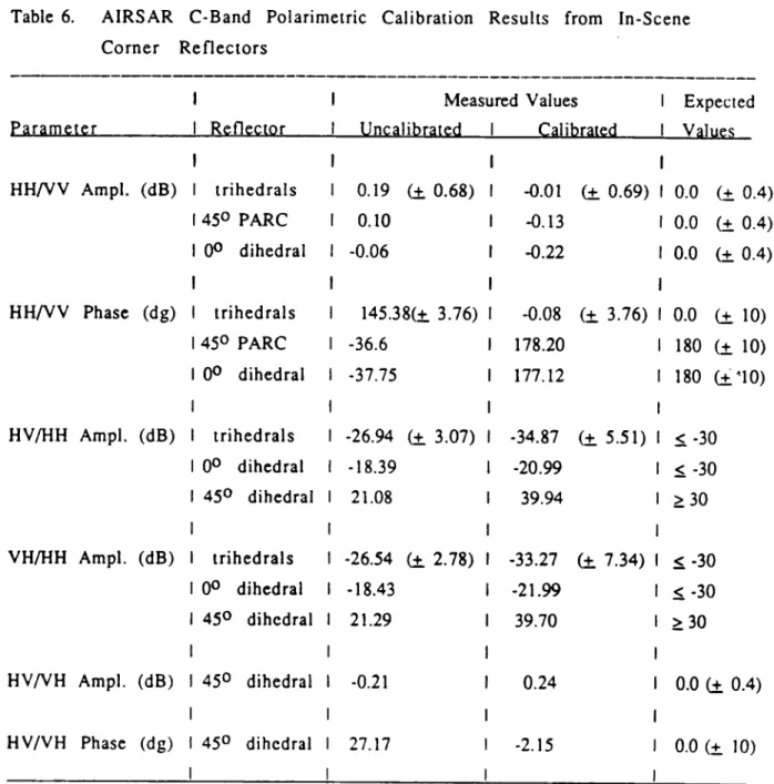
Results of the polarimetric calibration analysis, performed on the uncalibrated C-Band data and on the calibrated ones, are gathered on Table 6. HH/VV ratio is a measurement of the co-polarization channel imbalance, in
amplitude and phase; same kind of information about the cross-polarized channels is provided by the HV/VH ratio, when estimated from rotated devices like 45° dihedrals. Cross-talk contamination estimation is given by the HV/HH and VH/HH amplitude ratios, from trihedrals (unsensitive to orientation), 0° dihedral (line of sight orientation) and 45° dihedral.
From examination of thèse results, we can make the following main comments:
- The uncalibrated data are already well balanced in amplitude, as well for
the co-polarized channels as for the cross-polarized ones; thus, the calibration
process did not improve so much the channel balance, except, obviously, for the trihedrals, of which the mean HH/VV complex ratio was actually used to perform the channel imbalance removal procédure.
- On the contrary, the raw data are not at ail phase calibrated, for the
HH/VV and HV/VH phases are quite différent from the expected ones. The phase balance was achieved on the calibrated data, since the phase values are close to the 0° or 180° expected ones, within the allowable error margin.
- Cross-talk isolation levels are not high enough in the uncalibrated data,
being at least 3 dB below the desired threshold of 30 dB; thèse levels reach acceptable values in trihedral and 45° dihedral calibrated data, while the improvement is very small in the case of the 0° dihedral. For corner reflectors
which are sensitive to orientation, such as the 0° dihedral, maybe that kind of bad cross-talk level can be explained by a non-perfect alignment of the corner reflector respectively to the line of sight direction, as was suggested in [1].
- The increase of the trihedral cross-talk level standard déviations, from
uncalibrated to calibrated data, does not necessarily- mean that the results are less relillable in the latter case; it can be explained by the fact that, with reduced
cross-polarization contamination, the cross-polarized channel responses sometimes can be about or under the background level, thus giving rise to more variable numerical results. Anyway, the essential resuit is preserved, that is to
say thèse responses lie under the desired cross-talk level.
To conclude this section, and to sum up the previous developments, we can assess the polarimetric calibration of the C-Band AIRSAR data has been achieved
6. Cross-calibration of E-SAR and AIRSAR images
Having performed absolute calibration of the two sensor C-Band images of the same site, by means of one set of identical trihedrals, we would like to compare the calibrated responses associated with other targets. As the ultimate goal of
calibrating a SAR image is to provide physical values of the terrain backscattering coefficient, we will focus our attention on the distributed target responses provided by both images. Although the AIRSAR data set is fully polarimetrically calibrated, we will consider, in the following, only the VV- polarized magnitude image.
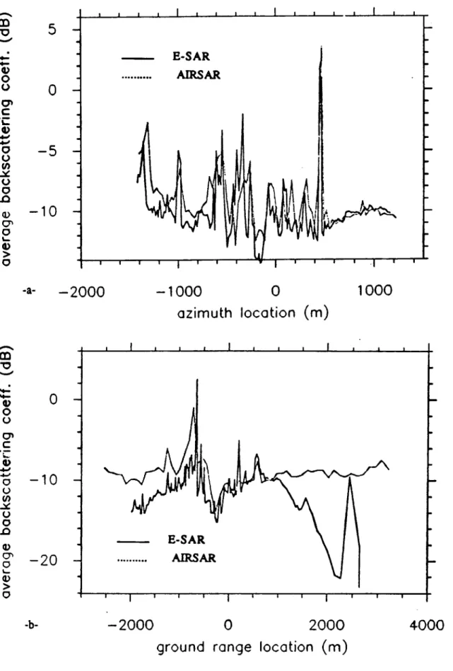
To compare the calibrated data of both radars, the first chosen approach is a global one: the mean pixel power, computed over several lines, is taken as an estimate of the average terrain backscattering coefficient; then, this mean pixel
power is displayed as a function of the other direction, for relative calibration analysis purpose. Of course, the accuracy of such an estimate will be greatly degraded in areas where there are numerous point target scatterers, giving rise to spiky features on the curves. There is no problem when averaging whole azimuth lines, since there is no noticeable distorsion of the pixel magnitude in this direction (except for a few range lines in the C-Band E-SAR image). However, when averaging range lines, we hâve to sélect previously a restricted interval around the main trihedral set (about 2 km wide), because of the E-SAR image
global range variation.
Thèse average backscattering coefficient curves are plotted on Figure 13, azimuth variation of range averaged power on 13-a and range variation of azimuth averaged power on 13-b. For easier comparison between the two data sets, on Figure 13-b the mean power is plotted versus ground position, referred to a common origin (one of the 0.9 m trihedrals). The selected intervais are identical
for both images, in each direction, and the average pixel power is computed over ten consécutive lines. The E-SAR curves exhibit more pronounced high
frequency fluctuations, because of the smaller sampling steps, and resolutions, of this system; we can observe, too, on Figure 13-b, that the sampling steps are
varying along the curves, due to the slant range to ground range conversion.
On Figure 13-a, the AIRSAR and E-SAR curves are very close to each other; even many spiky features are very similar, despite their point-like scatterer
origin. Particularly remarkable is the curve fit at the right-end part of the plot where the areas are more likely to be uniform; hère the curve différence absolute value is always less than 1 dB.
From the E-SAR plot on Figure 13-b, we can easily notice the following features: the global power variation with range is due to the lack of post-
processor range correction (propagation loss, vertical antenna pattern); and the strong peak at the near range end is the nadir return, since the selected range window, in the SAR processor, included distances smaller than the minimal physical one (i. e. the aircraft altitude). But the most interesting resuit is the fact that both curves are pretty similar, in an absolute sensé as well as in a relative
one, over a ground range interval of more than 1 km length around the origin.
The AIRSAR image is well relatively calibrated (it is a confirmation) since the associated curve on Figure 13-b shows no noticeable global range variation. So this curve could be used as a référence in order to perform relative calibration of the E-SAR image across the range swath. But this is rot a simple problem because the two curves do not hâve neither the same sampling frequency nor the same intrinsic resolution, so the calculation of the two function différence should not be so straightforward as it could appear at first sight. In the following, a
compare with a standard theoretical range correction procédure. To do the latter, we first need to know the incidence angle variations with range, which will help, too, explain some discrepancies among the backscattering coefficient values provided by the two sensors. So, on Figure 14, curves of incidence angle versus ground range location are displayed for the two sensors. On the whole, incidence angles are quite différent, particularly for near range areas; but, for the calibration area we are mainly interested in, around the origin, the différence is
only about 5" (about 45° for AIRSAR and 40° for E-SAR), which should not lead to significant différences of the backscattering coefficient [18], if we assume the airport area to be mainly composed of grasslands.
On Figure 15 is plotted, as the solid curve, the empirical correction factor
computed as the différence (in dB) between AIRSAR and E-SAR mean backscattering coefficients, versus ground range; the E-SAR function has been previously smoothed to fit the same sampling step as the AIRSAR one. Only the slow variations of this curve are to be considered, since the sharp and quick fluctuations we can observe are due to unavoidable ground range
misregistrations between the two initial functions. The dashed curve represents the theoretical calibration function, taking into. account ail the range (or incidence angle) effects: vertical antenna pattern, propagation loss and incidence angle correction for backscattering coefficient calculation. From
équation (11) and the expression (4b) of the K(R) factor, we can dérive the formula giving, in power, the calibration correction factor relative to the
backscattering level at the ground origin:
sin (Qo) R(l H(R) G(R)2
The processor gain H(R) is proportional to the squared slant range, as in most standard SAR processors. Thus, the previous expression finally becomes:
sin (eO) RO G(R)2 CAL "
G(RO)2 sin (6) R2
(19)
as it is plotted on Figure 15. The theoretical curve seems actually to be a good fit of the empirical one, at least in an area of more than 2 km length around the origin. Of course, both functions are zero-valued at the ground origin, by the way they are built.
The good fit between thèse two curves indicates that the E-SAR image could hâve been range corrected only by means of an extemal image of the same site, from a sensor with rather différent characteristics. As it is the first time two sensor images are radiometrically compared this way, this is a very encouraging
rosult, ail the more because of the rather preliminary state of the présent cross- calibration study. In case of developing such kind of cross-calibration method, we should be able to define a more elaborate and cautious strategy, by solving the
following problems: how to deal with différent sensor sampling steps and resolutions? how to filter the spiky features due to point target reflectors? what is the best way to modelise the relative calibration function?... But this should be the
subject of future works.
The second way of comparing the AIRSAR and E-SAR calibrated images is more natural and more précise, if performed cautiously!, than the previous one; but it is not much emphasized hère because it nécessitâtes many tideous human
opérations on the displayed images and thus cannot be developed in a systematic manner for further automatic analysis. Some uniform areas are visually selected
on each image, then the corresponding calibrated backscattering coefficient are evaluated, according to (9).
On Table 7 are gathered the comparative results of ten scènes of various terrain types: grasslands, fields and forests are commonly studied végétation terrains; the airport runway and one urban area are added only for comparisons, as respectively représentative of flat target and non-uniform distributed target extrême cases. For sake of completeness, HH channel results are provided from AIRSAR data. Also are given both System incidence angles and radiometric resolution coefficients (standard déviation to mean value ratio of the pixel power
distribution) in order to check the area uniformity and to give some informations about scène texture, as seen by the two sensors.
The given backscattering coefficient values, in the E-SAR case, are corrected in range by the theoretical calibration function examined above. The obtained results are rather good, since the VV 00 différence often lies about or
within 1 dB and is never greater than 2.2 dB; but they are very much variable, in an uninterpretable way: there is no clear corrélation of the resuit quality neither with the terrain type nor with the incidence angle différence. Obviously, the urban area resuit is not good since it is not a uniform target (see the great values taken by the CT/JJ. coefficient). Another and more interesting discrepancies are
exhibited by forest areas, as well from the backscattering coefficients as from the cr/Jl ratios: while the AIRSAR latter values are pretty close to 1, the expected value, the E-SAR ones are quite far away from 0.5 (corresponding to four-look). Maybe this discrepancy can be explained by the différent sensor resolutions, the E-SAR resolution being too small to be able to see forests. as uniform areas; in that case, the scattering mechanism should hâve been created mainly by trunks and branches (which are less numerous in each cell size) rather than by leaves.
7. Conclusion
For the first time, a comparative study of two différent airborne SAR
images of a same site has been thoroughly undertaken: image quality analysis and external, ground target based, calibration hâve been performed, from the NASA/JPL aircraft SAR C-Band and DLR E-SAR C-Band and X-Band data collected over the Oberpfaffenhoffen airport test site in FRG.
On the whole, both System data sets met the image quality requirements associated to their respective characteristics; the only observed discrepancies between theoretical and measured quality parameters could be explained by mis- estimation of some parameters during pre-flight design goal calculations:
weighting functions actually used in the AIRSAR processor were not fully taken into account; and évaluation of the équivalent number of independent looks, in the E-SAR image formation, should be more exactly conducted. The AIRSAR
performance was found to be stable when comparing with the previous Goldstone calibration experiment[3]; even some azimuth impulse response dégradation still remains to be solved, the cause is thought to be the lack of motion compensation
algorithm in the processor. The use of a PARC, compared with trihedrals, for spatial resolution analysis, leads to better impulse response parameter measured values, due to its greater signal to background ratio; particularly, it allowed to point out a discrepancy between the range and azimuth sidelobe patterns, which seemed to be produced by the on board analog range compression scheme used to
process the E-SAR raw data.
The comparative image quality study has shown that the multi-look
processing, more than improving the radiometric resolution, as it is designed for, produced decreased side lobe levels(PSLR and ISLR), and thus improved spatial
resolution, and, what is maybe the most important, more stable and reliable impulse response parameters, over the trihedral set used in the study.
Separate calibration procédures of both system C-Band images hâve been performed, using the same 0.9 m trihedral set. The radiometric calibration process of the E-SAR image has been addressed in détail, particularly focussing on some
aspects which must be treated with care, such as point target RCS estimation taking into account the noise and background response, range dependence of the derived calibration factors, and point target RCS vs clutter 00 formulation. Fully
polarimetric calibration has been performed on AIRSAR C-Band images, by means of clutter backscattering statistics [16]: cross-polarization contamination has been
markedly reduced and phase channel balance has been achieved to a high degree of quality.
Comparison between distributed target backscattering coefficients, evaluated from the previously calibrated C-Band images, gave rather good results, in an absolute sensé, since cr 0 différences always were below 2 dB, but some
variabilty, within each terrain type, was detected. and remained unexplained. A noticeable resuit was that the différent spatial resolutions led to some
discrepancies in the image contrast (radiometric resolution coefficient) on such areas as forests.
Finally, we hâve shown that effective cross-calibration between the différent sensor images was feasible: the radiometric calibration of the E-SAR c- Band image actually could be achieved only by référence to the co-responding AIRSAR image, which was assumed properly calibrated, giving quite similar correction curves as those obtained from more classical methods (i. e. range radiometric correction and absolute calibration by means of known corner
Further works in such direction of calibrating SAR images should include the définition of a cautious strategy mainly in order to deal with sensors of very différent characteristics (spatial resolution, géométrie configuration,...), since
présent and future calibration campaigns may involve various kinds of sensors, such as SARs, SLARs or scatterometers.
REFERENCES
[1] Freeman, A., et al., Preliminary results of the multi-sensor, multi- polarization SAR calibration experiments in Europe 1989, Proc. IGARSS '90, Washington, U. S. A., May 1990.
[2] Freeman, A., Werner, C. and Klein, J. D., Results of the 1988 NASA/JPL airbome SAR calibration campaign, Proc. IGARSS '89, Vancouver, Canada,
July 1989, pp. 249-253.
[3] Freeman, A., Calibration and image quality assessment of the NASA/JPL aircraft SAR during spring 1988, JPL document D-7197, Feb. 1990.
[4] Held, D. N., et al., The NASA/JPL multifrequency, multipolarization airborne SAR System, Proc. IGARSS '88, Edinburgh, Scotland, Sept. 1988, pp. 345-350.
[5] Horn, R., C-Band SAR results obtained by an expérimental airborne SAR sensor, Proc. IGARSS '89, Vancouver, Canada, Juiy 1989, Vol. 4, pp. 2213- 2216.
[6] Moreira, J., A new method of aircraft motion error extraction from radar raw data for real time SAR motion compensation, Proc. IGARSS '89, Vancouver, Canada, July 1989, Vol. 4, pp. 2217-2220.
[7] Madsen, S. N., Speckle theory: modelling, analysi", and applications related to Synthetic Aperture Radar data, Electromagnetics Institute, LD 62, Technical University, Lyngby, Denmark, Nov. 1986.
[8] Brown, L. M. J., et al., SAR data quality assessment and rectification, GEC- Marconi final report, ESA contract n° 6635/86/HGE-I, March 1988.
[9] Gray, A. L., Vachon, P. W., Livingstone, C. E., and Lukowski, T. I., Synthetic aperture radar calibration using référence reflectors, IEEE Trans., GRS-28, n° 3, May 1990, pp.374-383.
[10] Larson, R. W., Jackson, P. L., and Kasischke, E. S., A digital calibration method for synthetic aperture radar Systems, IEEE Trans., GRS-26, n° 6, Nov.
1988, pp. 753-763.
[11] Ruck, G. T., et al., Radar cross-section handbook, Plénum, New-York, 1970, Vol. 2, p.588.
[12] Elachi, C., Spaceborne radar remote sensing: applications and techniques, IEEE Press, 1987.
[13] Sheen, D. R., Freeman, A. and Kasischke, E. S., Phase calibration of polarimetric radar images, IEEE Trans., GRS-27; n° 6, Nov. 1989, pp. 719-731.
[14] Freeman, A., Shen Y. and Werner, C. L., Polarimetric SAR calibration experiment using active radar calibrators, IEEE Trans., GRS-28, n° 2, March 1990, pp. 224-240.
[15] van Zyl, J. J., Calibration of polarimetric radar images using only image parameters and trihedral corner reflector responses, IEEE Trans., GRS-28, n° 3, May 1990, pp. 337-348.
[16] Klein, J. D., Calibration of complex quad-polarization SAR imagery using backscatter statistics, submitted to IEEE AES.
[17] Borgeaud, M., Shin, R. T. and Kong, J. A., Theoretical models for polarimetric radar clutter, J. Electromagnetic Waves and Applications, Vol.
1, n° 1, 67-68, 1987.
[18] Ulaby, F. T., and Craig Dobson, M., Handbook of radar scattering statistics for terrain, Artech House, 1989, p. 179.
Table 2. Parameters of the C-Band AIRSAR, C- and X-Band E-SAR Images Over DLR Site. Resolutions are Theoretical Ones, and Pixel Spacings are Values for the Images Displayed on Figs. 2, 3 and 4.
Table 3. Measured and Expected Radiometric Resolution Coefficients on Uniform Areas from Power Detected AIRSAR and E-SAR Images
Table 4. Spatial Resolution Image Quality: Summary of Impulse Response Parameters for AIRSAR C-Band Data. Measured Values are Averages and Standard Déviations over 13 Trihedrals, HH and VV Polarizations, and Averages of 450 PARC Four Channels
Table 5. Spatial Resolution Image Quality: Summary of Impulse Responsc Parameters for E-SAR C- Band and X-Band Data, Estimated from thirteen 0.9 m trihedrals and from the 45° PARC for C-Band
Table 6. AIRSAR C-Band Polarimetric Calibration Results from In-Scene Corner Reflectors
Figure 13. Azimuth and ground range variations of the average backscattering coefficient, from E-SAR and AIRSAR calibrated CW images
Figure 14. E-SAR and AIRSAR incidence angle variation versus ground range location
Figure 15. E-SAR C-Band relative calibration in the range direction: theoretical (from antenna pattem data) and empirical (from AIRSAR comparison) curves