Matthieu Clertant Nataliya Sokolovska Yann Chevaleyre Blaise Hanczar NutriOmics INSERM Sorbonne University Paris, France NutriOmics INSERM Sorbonne University Paris, France LAMSADE Dauphine University PSL Research University UMR CNRS 7243 Paris, France IBISC
Paris Saclay University Evry University
Evry, France
Abstract
In many prediction tasks such as medical di-agnostics, sequential decisions are crucial to provide optimal individual treatment. Bud-get in real-life applications is always limited, and it can represent any limited resource such as time, money, or side e↵ects of medications. In this contribution, we develop a POMDP-based framework to learn cost-sensitive het-erogeneous cascading systems. We provide both the theoretical support for the intro-duced approach and the intuition behind it. We evaluate our novel method on some stan-dard benchmarks, and we discuss how the learned models can be interpreted by human experts.
1
Introduction
In medical applications, there is an acute need for se-quential rules to acquire patients data, since medical measurements vary tremendously in acquisition cost and in predictive power. There exist numerous exam-ples from clinical practice that illustrate the impor-tance to find a trade o↵ between predictive error of a model and the cost of features used by this model. E.g., the type 2 diabetes remission after a bariatric surgery can be predicted using a set of cheap clinical parameters such as diabetes duration, age, etc., and the prediction is quite accurate for some subjects [1]. However, for a particular group of individuals such a simple model is not accurate enough, and to increase the predictive accuracy, it is advised to measure the
C-Proceedings of the 22nd International Conference on
Ar-tificial Intelligence and Statistics (AISTATS) 2019, Naha, Okinawa, Japan. PMLR: Volume 89. Copyright 2019 by the author(s).
Figure 1: An example of an individualized diagnos-tic protocol: heterogeneous data sources involved in the health status prediction, and their corresponding costs.
peptide what is a rather expensive and invasive proce-dure, and should be avoided for majority of individuals [11]. In this case the clinicians would prefer a cascade classifier which rejects a decision at the first stage if it is not accurate enough, and if there is a hope that a more expensive additional measurement would provide a more accurate patients stratification. Another mo-tivating example is illustrated by Figure 1 that shows that a patient can be stratified using either cheap clini-cal parameters (30 USD), or cliniclini-cal and metabolomics data (what is more expensive and costs 180 USD), or that the expensive metagenomics measurements are needed in addition to the clinical and metabolomics data (with the overall cost more than 1000 USD). Dynamic diagnostic protocols are individually tailored acquisitions of patients data with the aim to provide the most accurate diagnostics for the lowest cost. In contrast with standard approach where all patients follow the same medical protocol, dynamic patients treatment incorporates heterogeneous data, and also the order of medical analyses can vary from one pa-tient to another. Such a dynamic process of papa-tients data acquisition can be called an adaptive strategy. The goal of cascade classifiers under budget constraints
is to classify examples with low cost, and to minimise the number of expensive or time-consuming features (or measurements). Here, under cost we mean the cost paid by a learner during training to acquire relevant information, and at performance time, there is a cost to pay to get relevant information about the current observation. The cost can reflect money or time for data acquisition, or even side e↵ects of a treatment. We adopt a POMDP (Partially Observable Markov Decision Process) framework to model individual op-timal policies under budget constraints. In contrast to much of the existing literature, we propose a method which simultaneously learns classification and rejection models together with the personalized feature selection. Our contribution is multi-fold, and can be summarized as follows:
• We propose a POMDP framework for handling a general dynamic diagnostic protocol setting, and introduce an original methodology to learn indi-vidual adaptive strategies;
• Our method learns cost-sensitive heterogeneous cascading systems;
• We show how a model learned with the proposed method can be interpreted, and how its output can be explained by human experts;
• Numerical experiments on benchmark data show that the proposed method achieves the state-of-the-art performance in terms of accuracy. The qualitative evaluation illustrates that the individ-ualised dynamic strategies allow to stratify ob-servations what can be used in the methods of personalised medicine.
The paper is organised as follows. We discuss the re-lated work in Section 2. We introduce our approach in Section 3. The interpretable deep learning methods are discussed in Section 4. Numerical experiments are shown in Section 5. Concluding remarks and perspec-tives close the paper.
2
Related Work
In this work, we focus on multi-stage sequential reject classifiers that reduce the cost of data acquisition. A number of methods to post-process classifiers in order to reduce their test time complexity were proposed. The largest part of them uses a cascade of classifiers with a reject option. In a cascade, at each stage, a clas-sifier can either classify an input or reject it, and send it to the next classifiers [22, 3]. Most cascade clas-sifiers are usually designed for binary problems, and
aim to reduce computational cost during prediction. The stage cascade classifiers deal with multi-class problems, and they can make a multi-classification de-cision at any stage.
The learning with rejection framework aims to learn simultaneously two functions: a classifier to label an observation and a rejection function [6]. The trade-o↵ between predictive accuracy and rejection rate was studied by [4] where the reject classifiers were consid-ered in the Bayesian setting.
Recent works in the non-Bayesian scenario introduce classifiers with a reject option where the reject region is defined via a distance to the separating hyperplane. A seminal work of [2] provided a theoretical analysis for a discontinuous loss function taking into account the rejection cost.
The problem of classification with reject where a clas-sifier has an option to abstain from taking decision about a label, was discussed in a number of recent publications, and there have been several attempts to integrate a reject option in the state-of-the-art classi-fiers such as support vector machines [9, 7]. A cas-cade system of classifiers with a reject option which minimizes the cost to stratify patients was introduced by [8]. The idea to construct a cascade classifier using trees was exploited by several research teams, e.g., [12] formalised the problem of learning cost-e↵ective mod-els as a Markov decision tree, and employed a vari-ant of the upper confidence bound for trees (UCT). A two-stage algorithm based on random forests and an efficient prunning of all trees simultaneously was proposed by [16].
The most important aspect of cascade classifiers is to learn a function which decides whether to reject an observation or to label it. A problem how to learn a function which is able to identify regions where a low prediction cost model is sufficient compared to a high prediction cost model was considered by [15]. At test time, the method uses the gating function to choose a prediction model.
In [21], the problem of supervised sequential classifi-cation under budget is formulated as a Markov Deci-sion Process (MDP). However, the order of measure-ments or features is fixed and the paper focuses to find reject regions based on known decision bound-aries, which means that the classification models of all stages are learned in advance and are available. The cascade problem is formulated as a simple dynamic programming, and the problem reduced to learning reject regions which are subject specific.
Reinforcement learning is actively explored to pre-scribe optimal treatment where an assessment score
of patients status is used as a reward. A combina-tion of hidden Markov models and deep Q-networks was shown to learn optimal individual heparin dosing for intensive care unit patients [17]. Another combi-nation of modern machine learning methods, namely, of a sparse autoencoder and policy iteration was used in [24] to model personalized optimal glycemic trajec-tories. [18] has shown that optimal quantity of intra-venous medication can be estimated with double deep Q-learning. Tabular Q-learning was proposed in [20] to recommend treatment for schizophrenia patients. A medication strategy for non-small cell lung cancer can be learned by approximating the Q-function using a support vector regression which can incorporate cen-sored data [25].
Recently [23] pointed out that the modern dynamic treatment recommendation systems are learned either by a supervised method, or using reinforcement learn-ing. To combine their benefits, [23] introduced a su-pervised reinforcement approach where recurrent neu-ral networks are used to solve a POMDP.
3
From POMDP to MDP in Cascade
Learning with Reject Option
3.1 Context and PreliminariesIn real-world decision making applications, uncer-tainty comes from two sources: unceruncer-tainty related to the e↵ects of actions and uncertainty about the cur-rent state, i.e., partial observability. The POMDP is a widely used framework to deal with these uncertain-ties. Compared to fully observable MDPs, the uncer-tainty about the current state is a characteristic of POMDPs. In our scenario, the features are gradu-ally observed along the cascade, and a decision can be made from partial observations. The problem can naturally be modeled as a POMDP.
In the problem of diagnostic protocol learning, at each stage of a cascade classifier, the system decides whether to classify an observation, or to continue data acquisition. The process of data acquisition ends when the system is confident enough to return a prediction. What is specific to the task of diagnostic protocol learning, it is that taking an action, i.e., new data acquisition, does not change the state of the patient. Such a POMDP is known as a purely epistemic MDP. A purely epistemic MDP [19] is a much less studied framework, where the actions bring new information without changing the current state.
It is challenging to solve a POMDP, and the problem is often reformulated as a MDP with extended states, e.g., the belief-state MDP or the history-state MDP (see e.g. [10]). For the sake of simplicity, we choose to
build a history-state MDP, where each state consists of the history of all measurements done so far on a patient. Note that such a state does not contain un-observed features or the class of interest. This leads to a fully observable MDP, where standard reinforcement learning algorithms can be applied.
To facilitate the reading, we provide the most impor-tant notations in Table 1. Here, for a purpose of
clar-Table 1: Important notations Notation Description
L Number of classes
K Number of features
t Current depth in the cascade [N ] Set of integers from 1 to N (xi, yi)
i2[N] Observations with classes
xk Feature value k
x[t] Feature values collected prior to t
at Action at step t,
< 0 : feature index, > 0 : class label
a[t] Vector of actions prior to t
c Cost function
V⇧(s) Expected cost from state s
under policy ⇧
Q⇧(s, a) Cost-to-go to a under policy ⇧
Qw(s, a) Approximation of function Q
fw Classifier
rw Rejection/selection model
M[t] Mask corresponding to a[t]
w(.) Weight function of softmax regression
ity, we present our methods with two restrictions. In real life applications, (1) a measurement may be asso-ciated with a group of features as a matrix, sequence, graph or hyper-graph and (2) the cost of a wrong clas-sification depends on the estimated label (e.g false pos-itive or false negative). To simplify the presentation but without any loss of generality, we consider that each measurement is related to one feature only. All the results and observations presented below can be extended directly to any shape of data. We also asso-ciate a cost of 1 to any misclassification. Di↵erentiated weights are hyperparameters of the cascade classifier which can be integrated directly.
3.2 Problem Statement Let (xi, yi)
i2[N] be a training sample from a
distri-bution D : (X, Y ) ⇠ D. We will omit the super-script i in the definition of the supervised learning problem: predicting y from partial or fully observ-able x. The dependent variobserv-able y belongs to the set
of classes [L] ={1, . . . , L} The variable x comes from a large set X consisting of K subspaces of features: x = (xk)k2[K] 2 X with X = X1⇥ . . . ⇥ XK. Each
feature k corresponds to a specific measurement asso-ciated to an acquisition cost k. At each step of the
cascade, the decision process can either choose to ob-serve a new feature or to stop and to return the class ˆ
y. The cost of a wrong classification is 1. The aim is to determine a policy ⇡ of actions minimizing the global cost.
At step t 2 [K], the action at recommended by the
policy belongs to{ K, . . . , L}. In particular, we define two types of actions:
1. at2 { K, . . . , 1}, the policy recommends to
ac-quire feature of index at.
2. at 2 {1, . . . , L}, the policy recommends to stop
acquiring new features, and to provided the pre-dicted label at.
A third (degenerate) category corresponds to the case where the process has been stopped at a previous step: at= 0 if and only if at 1> 0.
3.3 Cascade with Abstention
The state stsummarizes all the observations from step
1 to t : st = (a[t]; x[t]), where a[t] = (ai)i2[t] and
x[t] = (x ai)i2[t] with the convention x ai = ; when
ai > 0. For the sake of compactness in the following
definitions, we set s0=;. The cost function is:
c(st) = 8 < : 1a t6=y with y⇠ Y | st , if at> 0, at , if at< 0, 0 , otherwise. (1) If at = 0, the cost is null (third circumstance). Note
that the cost at step t strongly depends on the last action at which does not appear explicitly in the
pa-rameter as it is included in st. The global cost C and
the cost from step k, noted Ck, are given by:
C(sK) = X t2[K] c(st) and Ct(sK) = X k2[t:K] c(st) , (2)
where [t : K] ={t, . . . , K}. The policy ⇡ is determin-istic and maps the action at with the available data
st 1: at= ⇡(st 1). Let C⇡be the expected cost
asso-ciated to policy ⇡: C⇡ =E
D[C(sK)]. The cost-to-go
from step t, noted V⇡, only depends on policy and
current state st 1:
V⇡(st 1) =ED[Ct(sK)| st 1]. (3)
Q⇡(s
t 1, at) denotes the cost to take a further step in
the direction at, also named the cost-to-go to at:
Q⇡(st 1, at) =ED[Ct(sK)| st 1, at] . (4)
According to the nature of the action, we have:
Q⇡(s t 1, at) = 8 < : PD(at6= Y | st 1) , if at> 0 at+ V ⇡(s t) , if at< 0, 0 , if at= 0.
We emphasize that the order of actions prior to step t does not modify the cost-to-go from step t. The ac-curacy of the model based on st 1is compared to the
acquisition cost of new features and the potential gain in terms of accuracy. Thus, the decision at step t is based on the current state st 1, the “historic state” of
observations to step t, but their order does not play any role. The vector a[t 1]might then be thought as
a vector of indices to identify the feature values x[t 1].
The following properties give some insights in the op-timal solution ⇡⇤:
⇡?= arg min ⇡
C⇡. (5)
Theorem 1. Let ˆy and ˆr be two natural candidates in case of classification and rejection when the distribu-tion D is known: ˆ y = arg max at2[L] PD(at= Y| st 1) , (6) and ˆ r = arg min at2[ K: 1] Q⇡(s t 1, at) . (7)
For all t 2 [K] (or to the end of the cascade), the optimal solution of the MDP system satisfies:
⇡?(st 1) = a?t = 8 > < > : ˆ y , if max at>0P D(at= Y| st 1) > 1 min at<0 Q⇡(s t 1, at) ˆ r , otherwise. (8)
Proof. The trivial case where the cascade has been stopped at a previous step is not considered in this proof. Finding the optimal solution reduces to opti-mize each single stage, and at step t, we have:
a?t = arg min at2[ K:L]\{0} Q⇧(st 1, at) . (9) From there, a?t = arg min at2[ K:L]\{0} [PD(at6= Y | st 1)1{at>0} + Q⇧(st ], at) 1{at<0}] = arg min at2[ K:L]\{0} [{1 PD(at= Y | st 1)}1{at>0} + Q⇧(st 1, at) 1{at<0}] .
Thus, the optimal decision is to stop the feature ac-quisition, and to recommend the class ˆy i↵:
min at2[L] [1 PD(at= Y | st 1)] < min at2[ K: 1] Q⇧(st 1, at) , max at2[L]P D(at= Y | st 1) > 1 min at2[ K: 1] Q⇧(st 1, at) .
If this inequality is not true, the optimal solution would be reject (ˆr) in favor of a new measurement.
4
Deep Models
In this section, we describe how we learn our cascad-ing model. We apply the deep Q-learncascad-ing to estimate it. We are interested in particular in an interpretable model which is able to stratify observations in several groups to promote development of methods of person-alized medicine.
4.1 Deep Q-Learning
DQN (deep Q-network) [14] combines reinforcement learning with deep neural networks. We use the ver-sion with the experience replay that aims to random-ize the data order and to remove correlations in the observation sequence. The complex function Q is ap-proximated by one (or some) neural network(s) with weights w, and the training procedure consists to ad-just the w to the data through the Bellman equation. At iteration j, the Q-learning process is based on the following objective function:
L(wj) =EU (D) h L y; Qwj(s, a) i , (10) with y = c + mina0Qw j(s 0, a0), where U (D) means
that the sample (s, a, c, s0) is drawn uniformly and where L denotes a loss function. In our problem for-mulation, = 1, since we cannot neglect any cost paid in the cascade. The parameters wjare the parameters
of the Q-network at iteration j, and wj are the weights to compute the target at iteration j 1.
The function Q is approximated by two deep neural networks, fw and rw, corresponding to the classifier
(a > 0) and the rejection/selection model (a < 0). Q⇡(s, a)⇡ Qw(s, a) =
⇢
fw(s, a) , if a > 0
rw(s, a) , if a < 0. (11)
The policy estimate is obtained by using the result expressed in equation (8) (see Theorem 1, Section 3). ⇧w(s, a) =
(
yw , if min
a>0fw(s, a) < mina<0rw(s, a)
rw , otherwise,
(12)
with yw= arg min a>0
fw(s, a) and rw= arg min a<0
rw(s, a).
4.2 Interpretable Aspects of the Classifier Although real-valued “black box” classifiers are pow-erful tools in medical diagnostics and prognostics, a model that is able to explain its predictions is of a big interest for clinicians [1]. We are aware that it is possi-ble that there is a price to pay in accuracy for a model which is simple and easily interpretable.
The inputs of both neural networks (fw and rw) are
the current state: st = (a[t]; x[t]). The indices of
fea-tures already observed at current step t, noted a[t],
are encoded as a binary vector mask M[t]of size K: 1
if the feature k has been observed, 0 otherwise. The value of the observed features x[t] might be extracted
from the vector x (all the features) by applying the element-wise product with M[t]. Thus, the state st is
summarized by (M[t], M[t] x). In this vector of size
2⇥ K, an unobserved feature k is associated to a null value for the k th elements of both M[t]and M[t] x.
The classifier fwis a deep neural network, composed of
fully connected layers, and the last layer is based on a softmax regression. The fully connected layers provide the parameters w used in the final regression. They
return a L⇥ K matrix of weights depending only on the mask:
w: (M[t])! w(M[t]) = ( wa(M[t]))a2[L], (13)
where a
w(M[t]) is a vector of size K. The final layer
corresponds to a softmax function taking the vector M[t] x: fw(st, a) = exph a w(M[t]), M[t] xi P a>0 exph a w(M[t]), M[t] xi . (14)
Thus, the values of the observed features, M[t] x,
are used only in the last layer. This together with the small number of features used in most of the circum-stances (see Figures 3 and 5) support the post hoc in-terpretability of the classifier. Moreover, if the human experts focus on feature k observed at time t in the cascade, the product [ a0,k
w (M[t]) wa,k(M[t])]xk is the
weight associated to the features of index k in the log-arithm of the odds of action a against a0. This allows to assess easily the importance and the uncertainty associated to this feature in regard of the decision at time t.
As the interpretability based on the sparsity and the linearity could compromise the accuracy of our method, we choose to associate the classifier with a flexible rejection/selection model, rw which is a
layers. Its ability to identify complex patterns yield-ing to rejection should allow our model to identify the complex cases for which extra information are needed. The input of the rejection/selection model is the vector (M[t], M[t] x) and its output are the approximated
cost-to-go for all the actions which recommend the se-lection of a new features (Qw(a, s))a2{ K,..., 1}.
4.3 Pretraining There are two phases:
1. At first, the classifier is pretrained on all training data. Each observation is associated to a mask drawn randomly (uniform distribution).
2. The rejection/selection model can be pretrained jointly with the classifier by a run of Q-learning. This second phase is optional (details below). In the second phase, the classifier has already been pretrained. We then focus on the rejection/selection model rw. Here, the di↵erence with the training relies
on the input of rw: only the masks are provided and
not the values of features already observed. The input is (M[t], 0K) with 0Ka null vector of size K. An
impor-tant consequence is that the rejection/selection model is not subject-specific anymore. For a certain mask (the labels of features already observed), the evalu-ated cost-to-go to a new feature, rw(s, a) with a < 0,
do not depends of x[t]. The specific choice of
reject-ing or not is then based on the evaluated probability of each label, fw(s, a) with a > 0. Thus, the second
phase of pretraining corresponds to the training of a full cascade classifier model. However, the goal of this model is to identify a unique order for the cascade, optimised for all the subjects.
The model that we propose in this contribution is much more richer, since it is able to identify personal-ized order of features. During the final training phase, the unique order of exploration estimated during the pretraining is used as benchmark to evaluate paths which are now subject specific. The second and op-tional pretraining phase has two e↵ects:
• It decreases the variability of the exploration path.
• It increases the accuracy and as a tradeo↵, the number of features explored.
In the next section, we test the performance of two versions of the introduced interpretable cascade classi-fier with abstention. ICCA stands for our model with only the first phase of pretraining (classifier). When the two phases of pretraining are completed, the model is denoted p-ICCA.
5
Experiments
In this section, we illustrate the performance of the proposed approach. The existing cascading classi-fiers are mostly focused on learning rejection func-tion [21, 16, 15] assuming that the classifiers are avail-able. On the other hand, the literature on classifiers with rejection option [6, 5, 8, 7] studies the rejection function only. Therefore, although quite a rich litera-ture on cascades and on rejections exist, to our knowl-edge, there is no any approach which is directly com-parable to our dynamic feature selection method. After some reflections, we decided to compare our ap-proach to the random forests classifier. The model of random forest with feature selection can be viewed as a static version of a cascade classifier. Indeed, in our approach, the possible costs map with an average num-ber of features observed. To make it comparable, the random forest is based on the same number of features selected by maximal importance criterion. To allow a reliable conversion between the cost and the number of features explored, we assume that all the features have the same cost . The Interpretable Cascacade Classifier with Abstention (ICCA) is expected to have an advan-tage over the random forests classifier in case where it is reasonable to stop the exploration quite early, or, on the contrary, if an extensive individualized feature exploration is necessary for a particular observation. In this section, we discuss our results on two standard benchmarks in details. These sets are downloadable from the UCI Machine Learning repository1[13]:
• Breast Cancer Wisconsin (Prognostic). We dis-pose of about 30 parameters describing charac-teristics of the cell nuclei present in the medical images for 198 patients. All parameters are con-tinuous.
• Mammography. The Mammography set contains 961 observations and 6 variables, and the goal is to predict the outcome of the breast cancer screen-ing, and to avoid unnecessary invasive procedures such as biopsy.
On Figures 2 and 4, we see that both ICCA and the p-ICCA models outperform the random forest classi-fier in terms of accuracy on the two data sets. The number of features shown on the Figures is a mean over the test sample (5-fold cross-validation) estimated by our model. For a fixed value of (the unit cost of a feature), the pretrained version of our model (p-ICCA) has a better accuracy than its standard version (ICCA), but the number of features explored is also
Figure 2: Breast Cancer Wisconsin (Prognostic): Ac-curacy and standard deviation for ICCA (in blue), p-ICCA (in yellow), and the random forest classi-fier (dotted line). The features share the same cost:
2 [10 4, 1/3.10 2].
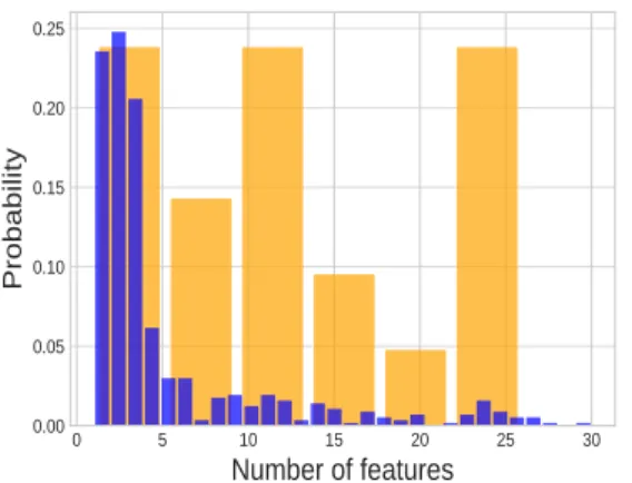
Figure 3: Breast Cancer Wisconsin (Prognostic): his-togram of the number of features explored for ICCA. In blue: all observations (size: 569, mean: 4.8); in or-ange: the misclassified observations (size: 21, mean: 12.3). Overall accuracy: 96,31%.
higher. Thus, for varying in an interval, the accuracy curves for p-ICCA are quite similar to the ones of the ICCA. The histograms on Figures 3 and 5 represent the distribution of the number of features explored be-fore a classification decision by ICCA. The results have been obtained for a fixed parameter cost over the test samples produced by a 5-fold cross-validation. In both cases, the distributions are concentrated around their means. For some patients, the method allows to ex-plore a big number of features. The distributions for the missclassified patients show that, in general, the method allows a longer exploration for patients which are difficult to classify. This is especially true for the Breast Cancer Wisconsin data set: for 75% of the mis-classified subjects, the number of features explored is
Figure 4: Mammography dataset: Accuracy and stan-dard deviation for ICCA (in blue), p-ICCA (in yellow), and the random forest classifier (dotted line). The fea-tures share the same cost: 2 [3.6.10 3, 5.9.10 2].
Figure 5: Mammography dataset: Histogram of the number of features explored for ICCA. In blue: all observations (961, mean: 5,5); in orange: the misclas-sified data (size: 203, mean: 6,7). Overall accuracy: 78,87%.
higher than the average on all data (4.8), 40% of the misclassified individuals are associated to a depth in the cascade higher than 15. This is a sensitive re-sult which shows that our model identifies the difficult cases and tries to collect more information by feature exploration.
The results are less clear for the Mammography task. However, the mean of depth in the cascade for the misclassified data is still significantly above the mean of all observations (Figure 5).
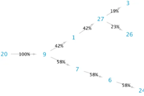
Figure 6 shows obtained exploration paths identified by the p-ICCA (unit cost: = 1/120) on the Breast Cancer data. The nodes are features ids, and the val-ues on the edges reflect the patients percentage in this or that group. It can be observed that patients are
Figure 6: Breast Cancer Wisconsin: The cascade proposed by p-ICCA, exploration path of maximal depth 5 for all patients.
naturally stratified by the algorithm into three clus-ters (or three paths), and three diagnostic protocols can be developed.
The individualized choice of features reveals some nat-ural questions about personalised diagnostic protocols. The weights of the softmax regression of the classifier fw can give some insights in it. If the features 20, 9
and 7 have been observed, the choice of classifying or not can be associated to a strong evidence or a lack of evidence associated to one of the features. This can be explained by studying the di↵erence of weights:
1
20 200, 91 90and 71 70, where 1 and 0 are the
classes (see Eq. (13)). However, the choice of a par-ticular path (e.g., feature 7 instead of 1) is less easy to interpret, since it is related to the interaction between the classifier and the selection/rejection model. We clearly see from the results of the numerical ex-periments, that the proposed method outperforms the random forest on the Breast Cancer and on the Mam-mography data sets. On other tested benchmarks of the UCI repository, such as Bankruptcy, Ionosphere, Haberman’s survival, Mushrooms, and the Glaucoma data, our method achieves a very reasonable perfor-mance, however, it does not outperform the state-of-the-art. We also concluded that for data sets where there is a couple of dominant features (and they are the same for all observations), our method is not really needed.
Implementation details: The neural networks for the rejection/selection model are composed of three fully connected layers. Each layer contains 5 units for the Breast Diagnostic Wisconsin dataset and 4 nodes for the Mammography data set. The activations are the Relu function for the two first layers, and the soft-plus function (x! log(1 + ex)) for the last one. The
loss function is the standard MSE.
The neural networks corresponding to the classifier are composed of two fully connected layers, and the last deterministic layer is the softmax regression (14). The loss function is the cross-entropy. For both neural net-works, we use the Adam optimizer with the learning rate equal to 0.01.
During the Q-learning procedure, we use an ✏-greedy principle starting with 1, with a decay of 0.995 at each episode. The minibatch sample size for the experience replay memory is 32. At each episode, a new cascade associated to one observation is added to the memory. We run 2000 episodes. We also run 2000 episodes for the pretraining (40 epochs are run for the classifier). All above mentioned hyperparameters of the cascade classifier with abstention have been fixed by cross val-idation.
Our implementation in Keras will be made publicly available shortly.
6
Conclusions
The challenge was to develop a principled approach to learn individual diagnostic protocols under limited budget. The proper theoretical support for the pro-posed formulation is provided in Section 3. The result of Theorem 1 provides the theoretical explanations for the optimal decision in terms of classification and re-jection in a MDP system, and a better understanding of the cases where a prediction has to be postponed, and new data have to be acquired.
An important advantage of the proposed method is that its formalization is simple and implementation is straightforward. Our approach does not compromise the usage of the deep Q-networks. In addition, one could easily incorporate the cost values which can be specific for each separate variable or the cost can be defined for groups of variables.
Currently we are investigating novel solutions based on sparse models to make the deep models interpretable. Another avenue of research are various models for clas-sifiers and reject functions. We are also interested to incorporate Monte Carlo Tree Search into the pro-posed cascading framework.
Acknowledgements
The work was supported by the French National Re-search Agency (ANR JCJC DiagnoLearn).
References
[1] J. Aron-Wisnewsky, N. Sokolovska, Y. Liu, et al. The advanced-DiaRem score improves prediction
of diabetes remission 1 year post-Roux-en-Y gas-tric bypass. Diabetologia, 60(10):1892–1902, 2017. [2] Peter L Bartlett and Marten H Wegkamp. Clas-sification with a reject option using a hinge loss. Journal of Machine Learning Research, 9(Aug):1823–1840, 2008.
[3] M. Chen, Z. Xu, K. Weinberger, O. Chapelle, and D. Kedem. Classifier cascade for minimizing fea-ture evaluation cost. In AISTATS, 2012.
[4] C.K. Chow. On optimum recognition error and reject tradeo↵. IEEE Transactions on Informa-tion Theory, 16(1):41–46, 1970.
[5] C. Cortes, G. DeSalvo, and M. Mohri. Learning with abstention. In ALT, 2016.
[6] Corinna Cortes, Giulia DeSalvo, and Mehryar Mohri. Learning with rejection. In Interna-tional Conference on Algorithmic Learning The-ory, pages 67–82. Springer, 2016.
[7] Y. Grandvalet, A. Rakotomamonjy, J. Keshet, and S. Canu. Support vector machines with a reject option. In NIPS, 2009.
[8] B. Hanczar and A. Bar-Hen. Controlling the cost of prediction in using a cascade of reject classi-fiers for personalized medicine. In International Joint Conference on Biomedical Engineering Sys-tems and Technologies, 2016.
[9] B. Hanczar and M. Sebag. Combination of one-class support vector machines for one-classification with reject option. In ECML, 2014.
[10] Hideaki Itoh and Kiyohiko Nakamura. Partially observable Markov decision processes with im-precise parameters. Artificial Intelligence, 171(8-9):453–490, 2007.
[11] AG Jones and AT Hattersley. The clinical utility of c-peptide measurement in the care of patients with diabetes. Diabetic Medicine, 30(7):803–817, 2013.
[12] H. Lakkaraju and C. Rudin. Learning cost-e↵ective and interpretable treatment regimes. In AISTATS, 2017.
[13] M. Lichman. UCI machine learning repository, 2013.
[14] Volodymyr Mnih, Koray Kavukcuoglu, David Sil-ver, Andrei A Rusu, Joel Veness, Marc G Belle-mare, Alex Graves, Martin Riedmiller, Andreas K Fidjeland, Georg Ostrovski, et al. Human-level control through deep reinforcement learning. Na-ture, 518(7540):529, 2015.
[15] F. Nan and V. Saligrama. Adaptive classifiers for prediction under a budget. In NIPS, 2017. [16] F. Nan, J. Wang, and V. Saligrama. Pruning
ran-dom forests for predicting on a budget. In NIPS, 2016.
[17] S. Nemati, M. M. Ghassemi, and G. D. Cli↵ord. Optimal medication dosing from suboptimal clin-ical examples: a deep reinforcement learning ap-proach. Engineering in medicine and biological society, 2016.
[18] A. Raghy, M. Komorowski, I. Ahmed, L. Celi, P. Szolovits, and M. Ghassemi. Deep reinforce-ment learning for sepsis treatreinforce-ment. arXiv preprint arXiv:1711.09602, 2017.
[19] R. Sabbadan, J. Lang, and N. Ravoanjanahary. Purely epistemic markov decision processes. In AAAI, 2007.
[20] S.M. Shortreed, E. Laber, D. J. Lizotte, T. Scott Stroup, J. Pineau, and S. A. Murphy. Informing sequential clinical decision-making through rein-forcement learning: an empty study. Machine Learning, 84:109–136, 2011.
[21] K. Trapeznikov and V. Saligrama. Supervised se-quential classification under budget constraints. In AISTATS, 2013.
[22] P. Viola and M. J. Jones. Robust real-time face detection. International journal of computer vi-sion, 57(2):137–154, 2004.
[23] L. Wang, W. Zhang, X. He, and H. Zha. Super-vised reinforcement learning with recurrent neural network for dynamic treatment recommendation. In KDD, 2018.
[24] W.-H. Weng, M. Gao, Z. He, S. Yan, and P. Szolovits. Representation and reinforcement learning for personalized glycemic control in spetic patients. arXiv preprint arXiv:1712.00654, 2017.
[25] Y. Zhao, D. Zheng, M. A. Socinski, and M. R. Kosorok. Reinforcement learning strategies for clinical trials in nonsmall cell lung cancer. Bio-metrics, pages 1422–1433, 2011.