Do Inflation-Linked Bonds Still Diversify?
M. Brière
1,2and O. Signori
1*February 25, 2008
Abstract
The diversifying power of inflation-linked (IL) bonds relative to traditional asset classes has changed significantly. In this paper, we study the dynamics of conditional volatilities and correlations for three asset classes, IL bonds, nominal bonds and equities, in the United States and Europe. Using a DCC-MVGARCH for the period 1997–2007, we highlight the change that took place in 2003. Although IL bonds once had definite diversification power, they are now highly correlated with nominal bonds and have reached similar volatility levels. As a result, the two asset classes are practically substitutable. This seems to be due to more stable inflation expectations and to a more liquid IL bond market. Although diversification was a valuable reason for introducing IL bonds before 2003, this is no longer the case. Dynamic portfolio optimization using our estimates of conditional correlations and volatilities clearly demonstrates that the optimal weight of IL bonds in a portfolio decreased sharply in 2003 in favor of nominal bonds and equities.
Keywords: inflation-linked bonds, optimal allocation, portfolio choice, conditional volatility, conditional correlation
JEL Classification: G11, G12
1
Crédit Agricole Asset Management, Paris 90 bd Pasteur, 75015 Paris
2
Centre Emile Bernheim Solvay Business School Université Libre de Bruxelles
*Comments may be sent to ombretta.signori@caam.com or marie.briere@caam.com.
1. Introduction
The first inflation-linked (IL) bonds were issued in 1780 in the United States, but they fell off the radar until twenty-odd years ago, when governments of developed countries began to issue them again, starting with the United Kingdom in 1981. Since then, they have found favor both with governments and with markets, which, besides seeing them as a hedge against inflation, have embraced them as a means of diversifying their portfolios. Currently, 13 developed countries, including the United States, the United Kingdom, France, Germany, Italy, Japan and Canada, have issued substantial amounts of debt in IL bonds. And the list keeps growing. Indexed bond issues now account for more than one-third of new issuance in the U.S. and about 10% in the eurozone.
IL bonds differ from conventional–or nominal–bonds in two important ways: (1) the nominal value of their coupons is the sum of a real coupon that is constant and fixed in advance, and observed inflation (in general, a consumer price index); (2) the principal is indexed to observed inflation, but it is also generally guaranteed in case of deflation. IL bonds serve a dual purpose. First, they hedge against inflation, unlike nominal bonds (Campbell and Viceira (2002)) or equities (Campbell and Shiller (1996)). Second, many studies have pointed out IL bonds’ usefulness for portfolio diversification in a mean-variance framework (Lamm (1998), Roll (2004), Kothari and Shanken (2004), Mamun and Visaltanachoti (2006a)). Unfortunately, this analysis is extremely sensitive to assumptions regarding expected returns, volatility and correlation. Roll (2004) and Mamun and Visaltanachoti (2006b) have shown that inflation expectation hypotheses strongly influence the attractiveness of IL bonds relative to other assets.
Yet even though the return aspect of IL bonds has been widely studied, their risk component has received much less attention. There is very little research into the dynamics of volatility and correlations of IL bonds with other asset classes, or the influence of these factors on the optimal allocation for indexed bonds. To the best of our knowledge, only Hunter and Simon (2005) have modeled conditional volatilities and correlations through a bivariate GARCH model in order to calculate conditional Sharpe ratios. Unfortunately, their study ends with 2001. Now, with more than ten years' data available, we can study changes in correlations and volatilities.
This article contributes to the existing body of research in two ways. First, we propose an estimate for conditional correlations and volatilities between IL bonds, nominal bonds and
equities, by means of a DCC-MVGARCH model (Engle (2002)). This has been used successfully to model correlation dynamics between exchange rates (van Dijk et al. (2006)), equities (Kearney and Potì (2003)), and equities and bonds (Cappiello et al. (2003)), but it does not appear to have been applied to IL bonds. In addition, we examine dynamic portfolio optimization, taking conditional volatilities and correlations into account. The results allow us to precisely study the diversifying power of IL bonds and to show how it has changed over time.
We focus on the dynamics of volatilities and conditional correlations between IL bonds, nominal bonds and equities, in the United States and Europe, over 1997-2007. We demonstrate that these dynamics have completely changed in recent years. The volatility of IL bonds, formerly weaker than that of nominal bonds, has increased sharply, reaching levels that are now equal to or slightly higher than those of nominal bonds. At the same time, indexed bonds have become very highly correlated with nominal bonds, thus losing much of their ability to diversify. This seems to be due to two complementary phenomena: on the one hand, inflation expectations have stabilized; on the other hand, the liquidity of the IL bond market has improved and is now comparable to that of the nominal bond market. Using our estimates for conditional correlations and volatilities, monthly portfolio optimization since 1997 shows that the weight of inflation-linked bonds in a diversified portfolio with equities and nominal bonds has decreased sharply since 2003. In Europe, the IL bond weighting has actually become negligible. These results shed new light on the appeal of IL bonds in a global portfolio. Whereas diversification purpose may have been a good reason for introducing IL bonds before 2003, this is no longer the case. Whether they should be introduced now will depend only on investors’ inflation risk aversion and their expectations for relative excess returns of both nominal and IL bonds.
This paper is organized as follows: Section 2 presents the data. Section 3 shows that correlations are unstable and presents estimated conditional volatilities and correlations using a DCC-MVGARCH model. Section 4 presents the results of a dynamic portfolio allocation in a mean-variance framework, taking into account conditional correlations and volatilities. Finally, Section 5 concludes.
2. Data
The dataset is composed of daily returns for equities, nominal bonds and IL bonds, in the U.S. and the eurozone. For equities, we use the S&P500 index for the U.S. and the DJ Euro Stoxx for the eurozone. For IL bonds, we use Barclays Global Inflation Total Return indices in US and France. To qualify for inclusion in an IL bond index, a security must meet five criteria: the type of market and bond, the type of coupon, the maturity, the issue date and issue size1. For the purposes of the analysis we rely on the French “linker” market as representative of the European market. This is because France has the largest IL bond market2 in terms of outstanding amounts, number of securities, liquidity and length of sample period. Using it as a proxy also avoids the problem of mixing bonds with different credit ratings3. The French index includes bonds linked to French and European inflation rates since October 2001. For nominal bonds, we use the respective Barclays Breakeven Comparator Bond indices for the U.S. and France. These indices are composed of nominal securities, maturity matched with linkers. We thus overcome the problem of dealing with returns that are “contaminated” by differences in duration.
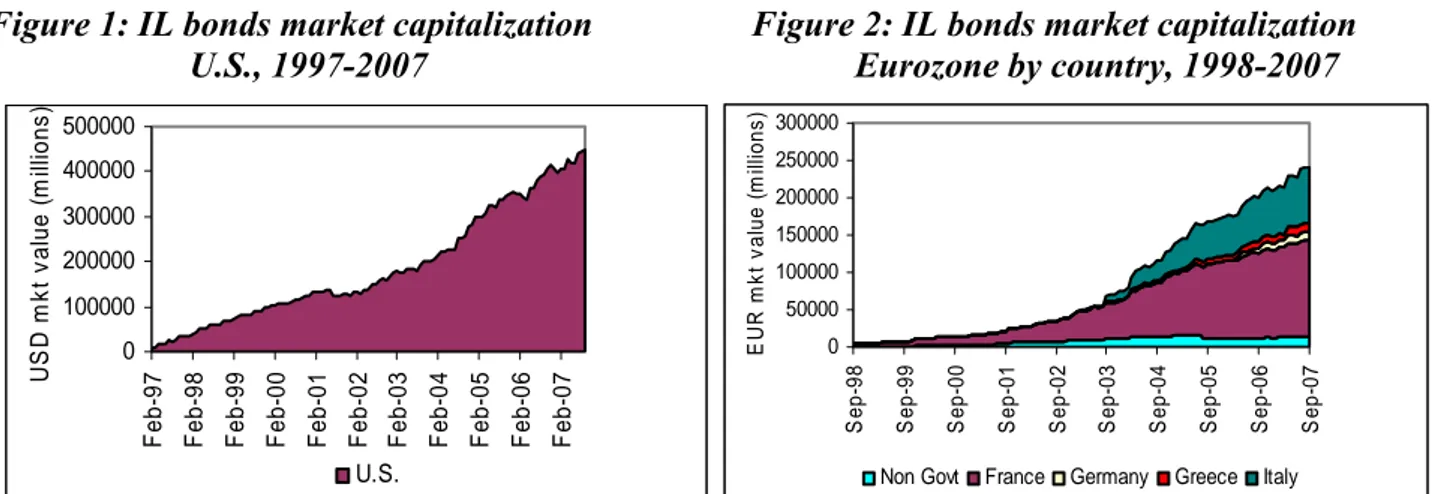
The market value of U.S. IL bonds has grown enormously, from $168 billion in 2002 to $446 billion in August 2007. Market capitalization of French linkers rose from €31.5 billion in 2002 to €129 billion in August 2007 (Figures 1 and 2 in Appendix 1).
The data cover the period from October 1, 1998 to August 31, 2007 for the eurozone, and from March 3, 1997 to August 31, 2007 for the U.S. Stripping market holidays out of the sample, we obtain a total of 2,294 and 2,666 observations, respectively. All indices include coupon or dividend returns. Figures 3 and 4 in Appendix 1 show the cumulative daily returns of the six asset classes, and Table 1 below displays their summary statistics. All returns have been tested for stationarity, with positive results (not reported here).
1
See “Barclays Inflation-Linked Bond Indices, Index Products”, Barclays Capital Research, 2006. 2
It represents more than 50% of the eurozone market. 3
Table 1: Descriptive statistics, U.S. and Eurozone
Daily returns in local currency
Nominal Bonds IL Bonds Equities
US (1997-2007) Average 0.03% 0.03% 0.04% Ann. Average 6.55% 6.55% 9.10% Median 0.03% 0.02% 0.05% Min -1.81% -1.43% -6.87% Max 1.61% 1.24% 5.73% Std Dev 0.40% 0.28% 1.13% Ann. Std. Dev. 6.30% 4.43% 18.00% Skewness -0.27 -0.15 -0.01 Kurtosis 1.45 2.34 3.05 Eurozone*(1998-2007) Average 0.02% 0.02% 0.04% Ann. Average 4.65% 5.09% 9.37% Median 0.02% 0.01% 0.08% Min -1.84% -1.29% -6.38% Max 1.33% 1.10% 6.35% Std Dev 0.32% 0.26% 1.29% Ann. Std. Dev. 5.06% 4.06% 20.42% Skewness -0.41 -0.29 -0.04 Kurtosis 1.93 2.26 2.82
* French data for IL bonds and nominal bonds
During our sample period, the average return on linkers was higher than that on nominal bonds in Europe (5.09% versus 4.65%), and equal to nominal bonds in the U.S. (6.55%). Theoretically, nominal bond returns should include compensation for the risk of unexpected future inflation: the inflation risk premium (Sarte (1998), Shen (1998), McCulloch and Kochin (2000)). Nominal bonds are thus expected to provide slightly higher returns and risks than IL bonds with similar maturities. In that context, the impressive performance of linkers compared to nominal bonds is surprising. It may be due to the sample period, which began with low supply and very high demand from institutional investors (insurance companies and pension funds) seeking protection from inflation, and to the presence of a liquidity premium (Shen (2006), Hordahl and Tristani (2007)). Over the entire study period, IL bonds exhibit lower volatility than nominal bonds in both the U.S. and Europe: 4.4% versus 6.3% in the U.S. and 4.1% versus 5.1% in France, consistent with the theoretical framework and previous findings (Hunter and Simon (2002)). In addition, equities provide a risk premium over Treasuries of
sharp difference between the two is that average nominal bonds returns were much lower in the eurozone than in the U.S.
3. Modeling time-varying correlation
3.1 Instability of correlations
Tables 2 and 3 present the unconditional correlation matrices calculated in the U.S. and the eurozone over the entire sample period. One oft-cited source of diversification provided by IL bonds is the fact that they exhibit negative correlation with other assets classes (especially equities) and moderate correlation with nominal bonds. In our sample, IL bonds display negative correlations with equities (-0.14 in the U.S., -0.24 in the eurozone), and very high correlations with nominal bonds (0.75 in the U.S., 0.70 in the eurozone).
Table 2: Correlation matrix, U.S., 1997-2007
Daily returns in local currency
Table 3: Correlation matrix, Eurozone, 1998-2007
Daily returns in local currency
Nominal Bonds IL Bonds Equities Nominal Bonds IL Bonds Equities
Nominal Bonds 0.75 -0.17 Nominal Bonds 100.00% 0.70 -0.25
IL Bonds -0.14 IL Bonds 93.51% -0.24
Equities 6.32% 30.37% 100.00% Equities -1.35% 8.63% 100.00%
As mentioned previously, the linkers market is relatively new, and many studies arguing for their strong diversifying power (Lamm (1998), Roll (2004)) refer to their early history. It is thus reasonable to wonder if, after 10 years of growth and change in the market, we will reach a different conclusion.
As a preliminary step, we split the full sample into two equal-length sub-periods: from the inception date to 2002, and from 2003 to 2007. The choice of dates may be debatable, but volume and turnover in this market clearly doubled after 2003, with growth in issuance, liquidity, and the number of market participants. Shen (2006) finds, for example, a decreasing liquidity premium after 2003 in U.S. TIPS, and Hordahl and Tristani (2007) cite high liquidity
premiums before that date. In Europe, 2003 coincides with the issuance of Italian and Greek IL bonds. Tables 4 to 7 present the correlation matrices for the two sub-samples.
Table 4: Correlation matrix, U.S., 1997-2002
Daily returns in local currency
Table 5: Correlation matrix, Eurozone, 1998-2002
Daily returns in local currency
Nominal Bonds IL Bonds Equities Nominal Bonds IL Bonds Equities
Nominal Bonds 0.67 -0.17 Nominal Bonds 100.00% 0.53 -0.20
IL Bonds -0.15 IL Bonds 93.51% -0.21
Equities 6.32% 30.37% 100.00% Equities -1.35% 8.63% 100.00%
Table 6: Correlation matrix, U.S., 2003-2007
Daily returns in local currency
Table 7: Correlation matrix, Eurozone, 2003-2007
Daily returns in local currency
Nominal Bonds IL Bonds Equities Nominal Bonds IL Bonds Equities
Nominal Bonds 0.88 -0.17 Nominal Bonds 100.00% 0.93 -0.34
IL Bonds -0.16 IL Bonds 93.51% -0.31
Equities 6.32% 30.37% 100.00% Equities -1.35% 8.63% 100.00%
We notice a relevant change in the nominal / IL bonds correlation since 2003. In the U.S., the correlation increases from 0.67 to 0.88. In France, the increase is even larger from 0.53 to 0.93. Correlations of nominal and IL bonds with equities increased less significantly, and remained completely stable in the U.S.
Volatilities also appear very different in the two sub-periods, as can be seen in Tables 8 and 9. Equity index volatility for the second period is roughly 0.6 times that for the first sub-period (which included the equity market crash), whereas nominal bond volatility decreases slightly in the second period in both areas. Again, a dramatic change occurred for IL bonds. Their volatility increased considerably–the volatility ratio between the second and first period is 1.79 in the U.S. and 1.55 in France–to levels comparable to nominal bonds (or even slightly higher in Europe).
Table 8: Volatilities and volatility ratio, U.S., 1997-2002 and 2003-2007
Daily returns in local currency
Table 9: Volatilities and volatility ratio, Eurozone, 1998-2002 and 2003-2007
Daily returns in local currency
Nominal Bonds IL Bonds Equities Nominal Bonds IL Bonds Equities 1997 - 2002 6.53% 3.15% 21.29% 1997 - 2002 5.5.75%% 3.08% 24.69% 2003 - 2007 6.00% 5.64% 12.71% 2003 - 2007 4.4.31%1% 4.79% 15.49% Ratio 0.92 1.79 0.60 Ratio 0.75 1.55 0.63
This preliminary analysis clarifies the problem of considering a covariance matrix calculated on the whole period. This may partly conceal the real-world situation, since correlations and volatilities are very unstable. Theχ2test by Engle and Sheppard (2001) allows us to test econometrically the null hypothesis of constant correlations against the alternative of dynamic conditional correlations. The results, reported in Tables 10 and 11 in Appendix 2,show strong rejection of the null hypothesis.In that context, the DCC-MVGARCH model will be of great interest, because it can cope with the varying correlations and volatilities over time.
3.2. Dynamic Conditional Correlation modeling
We apply the simplest form of the DCC-MVGARCH model first presented by Engle and Sheppard (2001) and Engle (2002). We consider the daily returns r of k asset classes and t
assume that the returns are conditionally normal4 with a mean of zero and covariance matrix
t H : 1 − t t I r ~N(0,Ht). t
H represents the conditional covariance matrix and can be decomposed as follows:
t t t
t D R D
H =
whereR is the conditional correlation matrix andt D =t h is a it kxk diagonal matrix whose elements are the conditional standard deviations of the returns on each asset class, typically thought of as univariate GARCH(p,q) models. The standardized residuals resulting from the univariate GARCH process are used to model the dynamic correlation.
The log likelihood for this estimator can be written:
4
(
)
∑
= − − − − + + + + − = T t t t t t t t t t t t r D D r R R D n L 1 1 ' ' 1 1 ' log log 2 ) 2 log( 2 1 π ε ε ε εThis log likelihood function can be considered as the sum of a volatility component Lv(θ) and a correlation component LC
( )
θ,φ : t t t t t v n D r D D r L (θ)= log(2π)+2log + ' −1 −1( )
θ φ ε'ε ε' 1ε log , =− t t + t + t t− C R R LThe DCC model maximizes the log likelihood in two steps. The first stage is to find
( )
{
θ}
θ =argmax LV
∧
, i.e. the coefficients of a GARCH (p,q) process applied to each asset class. In the second stage the correlation coefficients are estimated conditionally to the parameters estimated in the first stage likelihood:
⎭ ⎬ ⎫ ⎩ ⎨ ⎧ ⎟ ⎠ ⎞ ⎜ ⎝ ⎛∧ φ θ ι , max LC .
3.3. Estimation results
A preliminary analysis (not reported there) has been conducted to choose the best univariate GARCH process for our assets. Tables 12 and 13 in Appendix 3 display the estimates of GARCH parameters for each series. Looking at the significance of parameters and information criteria, the model selected is a GARCH (1,1) for the six asset classes. All series present a high degree of persistence (long memory of the process), although the autoregressive parameter is more pronounced for bonds than for equities. By contrast, equities demonstrate an innovation parameter which is higher than that for bonds, meaning that a volatility shock lasts longer in equity markets than in bond markets.
Figures 5 to 8 plot the estimated conditional volatilities. The greater volatility of equities is conspicuous with respect to the two bond indices. The recent period has been characterized by a relatively low-volatility environment for equities and decreasing volatility for bonds. Volatility peaks are detectable, coinciding with crises (Schwert (1989), Bekaert and Wu (2000), Caporale et al. (2000)).
Figure 5: Conditional volatility of equities,
U.S. Figure 6: Conditional volatility of equities, Eurozone
Figure 7: Conditional volatilities of nominal and IL bonds, U.S.
Figure 8: Conditional volatilities of nominal and IL bonds, Eurozone
Until 2003, consistent with theory, IL bonds were less volatile than nominal bonds. But curiously, since that date, IL bond volatility increased sharply, reaching levels almost identical to those of nominal bonds, and even slightly higher in Europe.
This phenomenon, which is scarcely documented in the academic literature, can probably be explained by the greater stability of inflation expectations (Kahn et al. (2002), Ahmed et al. (2004), Bernanke (2006), Aglietta et al. (2007)). This stability has led to more stable inflation breakevens5, and therefore to real interest rates moving almost in parallel with nominal rates. Accordingly, the volatility of IL bonds returns is bound to be identical to that of nominal bonds,
5
Inflation breakevens are expressed as the difference between the nominal rate (quoted on nominal bonds) and the real rate (quoted on IL bonds) of the same maturity. Breakeven measures the market’s inflation expectation, plus premiums linked to inflation risk and to the difference in liquidity between the nominal bond market and the IL bond market. 0% 2% 4% 6% 8% 10% 12% m a r-9 7 m a r-9 8 m a r-9 9 m a r-0 0 m a r-0 1 m a r-0 2 m a r-0 3 m a r-0 4 m a r-0 5 m a r-0 6 m a r-0 7
Nominal Bonds IL Bonds
0% 2% 4% 6% 8% 10% 12% Oc t-9 8 Oc t-9 9 Oc t-0 0 Oc t-0 1 Oc t-0 2 Oc t-0 3 Oc t-0 4 Oc t-0 5 Oc t-0 6
Nominal Bonds IL Bonds 0% 10% 20% 30% 40% 50% 60% M a r-97 M a r-98 M a r-99 M a r-00 M a r-01 M a r-02 M a r-03 M a r-04 M a r-05 M a r-06 M a r-07 Equities 0% 10% 20% 30% 40% 50% 60% Oc t-98 Oc t-99 Oc t-00 Oc t-01 Oc t-02 Oc t-03 Oc t-04 Oc t-05 Oc t-06 Equities
since the returns of both bond classes are dominated by their common component (Hordahl and Tristani (2007)).
The second stage of DCC-MVGARCH modeling is estimation of the dynamic conditional correlation. The parameter estimates of the selected specification, a DCC (1,1) 6, are presented in Tables 14 and 15 in Appendix 3. Figures 9 and 10 depict the estimated dynamic correlation between the six asset classes involved.
6
Alternative specifications (DCC(2.1), DCC(1,2), DCC(2,2), etc.) have been tested, but parameters were not significant and the log likelihood did not improve.
Figure 9: Conditional correlations between
nominal bonds, IL bonds and equities, U.S. between nominal bonds, IL bonds and Figure 10: Conditional correlations equities, Eurozone
The equity / nominal bond correlation declined significantly beginning in 1998, becoming almost always negative since that date. It is noteworthy that there is a strong analogy between the equity / nominal bond correlation and the equity / IL bonds correlation, especially since 2003. In theory, the correlation of IL bonds with equities should be weaker than that of nominal bonds with equities (Kothari and Shanken (2004)). In fact, nominal bonds and equities are both negatively impacted by unexpected inflation, while indexed bonds are positively impacted, given the negative relationship between inflation and real interest rates.
The most striking fact concerns the change of behavior of the correlation between indexed bonds and nominal bonds. Fluctuating around 60% before 2003, and relatively volatile, the correlation approaches 90% and is extremely stable after that date. Earlier studies (Lucas and
-1,0 -0,5 0,0 0,5 1,0 ma r-9 7 ma r-9 8 ma r-9 9 ma r-0 0 ma r-0 1 ma r-0 2 ma r-0 3 ma r-0 4 ma r-0 5 ma r-0 6 ma r-0 7
Nom Bonds,IL Bonds Nom Bonds, Equities IL Bonds, Equities -1.0 -0.5 0.0 0.5 1.0 Oc t-9 8 Oc t-9 9 Oc t-0 0 Oc t-0 1 Oc t-0 2 Oc t-0 3 Oc t-0 4 Oc t-0 5 Oc t-0 6
Nom Bonds,IL Bonds Nom Bonds, Equities
Quek (1998), Lamm (1998), Rudolph-Shabinsky and Trainer (1999)) showed that the correlation between the two markets should depend on whether nominal interest rate movements are more reflective of changes in real interest rates or changes in inflation expectations. Thus, when inflation expectations are moving the market more, IL bonds and nominal bonds tend to be less correlated, and when real rates vary, a higher correlation may be expected. The greater stability of inflation expectations could explain why real rates, while fluctuating in parallel with nominal rates, are much more highly correlated with inflation expectations. In addition, aspects of liquidity that are linked to the novelty of IL bonds may explain why their correlation was abnormally low at the beginning of the data series, when the indexed market was subject to significant supply / demand factors.
4. Consequences for Asset allocation
Our objective is to design optimal portfolios with monthly rebalancing, and to measure how their composition changes through time because of the movements in volatility and the correlation process observed in the previous section. The estimated conditional correlations and volatilities allow us to compute daily a conditional covariance matrix that can be used for portfolio optimization, with a standard mean-variance approach.
We consider a diversified portfolio composed of nominal bonds, IL bonds and equities, with the possibility of investing in a risk-free asset also. To examine how changes in the volatility and correlation structure affect the design of an optimal portfolio, we assume that the expected returns of each asset are constant and equal to long-term equilibrium expectations throughout the period under review. We can thus analyze changes in the portfolio’s optimal composition that are due entirely to variations in conditional volatilities and correlations.
The first step is to determine reasonable assumptions for expected long-term excess returns for the three asset classes relative to the risk-free rate. For both nominal and IL bonds, we consider three scenarios: (1) a baseline scenario of a 1.5% excess return over the risk-free rate, corresponding to the historic U.S. average since 1980, and two alternative scenarios: a more favorable one for bonds with an expected excess return of 2%, and a less favorable one with an excess return of only 1%. We also examine the sensitivity of thefindings to various alternative
assumptions, in particular the possibility of a positive inflation risk premium warranting higher expected returns for nominal bonds than for indexed bonds. This premium would compensate a nominal bond holder for the risk that inflation may be higher than expected. Historically, the inflation risk premium has fluctuated widely in response to economic conditions, both in the United States and in Europe. An abundant literature is devoted to estimating it (Berardi (2005), D’Amico et al. (2007), Durham (2006), Hördahl and Tristani (2007), Risa (2001), Shen (1998)), with estimates ranging from 0% to slightly over 1%. We therefore took three scenarios for this premium: 0%, 0.5% and 1%. Making these assumptions for nominal and IL bonds, we deliberately exclude the case of a highly inflationary scenario. Finally, we assume that equities earn an excess return of 4% over the risk-free rate, corresponding to the historical U.S. average. The purpose of this paper is not to study equity behavior in detail, so we use a single assumption for this asset class. Combining the three bond return assumptions and the three inflation risk premium assumptions, we construct nine possible expected return scenarios for the three asset classes, consistent with the hypotheses used by Kothari and Shanken (2004), thus enabling us to compare the results obtained in the two studies.
At every month-end we optimize our portfolios by maximizing the Sharpe ratio. We assume (1) that expected returns are equal to long-term expectations as defined in each of the nine scenarios, and (2) that the expected variance-covariance matrix is equal to the last conditional variance-covariance matrix estimated in section 3.
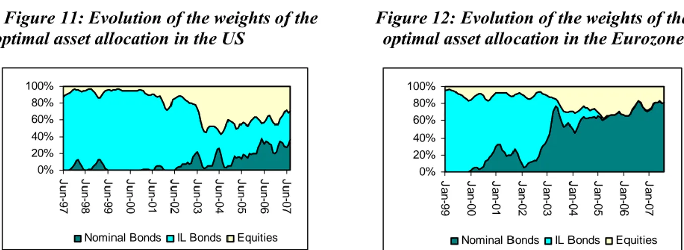
The following charts plot the changes in the weights of each of the three asset classes under our dynamic optimization, using two scenarios selected from the nine available. Figures 11 and 12 present the baseline case in which excess bond return is 1% and the inflation risk premium is nil in both the United States and Europe. Figures 13 and 14 present a more favorable scenario for nominal bonds in which the excess return is still 1% but the inflation risk premium is 0.5%, the average estimate in the literature. Tables 14 and 15 summarize optimizations carried out in the United States. They show the average dynamic optimal weights obtained from our monthly portfolio optimizations over the two sub-periods. Tables 16 and 17 show the same for Europe.
Figure 11: Evolution of the weights of the Figure 12: Evolution of the weights of the optimal asset allocation in the US optimal asset allocation in the Eurozone
Notes: Annualized expected excess return (over the risk-free rate) of Nominal Bonds, IL Bonds and Equities is equal to 1%, 1% and 4% respectively
Figure 13: Evolution of the weights of the Figure 14: Evolution of the weights of the optimal asset allocation in the US optimal asset allocation in the Eurozone
Notes: the annualized expected excess return (over the risk-free rate) of Nominal Bonds, IL Bonds and Equities is equal to 1%, 0.5% and 4% respectively.
0% 20% 40% 60% 80% 100% J un-97 J un-98 J un-99 J un-00 J un-01 J un-02 J un-03 J un-04 J un-05 J un-06 J un-07
Nominal Bonds IL Bonds Equities
0% 20% 40% 60% 80% 100% J an-99 J an-00 J an-01 J an-02 J an-03 J an-04 J an-05 J an-06 J an-07
Nominal Bonds IL Bonds Equities
0% 20% 40% 60% 80% 100% J an-99 J an-00 J an-01 J an-02 J an-03 J an-04 J an-05 J an-06 J an-07
Nominal Bonds IL Bonds Equities 0% 20% 40% 60% 80% 100% Ju n -9 7 Ju n -9 8 Ju n -9 9 Ju n -0 0 Ju n -0 1 Ju n -0 2 Ju n -0 3 Ju n -0 4 Ju n -0 5 Ju n -0 6 Ju n -0 7
Table 14: Optimal asset allocation weights U.S. 1997-2002
Excess Return Nominal Bonds
1% 1.5% 2%
IRP
Nominal
Bonds IL Bonds Equities
Nominal
Bonds IL Bonds Equities
Nominal
Bonds IL Bonds Equities
0% 3 86 9 2 89 6 1 91 5
0.5% 28 52 17 14 74 10 8 83 7
1.0% 67 1 30 49 32 16 30 57 10
Table 15: Optimal asset allocation weights U.S
2003-2007
Excess Return Nominal Bonds
1% 1.5% 2%
IRP
Nominal
Bonds IL Bonds Equities
Nominal
Bonds IL Bonds Equities
Nominal
Bonds IL Bonds Equities
0% 19 40 41 22 45 33 24 48 28
0.5% 55 1 44 61 3 36 63 7 30
1.0% 55 0 45 64 0 36 69 0 31
Table 16: Optimal asset allocation weights Eurozone
1998-2002
Excess Return Nominal Bonds
1% 1.5% 2%
IRP
Nominal
Bonds IL Bonds Equities
Nominal
Bonds IL Bonds Equities
Nominal
Bonds IL Bonds Equities
0% 13 78 10 12 81 7 12 82 6
0.5% 40 44 16 28 62 10 23 70 7
1.0% 75 0 25 62 23 15 43 48 10
Table 17: Optimal asset allocation weights Eurozone 2003-2007
Excess Return Nominal Bonds
1% 1.5% 2%
IRP
Nominal
Bonds IL Bonds Equities
Nominal
Bonds IL Bonds Equities
Nominal
Bonds IL Bonds Equities
0% 66 8 26 70 8 22 73 8 19
0.5% 74 0 26 78 0 22 80 1 19
1.0% 74 0 26 78 0 22 81 0 19
Notes: Annualized expected excess returns are given in excess of the risk-free rate. They are kept constant for equities at 4%. IRP stands for Inflation Risk Premium. Optimal asset allocation weights represent the averages of the dynamic optimal portfolio weights in the two periods.
These results clearly show the break in optimal portfolio structure in 2003, regardless of the assumptions used. Before 2003 a significant portfolio weight in IL bonds was appropriate, but
returned as much as nominal bonds. The weight of IL bonds is about 80% on average before 2003, but thereafter it decreases to about 40% in the United States and less than 10% in Europe. A more favorable hypothesis for nominal bonds versus IL bonds, i.e. an inflation risk premium of 0.5%, reduces the weight even further, from about 60% to 0. These results shed interesting light on the work of Kothari and Shanken (2003), which applies similar assumptions to selected optimizations but on a data series ending in 2003. Our results for the first period are in fact in line with the authors’ findings, but we show how much the situation has evolved since 2003, and how much IL bonds’ diversifying power has changed.
Before 2003 high expected bond returns (2%) mean that, for any expected inflation risk premium, a substantial proportion of IL bonds in the portfolio is always optimal. Of course, this optimal weight decreases with the premium (around 90% in the United States and 80% in Europe for nil premium, 80% in the United States and 70% in Europe for a 0.5% premium, 60% in the United States and 50% in Europe for a 1% premium). After 2003 the diversifying power of IL bonds changes the situation drastically, with unchanged expected returns. It is not worthwhile including a substantial proportion of IL bonds in a portfolio (around 50% in the United States, 10% in Europe) unless the inflation risk premium is nil. In all other cases, it is not optimal to include IL bonds at all.
It is worth noting the difference in results between the United States and Europe. The optimal weight of IL bonds in a portfolio is always greater in the United States than in Europe. Before 2003 this is explained by the wider volatility spread between nominal and IL bonds in the US (3.1% for IL versus 6.5% for nominal) than in Europe (3.1% versus 5.7%), giving an advantage to IL bonds. After 2003 the phenomenon is accentuated by the fact that the volatility of IL bonds remains slightly lower than that of nominal bonds in the United States (5.6% versus 6%), while it rises in Europe (4.8% versus 4.3%). Another factor has also tended to amplify the differences between the two regions: the correlation between nominal bonds and IL bonds is becoming higher in Europe (93%) than in the United States (88%). Therefore, IL bonds seem to offer slightly greater diversifying power in the United States.
This exercise shows how important it is to consider the variance-covariance matrix that best represents the regime that will take place in the future. In the case of IL bonds, the structure of volatilities and correlations has changed completely because inflation expectations have stabilized since 2003 and the market has become more liquid. This change implies significant
modifications to the optimal composition of an overall portfolio. Since 2003 IL bonds have become almost substitutable for nominal bonds for diversification purposes in an overall portfolio. They have the same risk and almost the same correlations. Thus, IL bonds should not be introduced in a global portfolio for diversification reasons alone, as was the case before 2003. Whether they should be introduced now will depend more on investors’ expectations of the relative excess returns of both nominal and IL bonds, bearing in mind that they provide a hedge against inflation risk.
In case of an unexpected surge in inflation, it is highly probable not only that expected returns would change but that the correlation structure would also vary, reverting to a pattern to that closer pre-2003. Under these conditions, the effects of diversifying between IL and nominal bonds may increase. IL bonds would then become attractive again, both because they would outperform nominal bonds and because they would once again be able to diversify an overall portfolio.
5. Conclusion
We have proposed a method for estimating conditional correlations and volatilities between IL bonds, nominal bonds and equities, in the United States and Europe for the period 1997 – 2007, using a DCC-MVGARCH model (Engle (2002)).
The results have enabled us to show that the dynamics of correlations and volatilities have changed radically in recent years. The volatility of IL bonds, which used to be weaker than that of nominal bonds, in keeping with the theory, increased sharply to levels that are now identical to nominal bonds (or even higher in Europe). Indexed bonds have become strongly correlated with nominal bonds, thus losing a large measure of both their diversifying power and their attractiveness for an overall portfolio.
These results shed new light on the subject, in contrast to the earlier literature, which highlighted the strong diversifying power of IL bonds during their first years in existence (Lamm (1998), Roll (2004), Kothari and Shanken (2004), Mamun and Visaltanachoti (2006a)).
possible that a lack of liquidity and a supply / demand imbalance, amid strongly intensifying demand from institutional investors for IL bonds in recent years, made the early price history unrepresentative, and misrepresented the decorrelating power of IL bonds in relation to nominal bonds. Another factor that also played a definite role was the fairly strong decline in inflation expectations and their volatility, in a context of credible inflation-fighting monetary policies and in a more favorable economic environment for low, stable inflation.
Monthly portfolio optimization carried out since 1997, using our dynamic conditional correlation and volatility estimates and constant expected excess returns, clearly shows the decreasing weight that would have been allocated to IL bonds in an optimal allocation. Before 2003 the optimal weight of IL bonds in a portfolio was higher than that of nominal bonds. After 2003, considering the same hypothesis for expected returns, the weight of IL bonds declined sharply. This study shows that in terms of diversification, IL and nominal bonds are now almost substitutable: they have more than 90% correlation with nominal bonds, roughly the same correlation with equities and same volatility as nominal bonds. It is clear that portfolio managers must today take these changes into account.
If diversification purpose could be a sufficient reason for introducing IL bonds before 2003, it is no more the case. The decision to introduce them will now depend solely on investors’ expectations for the relative excess returns of both nominal and IL bonds, but also their inflation risk aversion, given the fact that IL bonds provide a hedge against inflation risk.
An unexpected surge of high inflation would change the picture completely. The expected return on IL bonds may become much higher than that on nominal bonds (Roll (2004), Mamun and Visaltanachoti (2006b)). Furthermore, the higher variability of inflation expectations would certainly change the correlation structure of IL bonds relative to other assets, restoring much of IL bonds’ pre-2003 diversifying power in an overall portfolio. One interesting direction for future research would be to determine the extent to which a future, unexpected increase in inflation could modify the optimal allocation. Finally, now that most developed countries issue IL bonds, a comparative study of these markets would be highly instructive and would probably add to our understanding of the nature and causes of the changes that occurred in the United States and Europe in 2003.
References
Ahmed, S., Levin A. and Wilson (2004), “Recent US Macroeconomic Stability: Good Policies, Good Practices or Good Luck,” Review of Economics and Statistics, 86(3), 824-832.
Aglietta M., Berrebi M. and Cohen-Benamran A. (2007), “La mutation des taux d’intérêt américains face à la globalisation”, Expertises 5-2007, Groupama Asset Management.
Bekaert, G. and Wu, G. (2000), “Asymmetric volatility and risk in equity markets” Review of Financial Studies, 13,1, 1-42.
Berardi A., (2005), “Real Rates, expected inflation and inflation risk premia implicit in nominal bond yields”, Financial Management Association Conference Proceedings, Sienna 2005.
Bernanke, B.S. (2006), “Reflections on the Yield Curve and Monetary Policy,” speech to the Economic Club of New York, 20 March.
Billio, M. and Caporin, M. (2004), “A generalized Dynamic Conditional Correlation model for portfolio risk evaluation,” GRETA Working Paper, 04-05.
Billio, M. and Caporin, M. (2005), “Multivariate Markov Switching Dynamic conditional Correlation GARCH representations for contagion analysis,” GRETA Working Paper, 05-02.
Campbell, J.Y. and Shiller, R.J. (1996), “A Scorecard for Indexed Government Debt,” NBER Working Paper, 5587.
Campbell, J.Y and Viceira, L. (2002), “Strategic Asset Allocation: Portfolio Choice for Long Term Investors,” Clarendon Lectures in Economics, New York, Oxford University Press.
Caporale, G.M., Pittis, N. and Spagnolo, N. (2000), “Volatility Transmission and Financial Crises,” Econometric Society, available at http://www.econometricsociety.org.
Cappiello, L., Engle, R. F. and Sheppard, K. (2003), “Asymmetric Dynamics in the Correlations of Global Equity and Bond Returns”, ECB Working Paper, 204.
D’Amico S., Kim D.H., Wei M. (2007), “Tips from Tips : The Informational Content of Tresury Inflation-Protected Security Prices”, Federal Reserve Bank of Dallas Working Paper, 2007-07.
Durham J.B. (2006), “An Estimate of the Inflation Risk Premium Using a Three-Factor Affine Term Structure Model”, Federal Reserve Bank of Washington, Finance and Economics Discussion Series, 2006-42.
Engle, R. F. (2002) “Dynamic Conditional Correlation – A simple class of multivariate GARCH models,” Journal of Business and Economics Statistics, 20(3), p.339-350.
Engle, R. F. and Sheppard, K. (2001), “Theoretical and Empirical Properties of Dynamic Conditional Correlation Multivariate GARCH,” University of California, San Diego, Department of Economics Discussion Paper, 2001-15.
Hördahl, P. and Tristani, O. (2007), “Inflation risk premia in the term structure of interest rates,” ECB Working Paper, 734.
Hunter, D. and Simon, D. (2005), “Are TIPS the “Real” Deal? A Conditional Assessment of Their Role in a Nominal Portfolio,” Journal of Banking and Finance, 29, p. 347-368.
Kahn, J.A., McConnell, M.M. and Perez-Quiros, G. (2002), “On the Cause of the Increased Stability of the US Economy,” Federal Reserve Bank of New York, Economic Policy Review, 8(1), 183-203.
Kearney, C. and Potì, V. (2003), “DCC-GARCH modelling of Market and Firm-Level Correlation Dynamics in the Dow Jones Eurostoxx50 Index”, School of Business Studies, Trinity College Dublin.
Kothari, S.P. and Shanken, J. (2004), “Asset Allocation with Inflation Protected Bonds”, Financial Analyst Journal, January-February, p. 54-70.
Lamm, R. M. (1998), “Asset Allocation Implications of Inflation Protection Securities,” Journal of Portfolio Management, 24, p. 93-100.
Mamun, A. and Visaltanachoti, N. (2006a), “Diversifying Benefits of Treasury Inflation Protected Securities: an Empirical Puzzle,” available at SSRN, http://ssrn.com/abstract_id=663669.
Mamun, A. and Visaltanachoti, N. (2006b), “Inflation Expectation and Asset Allocation in the Presence of an Indexed Bond,” available at SSRN: http://ssrn.com/abstract=907147.
McCulloch, J.H. and Kochin, L.A. (2000), “The Inflation Premium Implicit in the US Real and Nominal Term Structures of Interest Rates,” Ohio State University Economics Dept Working Paper, 98-12, revised in September 2000.
Risa S. (2001), “Nominal and Inflation Indexed Yields : Separating Expected Inflation and Inflation Risk Premia”, Available at SSRN: http://ssrn.com/abstract=265588.
Roll, R. (2004), “Empirical TIPS,” Financial Analyst Journal, 60(1), January-February, p. 31-53.
Sarte, P.G. (1998), “Fisher’s Equation and the Inflation Risk Premium in a Simple Endowment Economy,” Federal Reserve Bank of Richmond Economic Quarterly, 84(4), Fall 1998.
Schwert, G.W. (1989), “Business Cycles, Financial Crises and Stock Volatility,” NBER Working Paper, 2957, May.
Shen P. (1998), “How Important is the Inflation Risk Premium,” Federal Reserve Bank of Kansas City, Economic review, fourth quarter 1998.
Shen, P. (2006), “Liquidity Risk Premiums and Breakeven Inflation Rates,” Federal Reserve Bank of Kansas City, Economic review, Second Quarter 2006.
Van Dijk, D., Munandar, H. and Hafner, C.M. (2006), “The Euro introduction and Non-Euro Currencies,” Medium Econometrische Toepassingen, 14(1).
Appendix
Appendix 1
Figure 1: IL bonds market capitalization Figure 2: IL bonds market capitalization U.S., 1997-2007 Eurozone by country, 1998-2007
Source : Barclays
Figure 3: Cumulative daily returns, Figure 4: Cumulative daily returns, U.S., 1997 – 2007 Eurozone, 1998 - 2007 Source : Barclays 0 100000 200000 300000 400000 500000 Fe b -9 7 Fe b -9 8 Fe b -9 9 Fe b -0 0 Fe b -0 1 Fe b -0 2 Fe b -0 3 Fe b -0 4 Fe b -0 5 Fe b -0 6 Fe b -0 7 US D m k t v a lue (m ill ions ) U.S. 0 50000 100000 150000 200000 250000 300000 S ep-98 S ep-99 S ep-00 S ep-01 S ep-02 S ep-03 S ep-04 S ep-05 S ep-06 S ep-07 E U R m k t v a lue ( m il lions )
Non Govt France Germany Greece Italy
90 110 130 150 170 190 210 230 250 Ma r-9 7 Ma r-9 8 Ma r-9 9 Ma r-0 0 Ma r-0 1 Ma r-0 2 Ma r-0 3 Ma r-0 4 Ma r-0 5 Ma r-0 6 Ma r-0 7
Nominal Bonds IL Bonds Equities
70 90 110 130 150 170 190 210 230 Oc t-9 8 Oc t-9 9 Oc t-0 0 Oc t-0 1 Oc t-0 2 Oc t-0 3 Oc t-0 4 Oc t-0 5 Oc t-0 6
Appendix 2
Table 10: Constant conditional correlation test*
U.S., 1997-2007
*Engle and Sheppard (2001) Ho:Rt =R∀t∈T
Table 11: Constant conditional correlation test*
Eurozone, 1998-2007
Appendix 3
Table 12: Univariate GARCH parameters estimates, U.S., 1997-2007
ω α β
Nominal Bonds 1.84E-08 0.02 0.97
(1.12E-08) (0.004) (0.003)
IL Bonds 2.61E-08 0.033 0.963
(8.94E-09) (0.009) (0.010)
Equities 1.32E-06 0.079 0.912
(4.99E-07) (0.012) (0.013)
α represents the ARCH term,β the GARCH term,ω the constant of the variance equation. Standard errors in parenthesis.
Table 13: Univariate GARCH parameters estimates, Eurozone, 1998-2007
ω α β
Nominal Bonds 4.07E-08 0.03 0.97
(8.22E-09) (0.007) ((0.007)
IL Bonds 1.39E-08 0.044 0.956
(1.83E-08) (0.008) (0.009)
Equities 1.08E-06 0.068 0.925
(5.70E-07) (0.014) (0.015)
α represents the ARCH term,β the GARCH term,ω the constant of the variance equation. Standard errors in parenthesis.
2
χ value P- value χ2 value P- value
Table 14: DCC (1,1) parameters estimates, US, 1997-2007
Parameters Estimates St.Dev. z-stat
α 0.016 0.0028552 5.584
β 0.984 0.0029852 329.551
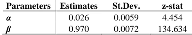
Table 15: DCC (1,1) parameters estimates, Eurozone, 1997-2007
Parameters Estimates St.Dev. z-stat
α 0.026 0.0059 4.454