Quality assessment of speckle patterns for digital image correlation
D. Lecomptea,*, A. Smitsb, Sven Bossuytb, H. Solb, J. Vantommea, D. Van Hemelrijckb, A.M. Habrakenc aDepartment of Materials and Construction, Royal Military Academy, Avenue de la Renaissance 30, 1000 Brussels, Belgium bMechanics of Materials and Constructions, Vrije Universiteit Brussel, Pleinlaan 2, 1050 Brussels, Belgium
cMechanics of Materials and Structures, Université de Liège, Chemin des Chevreuils 1,, 4000 Liège, Belgium
Abstract
Digital image correlation (DIC) is an optical-numerical full-field displacement measuring technique, which is nowadays widely used in the domain of experimental mechanics. The technique is based on a comparison between pictures taken during loading of an object. For an optimal use of the method, the object of interest has to be covered with painted speckles. In the present paper, a comparison is made between three different speckle patterns originated by the same reference speckle pattern. A method is presented for the determination of the speckle size distribution of the speckle patterns, using image morphology. The images of the speckle patterns are numerically deformed based on a finite element simulation. Subsequently, the displacements are measured with DIC-software and compared to the imposed ones. It is shown that the size of the speckles combined with the size of the used pixel subset clearly influences the accuracy of the measured displacements.
Keywords: Digital image correlation; Speckle pattern; Displacement field
1. Introduction
The identification of the mechanical properties of different materials requires appropriate strain measuring techniques. This is especially true for loading conditions which create complex heterogeneous deformation fields. Full-field measurement techniques and the digital image correlation (DIC) technique in particular are suitable to tackle this challenge. This technique—also referred to as white light speckle technique—is an optical-numerical full-field measuring technique, which offers the possibility to determine in-plane displacement fields at the surface of objects under any kind of loading, based on a comparison between images taken with a digital charge coupled device (CCD) camera at different load steps. This technique has been used in various
technological domains and many of its applications have been reported [1-6]. The capacity of the technique to measure non-homogeneous deformation fields has been described [7] as well as its limits and the accuracy of the measured displacements [8, 9].
The aim of the present paper is to study the efficiency of a speckle pattern and its influence on the measured in-plane displacements with respect to the subset size. It has already been shown [10-13] that the subset size is always a critical parameter in the correlation process. However, the particularity of this study is that the images representing the different speckle patterns and simulating an actual experiment are numerically deformed. This approach offers two main advantages. On the one hand, it allows dealing with only one variable, being the aspect of the speckle pattern; on the other hand, it allows comparing the displacements measured by the DIC technique with the numerically imposed displacements. This procedure has the advantage that possible variations of illumination of the pictured surface, instabilities of the experimental set-up and optical aberration do not interfere.
Three different pictures are taken of the same randomly painted speckle pattern. Each picture is taken with a different zoom, yielding three speckle patterns which are different by the size of the speckles, as if it concerned an actual experiment. Subsequently, each image undergoes a numerically controlled deformation, which is measured with the DIC software. Two types of deformation are imposed, a homogeneous deformation with a constant strain value in both directions and a heterogeneous deformation; both being based on the result of a finite element simulation.
2. DIC
2.1. Principle
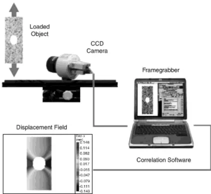
The DIC technique allows studying qualitatively as well as quantitatively the mechanical behaviour of materials under certain loading conditions. Each picture taken with a CCD camera corresponds to a different load step. The camera uses a small rectangular piece of silicon, which has been segmented into 1024 × 1280 arrays of individual light-sensitive cells, also known as photo-sites or pixels. Each pixel stores a certain grey scale value ranging from 0 to 255, in accordance with the intensity of the light reflected by the surface of the tested specimen. Two images of the specimen at different states of deformation are compared by using a pixel and its signature in the undeformed image, and searching for the pixel in the deformed image in order to maximize a given similarity function. In most cases, this function is based on a least-squares formulation. The signature of a pixel can be anything that discriminates it among any other pixel signature and can be the pixel grey-value, the grey-value derivatives or the pixel colour. In this case, the pixel grey-value is used. A single grey-value is not a unique signature of a pixel; hence, neighbouring pixels are used in practice. Such a collection of pixels is called a subset or correlation window. The displacement result, expressed in the centre point of the subset, is an average of the displacements of the pixels inside the subset. The step size defines the number of pixels over which the subset is shifted in x-and y-direction to calculate the next result. The size of a subset can be, e.g. 7x7, 11 × 11, 15 × 15 pixels, etc.; the step size can be 3, 5, 7 pixels, etc. The uniqueness of each signature is only guaranteed if the surface has a non-repetitive, isotropic, high-contrast pattern. Random textures of speckle patterns fulfil this constraint and can be obtained by an arbitrary speckle pattern that is applied onto the object surface, or that is offered by the texture of the specimen's material. Possible matches at several locations are checked and a similarity score (correlation function) is used to grade them. A classic correlation function using the sum of the squared differences of the pixel values is used. The image correlation routine allows locating every subset of the initial image in the deformed image. Subsequently, the software determines the displacement values of the centres of the subsets, which yields an entire displacement field. Fig. 1 depicts the sequence of taking a picture of an object before and after loading, storing the images onto a PC through a frame grabber, performing the
correlation of both images—i.e. locating the different undeformed subsets in the deformed image—and, finally, calculating the corresponding displacement of the centres of the subsets, which finally yields the desired displacement field.
2.2. Influence of the speckle pattern
The measured displacement results are influenced by the measurement system, the lighting conditions and the speckle pattern. As for the measurement system itself, three main elements can be distinguished: the lenses, the CCD camera and the correlation software. The lenses are responsible for conveying the beam of light, reflected by the object's surface towards the light sensitive cells of the CCD. The cells translate the incident light into voltage levels, which are scaled between 0 and 255. These values are then stored into a matrix with the same number of elements as the amount of light sensitive cells. The final step in the measurement process is the digital image correlation routine, in which two parameters are predominant—the nature of the speckle pattern and the size of the subset.
In the present paper, only these two parameters are studied. This allows avoiding any experimental errors. The purpose is to look at the influence of the nature of the speckle pattern on the measured displacements. To this end, finite element simulated displacement fields are used.
3. Creation of the different speckle patterns
The particularity of the displacement field, which is used for the evaluation of the speckle patterns, is that it is originated by a numerically deformed image. Firstly, a speckle pattern is randomly sprayed on a flat white surface. Several attempts were made to obtain an evenly distributed pattern of black paint drops. The same procedure is used in different studies in the case of actual experiments [14-19]. Three different images with a randomly chosen size of 250 × 500 pixels are extracted from this speckle pattern. The first image is taken from a given distance of the speckle pattern (Fig. 2b), yielding speckle pattern (b) with medium speckles. Fig. 2a covers an area which is twice as large as the area covered by Fig. 2b, but uses the same number of pixels. In this way speckle pattern (a) is created, featuring the small speckles. Finally, Fig. 2c shows speckle pattern (c) representing the large speckles. Fig. 2c represents half the size of the area pictured by Fig. 2b, but once again using only 250 × 500 pixels. The main difference between the three new images is thus the overall (and random) size of the black dots. It is the influence of this particular aspect that is studied in the present paper.
Fig. 1. Working principle of the DIC system.
Fig. 2. Sprayed speckle pattern with three different zooms yielding the three new reference speckle patterns.
4. Characterisation of the speckle patterns
4.1. Principle
To be able to characterise the speckle patterns more quantitatively, a method to calculate the speckle size distribution of a given pattern, based on image morphology, will be presented in this paragraph.
Morphology is a technique of image processing based on shapes. The value of each pixel in the output image is based on a comparison of the corresponding pixel in the input image with its neighbours. By choosing the size and shape of the neighbourhood, one can construct a morphological operation that is sensitive to specific shapes
in the input image. The operation consists in consecutively eroding and dilating the image. More detailed information can be found in [20]. In the present case, a circular shape is used with different radii. The objective is to locate the speckles with a radius that is superior to a given value. By performing this operation for different radius values, a speckle size distribution corresponding to the given pattern can be formulated.
4.2. Morphology study of a given speckle pattern
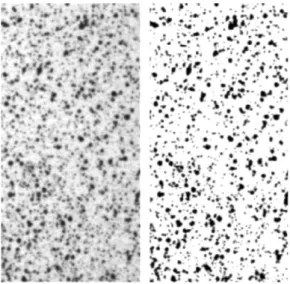
As an example, the speckle size distribution of speckle pattern (a) will be determined. The morphological technique yields the best results for binary images. Therefore, the chosen speckle pattern is firstly transformed into a black and white image. This is done by selecting a given grey value and turning every pixel with a higher grey value into a white pixel and every pixel with a lower grey value into a black pixel. In this way, an image is obtained in which the speckles are clearly delimited (Fig. 3).
Subsequently, the Matlab function "imopen" is used to locate the speckles with a mean radius larger than consecutively 10, 8, 6, 4 and 2 pixels. The result of this operation is shown in Fig. 4. At this time it is possible to calculate the distribution of the different speckle sizes. Therefore, the number of black pixels in the reference binary image is divided by the total number of pixels. This yields the "speckle covering" of the image. For speckle pattern (a) this ratio is about 15%. This quantity is practically the same for the three speckle patterns, which is logical since they actually represent the same speckle pattern.
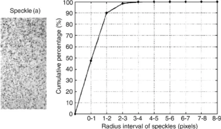
Next, the total number of black pixels is counted in the first image of Fig. 4, representing the speckles with a radius larger than 10 pixels. The same is done for the rest of the images in Fig. 4. Each time the total number of black pixels is decreased by the number of black pixels in the previous image. This makes it possible to generate a curve representing the cumulative speckle covering by speckles within a given radius interval. The result for speckle pattern (a) is shown in Fig. 5. The result for speckle pattern (b) and (c) is shown, respectively, in Figs. 6 and 7.
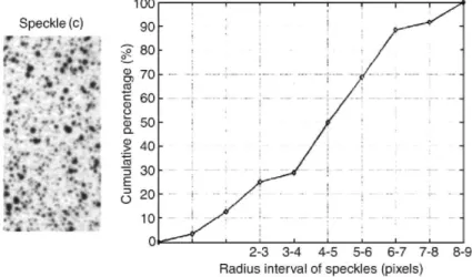
For speckle pattern (b) most speckles have a radius between 0 and 5 pixels. In the case of speckle pattern (a) the most frequent radii lie between 0 and 3 pixels, and for speckle pattern (c) between 3 and 7.
Fig. 4. Location of speckles with a diameter larger than respectively 10, 8, 6, 4 and 2 pixels.
Fig. 5. Cumulative percentage of speckles within a given radius interval for speckle pattern (a).
5. Finite element-based deformation of images
The images of the three speckle patterns are numerically deformed as to simulate a heterogeneous or a
homogeneous deformation. The deformation is based on a finite element simulated displacement field which is used afterwards as a reference for comparison of the displacements determined by DIC.
To obtain a heterogeneous deformation field, a circular part is numerically taken out of the centre of the images in order to simulate the surface of a perforated specimen (Fig. 8). Subsequently, a finite element analysis of a tension test of the specimen is performed (Fig. 8, middle). The obtained nodal displacement field (Fig. 8, right) is used to deform the original image. The result can be considered as a picture taken after loading of the real specimen, but without experimental errors. A DIC technique is used to compare the initial and the deformed image and to calculate the resulting displacement field.
The size of the images is 250 × 500 pixels. The size of the pixels is chosen to be equal to 100µm/pixel.
Therefore, the size of the finite element model is 25mm×50mm. The diameter of the hole is chosen to be 10 mm. The applied boundary conditions for the finite element simulation are a fixation of the top of the specimen, and a uniform displacement of 1 mm for the bottom of the specimen.
A grey value image can be seen as a matrix filled with integer values between 0 and 255. Every element of the matrix represents the grey value of a single pixel. To numerically deform an image, one has to start with an empty matrix with slightly adapted dimensions, depending on the type of deformation. This is because the deformed image will contain more or less pixels than the initial image. Firstly, the centres of the pixels in the deformed image have to be located in the deformed mesh. This is possible because the coordinate system is identical for both the deformed image and the finite element model, and because the nodal displacements are all known. Using the interpolation functions of the triangular elements, it is possible to determine the displacement components in the centre of every pixel. This also means that the initial position of the pixel can be traced back in the reference image by subtracting its displacement. Most likely, the initial position of a pixel from the deformed image is not located in the centre of a pixel of the initial image (Fig. 9). Therefore, it is necessary to
interpolate the grey values of the pixels in a given region around the initial position (box around initial position in Fig. 9). When the same procedure is followed for every pixel, the entire deformed image is finally constructed.
Fig. 6. Cumulative percentage of speckles within a given radius interval for speckle pattern (b).
Fig. 7. Cumulative percentage of speckles within a given radius interval for speckle pattern (c).
The same principle is used for the creation of a homogeneous deformation field. For reasons of simplicity, the Poisson's coefficient is chosen as equal to zero, so as to obtain a displacement component in the x-direction equal to zero as well. This means that only a linearly varying displacement component is present in the y-direction, which yields a constant strain value in that direction.
6. Evaluation of the displacements obtained with the different speckle patterns
6.1. Methodology
The reference images of the three speckle patterns and the corresponding deformed images can be considered as if they were generated by an actual experiment. Figs. 10 and 11 show the difference between the imposed (FEM-based) displacements and the measured displacements with the DIC software. This is elaborated for both homogeneous and heterogeneous deformation fields. Three different subset sizes—13 × 13, 23 × 23 and 33 × 33 pixels, respectively, small, medium and big subset—are used in the image correlation process. The results are presented in the form of histograms. The x-axis represents the difference between the imposed displacements and the DIC-calculated displacements in the horizontal direction. The y-axis represents the number of data points in which a given difference is present. Only the vertical displacement component is shown. Identical characteristics are found for the horizontal displacement fields. The imposed and measured displacements are compared in ± 3000 locations, arranged like a grid within the displacement field. For the understanding of the plots one should keep in mind the following remarks:
• The higher and the narrower the central peak, the better the correspondence between the imposed and the calculated displacements, thus the more accurate the results are.
• All the images are numerically treated in the same way. The difference in displacements is, therefore, only related to the speckle and the subset size.
Fig. 9. From the determination of the grey value of a single pixel in the deformed image, to the entire deformed
image.
6.2. Homogeneous displacement field
A first and important observation is that the larger the subset, the more accurate the measured displacements. This is shown by the narrowing of the peak for increasing subset sizes, and it is true for the three speckle types. The reason for this is that the information content is more important in the larger subsets. This means that in the case of a homogeneous displacement field, the information can be smoothened inside the subset, which
obviously leads to more accurate results.
A second observation is that in the case where the small subset is used, Fig. 10 shows that a most precise result is obtained with the smallest speckles, followed by the medium and large speckles. When using the medium subset the best result is obtained with the large speckles. In that case the difference between the small and medium speckles is negligible. In the last case, where the large subset is used, it is clear that the large speckles yield the
most precise results, followed by the medium and small speckles. If the best result is achieved by the large speckles, in the case where a medium subset is used, it is probable that in the case of a large subset the speckles can be even larger.
Fig. 10 clearly shows that the speckle size has to be compatible with the size of the subset. Furthermore, the size of the subset has to be adapted to the type of deformation. It is clear that in the case of homogeneous
deformation, the large subset size in association with the large speckles delivers the best results.
Fig. 10. Difference between the imposed and DIC-calculated displacement components or a homogeneous
displacement field as a function of the speckle pattern and the subset size.
6.3. Heterogeneous displacement field
In comparison to the results for the homogeneous displacement field, the peaks in Fig. 11 for the heterogeneous displacement field are broader. This means that the measured displacements are less accurate. The displacement field is more complex and thus less easily measurable, independent of the subset size. However, the same influence of the speckle size as for the homogeneous deformation is noticeable. When using small subsets, the speckle pattern with the larger speckles yields the most inaccurate results, which is shown by the broad peak. The best results in that case are obtained with speckle pattern (a) representing the small speckles.
The situation changes when using the medium and large subsets. In those cases the best results are obtained for speckle pattern (c). The choice leading to the most accurate results in the case of the present heterogeneous displacement field would be speckle pattern (c).
6.4. Relation between subset size and mean speckle size
The mean speckle size for the three different speckle patterns can be calculated based on the analysis of the speckle size distribution. The relation between the subset size and the mean speckle size, yielding the most accurate displacement results, is shown in Table 1.
Table 1: Mean speckle size for the three subset sizes
Subset size (in pixels) Mean speckle size (diameter in pixels)
Small—13 × 13 3
Medium—23 × 23 10
Big—33 × 33 >10
The results in Table 1 cannot yet be considered as the absolute reference. They are, strictly spoken, only valid for the cases studied in the present paper. More systematic research must be conducted to verify if these conclusions are generally valid or not.
Fig. 11. Difference between the imposed and DIC-calculated displacement components for a heterogeneous
7. Conclusion
In the present paper, the accuracy of the digital image correlation technique is studied in function of the nature of the speckle pattern—i.e. the mean speckle size and the size of the used subset.
It has been shown that the size of the speckles in a given speckle pattern in combination with the size of subset have an influence on the accuracy of the measured displacements. One would expect that the measured
displacements are the same for the three speckle patterns, given the identical numerical treatment of the images. The only difference between the three speckle patterns is the mean speckle size, which is thus responsible for the difference in measured displacements.
For the two deformation types that are chosen in the present study, the paper shows that the larger the subsets, the better the results. However, large is a relative concept. It is important that the subset size is chosen in accordance with the expected deformations. It is clear that for steep gradients in the displacement or strain field, a large subset will smooth the real behaviour and thus yield erroneous results. The ideal subset size has to be evaluated through a study in which an image of the speckled specimen is deformed based on a finite element simulation of the experiment, as explained in this paper. If it is possible to determine an optimal subset size, an appropriate speckle pattern should be obtained. In reality, however, this is difficult to achieve with the current paint spray technique.
It is shown that it is not necessary to obtain the smallest possible speckles. An evenly distributed speckle pattern as shown by Fig. 7 can be sufficient, depending on the experiment.
It should be clear that this paper does not pretend to offer a procedure for obtaining an optimal speckle pattern; neither to indicate how to choose an optimal zoom nor subset size. It only demonstrates that the size of the subset, for a given speckle pattern, influences the accuracy with which displacements are determined. This holds for homogeneous as well as for heterogeneous deformation fields.
Further research will be conducted to numerically generate and print speckle patterns onto specimens. In this way the speckle covering and speckle size can be controlled and optimized in function of the experimental set-up. It would offer the possibility to control the appearance of the patterns without losing the random character of the pattern, which is needed for the functioning of the DIC technique.
Acknowledgement
This project is supported by the Belgian Science Policy through the IAP P05/08 project. References
[1] Wang Y, Cuitiňo AM. Full-field measurements of heterogeneous deformation patterns on polymeric foams using digital image correlation. Int J Solid Struct 2002;39(13-14):3777-96.
[2] Li EB, Tieu AK, Yuen WYD. Application of digital image correlation technique to dynamic measurement of the velocity field in the deformation zone in cold rolling. Opt Laser Eng 2003;39:479-88.
[3] De Roover C, Vantomme J, Wastiels J, Taerwe L. DIC for deformation assessment: a case study. Eur J Mech Environ Eng 2003;48(1):13-20.
[4] Hild F, Raka B, et al. Multiscale displacement field measurements of compressed mineral wool samples by digital image correlation. Appl Opt 2002;41(32):6815-28.
[5] Asundi A, North H. White-light speckle method-current trends. Opt Laser Eng 1998;29:159-69.
[6] Rae PJ, Palmer SJP, Golrein HT, Lewis AL, Field JE. White-light digital image cross-correlation (DICC) analysis of the deformation of composite materials with random microstructure. Opt Laser Eng 2004;41:635-48.
[7] Lagattu F, Brillaud J, Lafarie-Frenot M. High strain gradient measurements by using digital image correlation technique. Mater Character 2004;53:17-28.
[9] Brillaud J, Lagattu F. Limits and possibilities of laser speckle and white light image correlation methods theory and experiments. Appl Opt 2002;41(31):6603-13.
[10] Knauss WG, Chasiotis I, Huang Y. Mechanical measurements at the micron and nanometer scales. Mech Mater 2003;35:217-31. [11] Vendroux G, Knauss WG. Submicron deformation field measurements. Part 2: improved digital image correlation. Exp Mech 1998;38(2):86-91.
[12] Sutton MA, Cheng M, Peters WH, Chao YJ, McNeil SR. Application of an optimized digital image correlation method to planar deformation analysis. Image Vision Comput 1986;4(3):143-50.
[13] Sutton MA, Wolters WJ, Peters WH, Ranson WF, McNeil SR. Determination of displacements using an improved digital image correlation method. Image Vision Comput 1983;l(3):133-9.
[14] Zhang D, Arola DD. Applications of digital image correlation to biological tissues. J Biomed Opt 2004;9(4):691-9.
[15] Choi S, Shah SP. Measurement of deformations on concrete subjected to compression using image correlation. Exp Mech 1997;37:307-13.
[16] Samarasinghe S, Kulasiri D. Stress intensity factor of wood from crack-tip displacement fields obtained from from digital image processing. Silva Fenn 2004;38(3):267-78.
[17] Abanto-Bueno J, Lambros J. Investigation of crack growth in functionally graded materials using digital image correlation. Eng Fract Mech 2002;69:1695-711.
[18] Abanto-Bueno J, Lambros J. Mechanical and fracture behavior of an artificially ultraviolet-irradiated poly(ethylene-carbon monoxide) copolymer. J Appl Polym Sci 2004;92(1):139-48.
[19] Geers MGD, de Borst R, Peijs T. Mixed numerical-experimental identification of non-local characteristics of random-fibre-reinforced composites. Compos Sci Technol 1999;59:1569-78.