Resilience of the DSO network near to 50.2Hz

Resilience of the DSO network near to 50.2Hz

David Vangulick Damien Ernst Thierry Van Cutsem

ORES & University of Liège - Belgium University of Liège - Belgium University of Liège and FNRS - Belgium

david.vangulick@ores.net dernst@ulg.ac.be t.vancutsem@ulg.ac.be

ABSTRACT

In an electrical system where decentralized and embedded productions are becoming more and more important, it is essential to ensure there is a good understanding of their behaviour at their operating limits. One the most important operating limits is when the system frequency approaches 50.2 Hz. At this frequency, following the old requirements, many existing European PV inverters have to be disconnected. In such situations, we will demonstrate that the variance of the frequency measurement taken at every PV inverter plays a key role. It will be demonstrated that this variance is actually a good thing from the system’s point of view as it allows for a gradual disconnection, leading to a controlled variation of the frequency.

SECTION I: INTRODUCTION

System frequency starts deviating whenever an imbalance between energy generation and demand occurs. The speed at which the frequency changes (also called Rate of Change of Frequency (RoCoF)) is inversely proportional to the total inertia of rotating masses. As this inertia originates from synchronous generators, system operators observe its degradation induced by a shift of generation from classical synchronous machines to power electronics-based (non-synchronous) generation, mostly connected to Distribution System Operator (DSO) grids. This degradation is even more important in low load conditions because the proportion of non-synchronous generation is substantial.

Thus, it is essential to ensure there is a good understanding of the behaviour of the system and those non-synchronous generators when the latter operate near their limits. One of the most important operating limits is precisely when the system frequency approaches 50.2 Hz. At this frequency, even when taking into account the retrofit policy effective in Germany, a lot of photo-voltaic (PV) inverters would be disconnected from the grid, owing to the built-in protection. These major disconnections could lead to a loss of more than 8 GW. This value predominantly exceeds the value of the reference incident used by ENTSO-E to design system stability (3 GW)

Considering that it involves hundreds of thousands of PV installations, simulating the system frequency response with a single, large, equivalent PV unit is not appropriate. Stochastic approaches need to be further explored, taking

into account the way frequency is sensed by the various PV inverters at different time instants of the frequency evolution.

In this paper, we will explain that, in this situation, the variance of the frequency measurements taken locally by the various PV inverters plays a key role. It will be structured as follows.

In Section II we will define the issue, taking into account the requirements and targeted performance imposed by ENTSO-E for the frequency.

Section III will describe the frequency behaviour based on a model to assess the system facing a sudden event. The specific behaviour of a PV inverter in response to frequency variations will also be analyzed in this section. Section IV will state more precisely the problem for the normative 3000 MW incident as requested by ENTSO-E by proposing two scenarios. The results of the simulations will be given in Section V, while Section VI will present the main conclusions and suggest possible further works.

SECTION II: PROBLEM STATEMENT

Table 1 in the appendix defines the main terms used to characterize the frequency and primary reserve.

The table also gives the performance target values. These target values come from [1].

Considering the major disconnection of PV inverters at 50.2 Hz, the conclusion of the study [5] is that the performance target values could not be met any more, and there is even the possibility of a collapse of the German electricity system with the actual primary reserve capacity. In this paper, in the perimeter of the system described in the next section, we will compare the frequency behavior for two scenarios. In the first scenario, we will assume that there is no variance in the frequency measurement. All the related PV inverters stop generating power at 50.2 Hz (also called the common disconnection mode).

For the second scenario, we will take a certain variation of the frequency measurements into account (called variance of measures).

As a comparison variable, we will use the necessary primary reserve volume required to stabilize the system taking onto account the PV inverters’ disconnection. This required primary power reserve is a good indicator of the stability of a system which is subjected to a disturbance because it also gives an indication of the cost to stabilize such a system.

SECTION III: MODELLING OF THE

FREQUENCY BEHAVIOUR

General formulation and main assumptions

The well-known swing equation for one j generator is expressed as:

. = , ₋ , ₍₁₎

Where, for each unit j:

is the moment of inertia in

, is the power generated (MW)

, is the electrical power (MW)

is the rotating speed

In order to ensure system stability, we need to solve this differential equation to assess if returns to zero after being subject to a disturbance corresponding to the difference between Pg,j and Pe,j.

As = 2. . , we have:

. 2. . = _{. .} , − , (2)

For the rotating generator, we can introduce a factor H, the inertia constant that characterizes the generating unit:

= . .

, =

. .( . . )²

, (3)

where is the nominal rotating speed, , is the nominal

apparent power of unit j (in MVA).

Assumption 1: All generators are rotating at the same speed

We do not consider the variation of the frequency in different sub-zones within the area. In other words: the whole of the system in question is running at an iso-frequency. As a consequence of this, the rotating speed of each j unit is the same.

.

For the whole system with N generating units, and taking (3) into account, (2) becomes:

= 02

2. ∑₌₁ . _, . ( ).

∑

∑

(4)

Assumption 2: The network will be considered as a copper plate.

For the purpose of this paper, we will not cover angle stability, voltage issues, nor congestion.

Given this last assumption, we can consider that ∑ , ( ) corresponds to the total load of the network.

For convenience, we will use PL instead of Pe in the rest of the paper.

Assumption 3: PL also included all the transmission /distribution losses and the power generated by non-rotating generators (embedded local renewable

generation).

= 02

2. ∑₌₁ . _, . ( ).

∑

∑

(5) where B is the total number of load units.

Simulation

The system that we will simulate is the Synchronous Area Continental Europe (SACE), of the former UCTE synchronous area for which the list of countries is given in Appendix II. The nominal frequency is 50.00Hz.

The studied system has the following characteristics:

 ∑ , ( ) = + ( ) (6):

1. PGC is one generating unit at constant power, this unit is not frequency sensitive.

2. PR1 (t) is one generator unit provisioning the primary reserve

 ∑ , ( ) = − ∆ − − +

∆ ( ) − ( ) (7):

1. PL is one load that is not frequency sensitive

2. ∆ is the initial disturbance event. 3. PGRS, is one generator representing the

power generated by embedded PV inverters not subject to frequency variation (negative load).

4. PGS is one generator representing power generated, before the event occurs, by embedded PV inverters potentially subject to power output variation in function of frequency deviation (negative load).

5. ∆P ( ) is the power automatically released (not more produced) by PV inverters due to internal frequency disconnection rules.

6. PR (t) is the load representing the automatic demand release of the load impacted by the change in frequency. The simulation tool uses the Euler approximation described in appendix III. (A.III.1) becomes:

= + ∆ . 02 2. ∑2 =1 . , . . ( + ₁− + ∆ + + − ∆ + ) (8)

All the power values are expressed in MW.

We will now describe the dynamic of , , ∆ and ∑ . , in detail.

: The primary reserve regulation

The generator provisioning the primary reserve has a frequency sensitive governor that automatically detects the frequency deviation and updates its power generated in order to stay in the frequency quality target values. The first step of the simulation of the primary reserve (R1) is to compute the target value of the primary reserve (Ptar). The primary reserve capacity is limited to PPC MW as the total primary reserve contracted by TSO.

In this paper we will introduce a “near to” real life proportional controller corresponding to the following performance:  |∆ | ∈ 0,20 → = 0  ∆ ∈ 20,200 → = −∆_. .  ∆ ∈ −200, −20 → = ∆_. .  ∆ ∈ 200, +∞ → = −  ∆ ∈ −∞, −200 → =

Due to its internal inertia and control delay, the generator providing R1 needs time to increase/decrease to this value . The second step of the R1 simulation takes this into account by reducing the error between Ptar and the actual output PR1.

In the Laplace domain, we can write: ( ) = ._. . ( ) (9)

with the time delay coming from the control system and is the time constant of the primary regulation controller. We can rewrite (9) in its time domain:

∆ ( ) + . ∆ ( )= ∆ + . ∆ ( ) (10)

We apply the same Euler method as described above to this equation (10):

∆ = ∆ . 1 −∆ +∆ . ∆ + . ∆

(11)

The requirements of the TSO regarding the response time of units providing R1 is to deliver the full capacity power within 0 to 30 seconds (see for example [4] ).

Assumption 4: the full capacity is deliver within 15 seconds. Therefore, the typical time responses for the PR1 are:

 = 1.75 seconds  = 0.1 second

P

: Automatic Demand released

Many papers (e.g. [2] and [3]) which use system simulation consider that a small part of the demand is directly influenced by the frequency. It is generally accepted that demand decreases or increases by 1% to 2% for a ∆ of 1%.

We decided to take that effect into account. Let PR be this power released by the demand.

= − . ( − ∆ ).∆ , (12)

Assumption 5: D=2.0 (corresponding to 2%)

Kinetic Energy stored in the system and system

inertia

Where kinetic energy is concerned, we will only consider the rotating generating unit. We will consider that the PV installation has no inertia. As a consequence, PGRS and PGS will not be taken into account for the calculation of the system inertia.

It is important to note that we consider that the primary reserve capacity is fully connected to the system, even if these PR1 units do not give or take power to/from the system.

Assumption 6: PGC and PR1 are steam turbines and have an equivalent H of 4 MW.s/MVA.

As consequence of this, the inertia of the system will not change during the simulation steps.

We had expressed PR1 and PGS in MW therefore, to estimate S, we need to make an assumption on the power factor of these units.

Assumption 7: the equivalent units for PR1 & PGC have a power factor equal to 0.75.

With assumption 5 and 6, relation (3) becomes: ∑ H . S , = 4. _. + _. (13)

∆

: dynamic of the PV inverters in function of

the frequency

Previously (before 2011), Germany, France, Belgium and Slovakia had put in place a disconnection requirement for all PV inverters at 50.2 Hz.

In 2011, a study [5], carried out by four German transmission system operators (TSO), the distribution network operators (DSO), the German Solar Industry Association (BSW-Solar), including representatives of various PV inverter manufacturers, and the VDE, concluded that the total cost for the retrofitting of the PV systems was estimated at between 65 to 175 million euros, plus associated administrative costs for inverter manufacturers and distribution network operators. Despite these high costs, the risk (see also the section “Problem statement”) was considered as too important and a retrofit plan (in 3 years) of 315,000 PV plants, for a cumulated installed power of 10,500 MW, was put into force in 2013 for the whole of Germany. The new rules set the disconnection frequency above 51.5 Hz. The other countries did not change their requirements.

Assumption 8: the disconnection of PV inverters is done within 0.120 s.

The recommendation [7] set that, in case of frequency disturbance, the system shall disconnect after six cycles. For a system at 50 Hz, this is 0.120 s. We will use this value for our simulation.

Simulation tool

For each slice (∆ ) of the simulation, after the event occurs, and until m<M (M equals the time horizon of the simulation that we set at 60 seconds), we calculate

sequentially:

 f by using equation 8 and parameter H  ∆ : see description in the next section  : the power developed by the primary

controller considering the time parameters and . This power has to be less or equal to PPC. (see eq. 11)

 : the load released in function of the

frequency with the parameter D. (see eq. 12)

SECTION IV: BUILDING THE SCENARIOS

State of the system and initial event

At the start of the simulation, the system is balanced and:

 ∑ _, =

 ∑ _, = − ∆ − −

In this paper, we will only assess the most critical scenario, at t=0 (or m=0), a loss of 3 000 MW of load (∆ ) during the off-peak period (PL = 156 244 MW)

Assumption 9: we consider that the German retrofit is done.

With this assumption, will be estimated as equal to 10500 MW.

The part of the generation done by PVs impacted by inverter settings at 50.2 Hz is PGS = 8030 MW.

Scenario 1: Common disconnection mode

For the first scenario, within our formulation, ∆ will be equal to PGS = 8030 MW at the very moment when the frequency reaches 50.2 Hz.

Scenario 2: Variance of measures

For Europe, the subject of frequency measurements is treated in a CENELEC workgroup (TC8X). They published technical requirements [6]. This document establishes (at § 4.6.1 Power response to over-frequency) that the resolution of the frequency measurement shall be +/- 10 mHz or less. But resolution (what is shown on the screen of the inverter) does not tell us a lot about accuracy. The lack of requirements relating to frequency accuracy has been considered as important from CENELEC. That is why a new standardization group came into effect in 2016, whose work has not yet been finished

This is why we will use some other international standards and, in particular, those published in the chapter related to “minimum reference test procedure” of reference [7].These standards require that the measurement error for frequency shall be less than (<) 0.1 Hz. We will use this value for the PV inverter.

For the second scenario, we will take the statement that the measurements of the frequency by PV inverters follows a normal distribution with a standard deviation equal to 0.0333 (0.1/3), equivalent as saying that 99.73% of the PV inverters fulfill the requirement of [7].

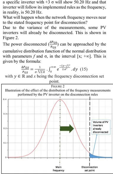
We have to be very clear about the interpretation of this. When the main frequency is f=50.1667 Hz, the display of

a specific inverter with +3 σ will show 50.20 Hz and that inverter will follow its implemented rules as the frequency, in reality, is 50.20 Hz.

What will happen when the network frequency moves near to the stated frequency point for disconnection?

Due to the variance of the measurements, some PV inverters will already be disconnected. This is shown in Figure 2.

The power disconnected (∆ ) can be approached by the cumulative distribution function of the normal distribution with parameters f and σ, in the interval [x; +∞]. This is given by the formula:

∆ =

. √ . .

( )²

. ² . (15)

with ∈ and x being the frequency disconnection set

point.

SECTION V: RESULTS

For the first scenario (common disconnection mode), the required primary reserve is 2150 MW.

When we simulate the second scenario (see the evolution of frequency in figure 3), we came to the value of 300MW, which is almost an order of magnitude less. As a result, the progressive disconnection of PV inverter is virtually sufficient to stabilize the frequency.

SECTION VI: CONCLUSION AND FURTHER

WORKS

These results show that the variance of the frequency measurements performed by hundreds of thousands of devices have an important influence on the system response. If we take this effect into account, the distribution grid is resilient to this issue.

This paper calls for three different types of future works. The first work to be performed is to review the different assumption and, mainly assumption 8, and carry out new studies with these new sets of assumptions.

FIGURE 2

Illustration of the effect of the distribution of the frequency measurements performed by the PV inverter on the disconnection rules

The second task consists of verifying these assumptions of the standard deviation of the frequency measurement by testing real inverters coming from the field. For Belgium, these have to have been in service prior to 2012.

Finally, it may be interesting to use a similar approach to the one developed in this paper to assess, in addition, the impact of accuracy of power measurements taken at the generation level on the system. For instance, it is described in the new European standards and requirements for generators (RfG) that, let us say at 50.2 Hz, an output power drop needs to be activated. This drop is an active power frequency response, decreasing the output power. However, this drop in function needs a local measurement of the output power and, from there, the question of impact of the dispersion of the power measurements on the system dynamics can also be applied.

REFERENCES

[1] ENTSO-E, P1: Load-Frequency Control and Performance, 2009.

[2] P. Anderson and M. Mirheydar, "A Low-Order System Frequency Response Model," IEEE

TRANSACTIONS ON POWER SYSTEMS, vol. 5, no. 3, p. 720, 1990.

[3] C. C. Arteaga, Optimisation of power system security with high share of variable renewables: consideration ofthe primary reserve deployment dynamics on a Frequency Constrained Unit Commitment model, Paris: Univertité Paris-Saclay, 2016.

[4] ELIA System Operator, "Ancillary services," 2016. [Online]. Available: http://www.elia.be/en/products-and-services/ancillary-services#anchorb1. [Accessed 20 08 2016].

[5] J. Bömer, K. Burges, P. Zolotarev, J. Lehner, P. Wajant, M. Fürst, R. Brohm and T. Kumm, "Frequency Stability Challenge," in 1st international Workshop on

Integration of Solar into Power Systems,

Aarhus/Danmark, 2011.

[6] CENELEC TS 50549-1 and TS 50549-2, Requirements for the connection of generators above 16 A per phase, 2016..

[7] IEEE, IEEE 929-2000 Recommended Practice for

Utility Interface of Photovoltaic (PV) Systems, Albuquerque, New Mexico, (United States of America): IEEE, 2000

APPENDIX I: TABLE 1

APPENDIX II: COUNTRIES IN SACE

Austria, Belgium, Bosnia and Herzegovina, Bulgaria, Croatia, Czech Republic, Denmark (western part), France, Germany, Greece, Hungary, Italy, Luxembourg, Macedonia (FYROM), Montenegro, the Netherlands, Poland, Portugal, Romania, Serbia, Slovakia, Slovenia, Spain, and Switzerland

APPRENDIX III: EULER APPROACH

To simulate the response of the system (also used in [2], and [3]) we the Euler's method. It is one of the simplest integration methods to compute the solution of a set of differential equations.

Let : → and ley us denote by :

→

( )

= , ( ) , ( ) =

We assume that we want to compute the evolution of z on the time interval , , where corresponds to the initial time and the final time.

To compute the value of z on this interval, the Euler method discretizes the function z into M constant pieces covering each of them a time step of length∆ . This method computes the value of z for m+1th time step based its value on the previous one, using the following equation:

= + ∆ . ( , ) ∀ = 1 … − 1 (6)

FIGURE 3

Evolution of frequency for scenario 1 and 2

TABLE1

Definition and Frequency Performance target

Reference Subject Value

f0 Nominal Frequency 50Hz F Actual frequency

∆ Frequency deviation: difference between actual

frequency and nominal frequency (f-f0)

∆ Activation of primary control +/- 20 _mHz

∆ , Full Activation of primary control reserves +/- 200 _mHz

∆ ,

Maximum permissible frequency deviation in steady-state (steady state = actual frequency after 30 s)

+/- 180 mHz

∆ , Maximum permissible frequency deviation _dynamic +/- 800 _mHz

RoCoF

Max Maximum Rate of Change of Frequency 2 Hz/s RoCoF 30s Rate of Change of Frequency after 30 seconds 0 Hz/s

By using this integration method in the context of equation (5) that we had to solve in this paper, we obtain the following specific recursive equation:

= + ∆ . 0 2 2. ∑₌₁ . _, . . , =1 − , =1 (A.III.1)