Requests for reprints should be sent to Christian Monseur, Université de Liège, FAPSE, Department Education, Bld. du Rectorat, 5 (B32) 4000 Liège, Belgium, e-mail: cmonseur@ulg.ac.be.
The Computation of Equating Errors
in International Surveys in Education
Christian Monseur University of Liège, Belgium
Australian Council for Educational Research, Australia Alla Berezner
Australian Council for Educational Research, Australia
Since the IEA’s Third International Mathematics and Science Study, one of the major objectives of interna-tional surveys in education has been to report trends in achievement. The names of the two current IEA surveys reflect this growing interest: Trends in International Mathematics and Science Study (TIMSS) and Progress in International Reading Literacy Study (PIRLS). Similarly a central concern of the OECD’s PISA is with trends in outcomes over time. To facilitate trend analyses these studies link their tests using common item equating in conjunction with item response modelling methods.
IEA and PISA policies differ in terms of reporting the error associated with trends. In IEA surveys, the standard errors of the trend estimates do not include the uncertainty associated with the linking step while PISA does include a linking error component in the standard errors of trend estimates. In other words, PISA implicitly acknowledges that trend estimates partly depend on the selected common items, while the IEA’s surveys do not recognise this source of error.
Failing to recognise the linking error leads to an underestimation of the standard errors and thus increases the Type I error rate, thereby resulting in reporting of significant changes in achievement when in fact these are not significant. The growing interest of policy makers in trend indicators and the impact of the evaluation of educational reforms appear to be incompatible with such underestimation.
However, the procedure implemented by PISA raises a few issues about the underlying assumptions for the computation of the equating error.
After a brief introduction, this paper will describe the procedure PISA implemented to compute the linking error. The underlying assumptions of this procedure will then be discussed. Finally an alternative method based on replication techniques will be presented, based on a simulation study and then applied to the PISA 2000 data.
Introduction
Policy-makers’ interest in the monitoring of educational systems and in the assessment of the effects of educational reforms have contributed to an increasing emphasis on trend indicators in the design of recent education surveys. Trends over time can inform policy-makers on how the achievement level of students in their country change in comparison with other countries, but also how within-country differences, such as the gender gap in achievement, evolve over time. The move to an emphasis on trend indicators represents a major challenge for achievement surveys.
Nowadays, TIMSS, PIRLS and PISA sur-veys are reporting trends in achievement on a regular basis (see Beaton et al., 1996a; Beaton et al., 1996b; Mullis et al., 2000; Martin et al., 2000; Mullis et al., 2004; Martin et al., 2004; Martin et al., 2003; OECD, 2004).
The IEA and PISA however differ in the way the standard error on trends in achievement is estimated. The standard error on trend estimates for IEA studies is based on the standard errors associated with the two independent population parameter estimates. This reported standard error, therefore, consists of the two sampling variances and the two measurement error variances.1 In the
PISA surveys, the standard error of the trend es-timates include a third error component, denoted as linking error (for a detailed description, see the PISA 2003 Technical Report, OECD, 2005) and discussed later.
This third component in the standard error reflects the variability of the trend estimates due to the selection of common-items. Indeed, under Rasch scaling assumptions, the same equating function would be obtained regardless of which common items are used because item-specific properties would be fully accounted for by the item’s Rasch estimated parameters. However, model mis-specifications always occur: small changes in the items, position effects, and cur-riculum effects can each effect modelled item 1 As student performance estimates are reported through plausible values, this measurement variance corresponds to the imputation variance.
behavior. Therefore, alternative sets of com-mon-items would generate differing equating transformations, even with very large examinee samples.
As stated by Sheehan and Mislevy (1988, p. 2), “it is standard practice to ignore the un-certainty associated with the linking step when drawing inferences that involve items from differ-ent subtests, a situation that arises, for example, in the measurement of change.” In a study using NAEP data, Sheehan and Mislevy (1988) applied a Jackknife approximation (Wolter, 1985, Rust and Rao, 1996) for quantifying the uncertainty of the link. These authors concluded that: “Whereas the size of the standard errors increased by only about 2 percent for estimates of change of indi-viduals, the increase in standard errors for groups is about 200 percent […] The component due to linking represents approximately 90 percent of the total error variance, on average” (Sheehan and Mislevy, 1988, pp. 18-19). Michaelides and Haertel (2004, pp. 24-25) observe similar results by comparing an analytical solution with a Boot-strap method: “The uncertainty in the accuracy of the mean due to sampling and measurement error […] is very small with large samples of examinees, and estimates of mean scores tend to have high precision with large samples. Hence, the equating errors, and in particular the error due to common-item sampling, appear larger relative to the standard error of the mean. Common-item sampling error constitutes 82.6 percent of the total variance, a lot larger than the other sources of error, which are affected by the sample size.”
As mentioned by these authors, this third component can be quite substantial. Not including a linking error will lead to a substantial under-estimation of the standard error. In their study, Sheehan and Mislevy (1988, p. 19) note that “the decrease in the mean reading proficiency of 9 year olds is approximately three standard errors when the uncertainty of the linking procedure is not account for, but only one standard error when it is.” In other words, an increase or a decrease of achievement will be reported as significant when in fact it is not significant and thus leading to an increase of Type I error.
TIMSS is currently the only survey with more than 2 time point estimates (i.e., 1995, 1999 and 2003). The TIMSS/REPEAT study (Martin et al., 2000; Mullis et al., 2000) reported at grade 8 four significant changes in mathematic achieve-ment: Latvia (+17), Canada (+10), Cyprus (+9) and the Czech Republic (–26). Unfortunately, Canada and the Czech Republic did not par-ticipate in the 2003 TIMSS survey. For the two remaining countries with a significant change between 1995 and 1999, Latvia obtained a mean estimate equal to the 1999 mean estimate. How-ever, Cyprus significantly decreased by 17 points (Mullis et al., 2004). In other words, IEA firstly reported a significant increase and then 4 years later, reported a significant decrease. It should be noted that out of about 20 countries with three time point estimates, Cyprus is the only case with such a profile. This result might reflect a real evolution of the student performance, or some unknown contextual effects during the data collection such as a strike but it could also be due to the selection of the anchor items. Failure to include the linking error increases the risk of such unexplained pattern that might, in the longer term, jeopardize the credibility for policy makers of trend indicators.
Now that the importance of the linking error has been presented, this paper will discuss the OECD method for computing the linking error, and will propose an alternative to the current OECD method. Concretely, this paper consists of four main sections:
(i) The OECD/PISA 2003 method for comput-ing the equatcomput-ing error will be described; (ii) The underlying assumptions of the OECD/
PISA 2003 program for computing such error will be listed and discussed; i.e., the stochastic independence of items, the item population, the response categories of items, the uniformity of the linking error;
(iii) An alternative method based on replication will be described and its efficiency tested through a simulation;
(iv) This replication method will be applied to the PISA 2003 reading assessment data.
The Anchoring Procedure
This section describes the procedure usu-ally implemented in international surveys in education for reporting the cognitive data on an existing scale. We will use the PISA survey as an example.
Reading literacy was the major domain in PISA 2000 while in PISA 2003 it was a minor domain. To link the two studies, a total of 28 of the 138 items used for the 2000 main assessment were used for the PISA 2003 assessment. These link items were used to report the 2003 reading literacy data on the 2000 reading literacy scale.
The steps for reporting the PISA 2003 read-ing literacy data on the 2000 combined readread-ing literacy scale were as follows (OECD, 2005): 1. Calibration of the 2003 reading literacy data
to get the PISA 2003 item parameters, i.e., the relative difficulty of the items on the Rasch scale;
2. Based on these item parameters, generation of the plausible values for reading literacy on the PISA 2003 data (for more informa-tion on plausible values, see for instance Wu, 2005);
3. Based on the item parameters from step 1, but only on the link items, generation of plausible values for reading literacy on the PISA 2000 data. By this time, two sets of plausible values are available for PISA 2000: (i) the original set of plausible values included in the PISA 2000 database and (ii) the set of plausible val-ues based on the PISA 2003 item parameters. Unfortunately, the mean and the standard deviation of the new set of plausible values will slightly differ from the PISA 2000 origi-nal plausible values. These differences reflect the changes in the difficulty of the link items between 2000 and 2003.
4. The linear transformation that will guarantee that the mean and the standard deviation of the new set of plausible values on the PISA 2000 data have a mean of 500 and a standard deviation of 100 is then estimated. This linear transformation can be written as:
PVcal_2000= +α βPVcal_2003, with β =σ σ cal cal _ _ 2000 2003 ,
and α=µcal_2000−βµcal_2003.
In the example, β = (100 / 110) = 0.909 and α = (500 – (0.909 × 505)) = 40.955.
5. This linear transformation is applied to the PISA 2003 plausible values, which guaran-tees that the student performance in 2003 is comparable to the student performance in 2000.
As stated earlier, with another set of link items the estimated linear transformation would have been different. As a consequence, there is an uncertainty in the transformation due to sampling of the link items.
Computation of the linking error for the PISA 2000-2003 Trend Indicators
in Reading
For each link item, we have two item param-eter estimates that are now on the same metric: (i) the 2000 item parameter estimate and (ii) the 2003 item parameter estimate. Both sets of items parameters are centred and then compared. Some of these link items show an increase in their rela-tive difficulty, others show a decrease. This means that some items seem relatively more difficult in 2003 than they were in 2000 and vice versa.
In PISA 2003 (OECD, 2005) the linking error was computed using the following formula:
σlink σ n
= 2 , (1)
where s2 is the variance of the item parameter
dif-ferences, and n is the number of link items used. This formula is consistent with the Michaelides and Haertel (2004, pp. 1-2) conclusions, i.e., “er-ror due to the common-item sampling does not depend on the size of the examinee sample, it is affected by the number of common items used.”
Let us consider that the item parameters from the 2003 calibration perfectly match the item parameters from the 2000 calibration. In other
words, the relative difficulty of the link items has not changed. In this particular case, all the differ-ences between the relative difficulty in 2000 and in 2003 would be equal to zero, and therefore the linking error would be equal to zero.
As the differences in the item parameters increase, the variance of these differences will increase and consequently the linking error will also increase. It makes sense for the uncertainty around the trend to be proportional to the changes in the item parameters.
Also, the uncertainty around the trend indi-cators is inversely proportional to the number of link items. From a theoretical point of view, only one item is needed. When the trend depends on a single item, the uncertainty will likely be large, but not estimable. As the number of link items increases, the uncertainty will decrease.
Table 1 provides the centred item parameter estimates for the reading literacy link items for PISA 2000 and PISA 2003, as well as the differ-ence between the two estimates for each item.
The variance of the difference is equal to 0.047486. The linking error is therefore equal to σlink σ n = 2 = 0 047486= 28 0 041 . . . (2)
On the PISA reading literacy scale, which has a mean of 500 and a standard deviation of 100, 0.041 corresponds to 3.75 score points. More information on the linking error is provided in the PISA 2003 Technical Report (OECD, 2005).
Assumptions behind the computation of the linking error
Equation (1) is similar to the formulae used for the computation of the standard error of a mean for a simple random sample from an infinite population (Cochran, 1977). However, two major issues need to be raised with regard to the use of this formula in the context of linking errors: the stochastic independence of the sampled units, and the status of the infinite population assumption.
Additionally, the use of linking error raises three further potential issues: the effect of partial credit items; the assumption that the linking
er-ror is a constant across countries; and national mis-specifications.
Stochastic Independence
Equation (1) is correct under the assump-tion that the estimates of the difference in item parameters that are provided by each item are independent. In practice, however, this assump-tion is unlikely to hold. One reason for this is that in PISA 2000 and PISA 2003, the reading literacy items are clustered in units (Adams and Wu, 2002; OECD, 2005). For instance, the 138 PISA 2000 reading literacy items were clustered into 37 units that each relied on a common stimu-lus; when link items were chosen, they had to be selected together with the other items that made up whole units.
Adapting a formula from Kish (1965), the sampling variance of the mean difference for a cluster sample of items is equal to:
σlink σB σ B W B W n n n 2 = 2+ 2 , (3)
for infinite populations, with sB2 the between
cluster variance, sW2 the within cluster variance,
nB the number of sampled clusters and nW the number of units sampled per cluster—which is assumed to be common to all clusters.
The between and within cluster variances of the difference in item parameters between 2000 and 2003 can be estimated by an ANOVA analysis.
Table 1
Item parameter estimates in 2000 and 2003 for the Reading link items
Centered Parameter Centered Parameter
Item Name estimate in 2003 estimate in 2000 Difference
R055Q01 –1.28 –1.347 –0.072 R055Q02 0.63 0.526 –0.101 R055Q03 0.27 0.097 –0.175 R055Q05 –0.69 –0.847 –0.154 R067Q01 –2.08 –1.696 0.388 R067Q04 0.25 0.546 0.292 R067Q05 –0.18 0.212 0.394 R102Q04A 1.53 1.236 –0.290 R102Q05 0.87 0.935 0.067 R102Q07 –1.42 –1.536 –0.116 R104Q01 –1.47 –1.205 0.268 R104Q02 1.44 1.135 –0.306 R104Q05 2.17 1.905 –0.267 R111Q01 –0.19 –0.023 0.164 R111Q02B 1.54 1.395 –0.147 R111Q06B 0.89 0.838 –0.051 R219Q01T –0.59 –0.520 0.069 R219Q01E 0.10 0.308 0.210 R219Q02 –1.13 –0.887 0.243 R220Q01 0.86 0.815 –0.041 R220Q02B –0.14 –0.114 0.027 R220Q04 –0.10 0.193 0.297 R220Q05 –1.39 –1.569 –0.184 R220Q06 –0.34 –0.142 0.196 R227Q01 0.40 0.226 –0.170 R227Q02T 0.16 0.075 –0.086 R227Q03 0.46 0.325 –0.132 R227Q06 –0.56 –0.886 –0.327
The Total mean square is an unbiased esti-mate of the total variance, as the error (or within cluster) mean square is an unbiased estimate of the error variance.
An unbiased estimate of the between cluster variance can be obtained by:
σB MSB MSW n 2 0 1076 0 0264 28 8 0 0812 3 5 0 0232 = − = − = = . . ( / ) . . . .
As shown in Table 2 the between cluster variance in the item parameter shifts is as large as the within cluster variance.
According to formulae (3), an estimate of the linking error is:
σlink σB σ B W B W n n n = + = + = 2 2 0 0232 8 0 0264 28 0 062 . . . ,
which indicates that the linking error reported in the PISA 2003 Technical Report (OECD, 2005) is underestimated due to the embedded structure of items within units.
The Item Population
Each of the above formulae assumes that the trends have been estimated using a sample of items from an infinitely large pool. We now consider the linking error when all items are used as common-items. In 2001, the IEA conducted the Reading Literacy Repeat Study (Martin et al., 2003) and nine countries that participated in the IEA/Reading Literacy Study in 1991 re-adminis-tered the 1991 test without adding or removing any item. Similarly, PISA 2006 used all reading
items from PISA 2003. In these circumstances, does it make sense to include the uncertainty due to common-item sampling as, in fact, all items are used as common-items? In other words, should the item pool from which common items are se-lected be considered as a finite existing population or as a simple random sample of a hypothetical infinite population?
Equation (1) gives an estimate of the sam-pling variance of a mean under the assumption of a simple random sample from an infinite tion. Considering the item pool as a finite popula-tion would require replacing formulae (1.1) by:
− − = 1 2 2 ) ˆ ( sn NN n sµ (4)
where N represents the size of the item pool and
n the number of common-items. In the case of
the IEA Reading Literacy study, as all 1991 items were used as common-items in 2001, N=n and therefore, as the exhaustivity coefficient
N n N − − 1
would be equal to 0, the linking error would also be equal to 0. In the case of PISA 2003, the ex-haustivity coefficient would be equal to
138 28 138 1 0 80292 − − = . .
This means that the application of this finite population correction would reduce the standard error by a factor of 0.896.
According to Michaelides and Haertel (2004, p. 6), “common items are chosen from a hypothetical infinite pool of potential items.” Cronbach, Linn, Brennan, and Haertel (1997) also support this point of view. A test score is based on an examinee’s performance on a particular test form consisting of certain items. What is of most interest is not how well the examinee did on those particular items at that particular occasion. Rather it is the inference drawn from that example of performance to what the examinee could do across many other tasks requiring the application of the same skills and knowledge.
Table 2
ANOVA table of the link item difference in Reading
SS DF MS
Between 0.7532 7 0.1076
Within 0.5288 20 0.0264
By extension, we can consider that common items are selected from a hypothetical infinite population, and therefore no correction for sampling fraction should be applied. Following this line of argument, a linking error should also be included in the trend estimate standard error when comparing the PISA 2003 reading perfor-mance with the PISA 2006 reading perforperfor-mance or the 1991 IEA/Reading Literacy with the 2001 results.
Polytomous versus dichotomous items
Out of the 28 common reading items from the 2000 and 2003 data collections for PISA, six are polytomous items. As shown in Table 1, the linking error is based on the variance of the difference in item difficulty estimates. The PISA linking errors do not integrate a possible change in the category item parameters. Further, by representing the polytomous items by their overall difficulties, the reported linking errors under-represents their contributions in the equat-ing transformation.
Uniformity of the linking error
Monseur, Sibberns and Hastedt (2007), by reanalyzing the IEA/Reading Literacy Repeat
study, found that the equating errors were
sub-stantially different from one country to another. Further, they observed a high correlation between the absolute value of the trends and the size of the linking error. However, these correlation coef-ficients are based on only eight countries.
These different results suggest that a linking error should be computed by country and not, as it was done in PISA 2003, at the international level only.
National mis-specification
In PISA 2003, as it is also expected in any in-ternational survey, the shift in the item parameters between two data collections also varies from one country to another. Therefore, the impact of removing a unit (that is, a related set of test items) on the country mean estimate in 2003 can differ between countries.
The Jackknife replication method for the computation of the linking error:
A simulation study
As stated by Rust and Rao (1996, p. 285), “replication methods are often referred as resa-mpling techniques. The common principle that these methods have is to use computational inten-sity to overcome difficulties and inconveniences in utilizing an analytic solution to the problem at hand. Briefly, the replication approach consists of estimating the variance of a population parameter of interest by using a large number of somewhat different subsamples (or somewhat different sampling weights) to calculate the parameter of interest. The variability among the resulting esti-mates is used to estimate the true sampling error of the initial, or full-sample, estimate.”
The adaptation of resampling techniques in the context of the linking error would imply computing the trend estimates in achievement on subtests by removing each time an item or a set of items and using the variability of these trend estimates to estimate the linking error. Specifi-cally, the Jackknife replication method requires removing an item for each replicate in the case of a test with only independent items, or a unit for each replicate in the case of embedded structures of items like the PISA test. Therefore, if a test consists of 30 independent items, the Jackknife method will compute 30 replicates each of them based on 29 items. If a test consists of 10 stimuli (like a text in a reading test), with several items related to each stimulus, the Jackknife method will compute 10 replicates, each of them based on 9 texts with their respective items.
To evaluate the accuracy of a Jackknife procedure for estimating the linking error, several simulations were conducted.
For avoiding the contamination of the sam-pling variance, a single population of 10 000 students was used at two different times, denoted T1 and T2. The latent proficiency of these 10 000 students is normally distributed with a mean of zero and a standard deviation of one.
In T1, 50 items with a true item difficulty randomly drawn from N(0,1) are “administered.”
The probability of each student succeeding on each of the 50 items is then computed according to the Rasch model, i.e.,
P Xij j i j i j ( , ) exp( ) exp( ). = = − + − 1 1 |β δi β δ β δ
This probability is then compared to a uni-form distribution. If the probability of succeeding on the item is larger than the uniform distribu-tion value, the student is considered as having succeeded on the item, otherwise, the student is considered as having failed the item. The data matrix is then submitted to ACER ConQuest (Wu, Adams and Wilson, 1997) and plausible values are generated.
At T2, the 50 items are allocated to 10 units: item one to item five constitute unit one, item six to item ten constitute unit two and so on. Shifts in the original true item difficulty are then introduced at the unit level and at the item level. The combined shift is normally distributed with a mean of zero and a standard deviation of 0.5. Three decompositions of the combined variance into the unit and the item levels were implemented:
(i) 25 percent at the unit level and 75 percent at the item level;
(ii) 50 percent at the unit level and 50 percent at the item level; and,
(iii) 75 percent at the unit level and 25 percent at the item level.
The estimation of the trends requires: (i) the scaling of the population at T1 with the
items of T1, i.e., before the introduction of the item difficulty shift;
(ii) the scaling of the population at T2 with the items of T2, i.e., after the introduction of the item difficulty shift; and,
(iii) the scaling of the population at T1 with the item difficulties anchored at their value as computed in T2.
For each variance decomposition type, 100 possible tests were generated, i.e., 100 different shifts were added to the original true item pa-rameters. These 100 trend estimates will then be used later to empirically build the linking error distribution.
To study the accuracy of the Jackknife esti-mate of the linking error, it is required, for each possible test, to estimate a linking error. If the Jackknife procedure is appropriate in the context of estimating the linking error, then the average of the Jackknife estimates of the linking error should be identical to the standard distribution of the empirical linking error distribution.
Therefore, ten subsets of nine units are created per possible test and for each subtest, the linking procedure described above is imple-mented on the whole test. For each possible test, there is a trend estimate on the whole test and there are ten trend estimates each based on one of the ten subtests.
The estimator of the linking error is: 2 1 () ) ˆ ( (ˆ ˆ) ) 1 ( θ θ sθ = −
∑
− = G i i G G , (5)where θˆ represents the trend estimate on the whole set of items, θi represents the trend estimate
on one of the ten subsets of items and G the num-ber of replicates, i.e., the ten in the simulation:
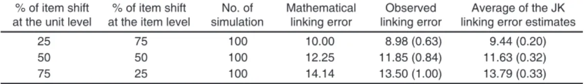
Table 3 provides the results of these simu-lations for each variance decomposition of the item shift.
The expected linking error for the third vari-ance decomposition, i.e., 75% at the unit level and 25% at the item level, is equal to:
Table 3
Analytical, empirical and JK linking error estimates
% of item shift % of item shift No. of Mathematical Observed Average of the JK at the unit level at the item level simulation linking error linking error linking error estimates
25 75 100 10.00 8.98 (0.63) 9.44 (0.20)
50 50 100 12.25 11.85 (0.84) 11.63 (0.32)
σlink σB σ B W B W n n n = + = + = 2 2 100 0 75 0 50 10 0 25 0 50 50 100 ( . )( . ²) ( . )( . ²) 114 14. .
The observed linking error corresponds to the standard deviation of the 100 trend estimates computed on the whole test. The last column corresponds to the mean of the 100 Jackknife standard errors.
As shown by Table 3, the Jackknife estimates of the linking error are very close to the observed linking error estimates and to the mathematical solutions, as computed by equation (3). It should however be noted that the Jackknife estimate significantly differs from the analytical solution for the first variance decomposition (25 percent at the unit level and 75 percent at the item level) and is close to being significantly different for the second decomposition (50 percent at the unit level and 50 percent at the item level). In both cases, the Jackknife estimates tend to be lower than the analytic solution.
Further simulations should be conducted for analyzing the accuracy of the Jackknife es-timations of the linking error, depending on the number of items and on the combined standard deviation of the item parameter shifts. However, these preliminary results confirm that the Jack-knife technique can be considered as a promising method for computing the linking error.
Application of The Jackknife replication method for the computation of the linking
error: PISA 2000 and PISA 2003
As mentioned earlier, the replication tech-niques are of particular interest when no analytical solution exists or when this analytical solution is highly complex. Recall that the simulation involves only one data set and therefore the item parameter estimates at time one perfectly fit the data. In the context of international surveys in education, the item calibration is based on an international calibration sample with an equal number of observations per country. Then student performance estimates are generated for each
country, based on the entire national samples. The international item calibration is not necessarily the most appropriate calibration for a particular country as national and cultural differences in the curriculum might change the relative difficulty of some items. The differences in the item parameter estimates between the national and international calibration, usually denoted as Item-by-Country
Interaction, are an additional source of error that
affect the trend estimates. For instance, if an item presents a large difference between the national item difficulty estimate and the international item difficulty, removing that item will have a larger impact for that particular country than removing an item that presents no item by country interac-tion. Applying a Jackknife method for estimating the linking error in this context will therefore reflect these national mis-specifications and the uncertainty of the international linking step.
The Jackknife method of estimating the linking error has been applied to the PISA data-bases. The same steps as described in the previ-ous section were applied. Briefly, it consists of replicating the steps described above on the eight subsets of seven reading units. The first replica-tion is based on unit two to unit eight, the second replication is based on unit one, units three to eight and so on.
Table 1 in the appendix and Figure 1 follow-ing provide the shift in the country mean estimate of the combined reading scale for PISA 2003 in comparison with the mean estimates computed on the whole set of reading anchor items. For instance, removing unit one from the set of anchor items would have raised the mean estimate of Australia in 2003 by 1.82 points. Removing unit six would have decreased the results of Australia by 6.17 points on the PISA scale.
At the OECD level, removing unit one would have raised the OECD mean estimate by 4.14 and removing unit two would have decreased the OECD mean by 3.96 points. These changes in the OECD mean estimates in reading are con-sistent with the item parameter shifts presented in Table 1.
Some countries present large shifts in some replications. These shifts are also consistent with
Table 4
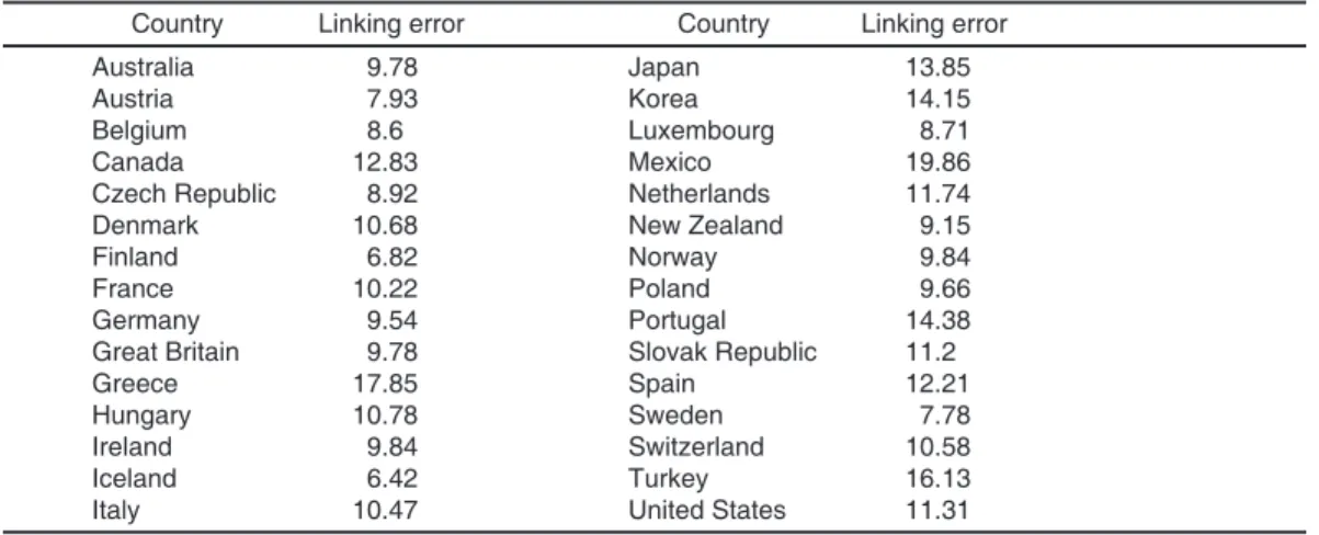
Linking error estimate by country
Country Linking error Country Linking error
Australia 9.78 Japan 13.85 Austria 7.93 Korea 14.15 Belgium 8.6 Luxembourg 8.71 Canada 12.83 Mexico 19.86 Czech Republic 8.92 Netherlands 11.74 Denmark 10.68 New Zealand 9.15 Finland 6.82 Norway 9.84 France 10.22 Poland 9.66 Germany 9.54 Portugal 14.38 Great Britain 9.78 Slovak Republic 11.2 Greece 17.85 Spain 12.21 Hungary 10.78 Sweden 7.78 Ireland 9.84 Switzerland 10.58 Iceland 6.42 Turkey 16.13 Italy 10.47 United States 11.31
Figure 1. Shift in the country mean estimate on the reading scale if one reading unit is removed from the set of 8 anchoring units -20 -15 -10 -5 0 5 10 15 United States Turkey Sw itzerland Sw eden Spain Slovak Republic Portugal Poland Norw ay New Zealand Netherlands Mexico Luxembourg Korea Japan Italy Ireland Iceland Hungary Greece Great Britain Germany France Finland Denmark Czech Republic Canada Belgium Austria Australia OECD Mean
the national item parameters. For instance, the in-ternational item parameters for the three items in unit six are respectively –0.520, 0.308 and –0.887. For Australia, these are respectively –0.470, –1.243 and –1.772. The second item of unit six has an item by country interaction of 1.5 logits and the last one of about one logit. On average, the national item parameters for unit two in Greece are lower by one logit than the international item parameters. The impact of removing that unit is equal to 15.79 score points for Greece.
Table 4 presents the linking error estimated with the Jackknife replication method. These linking error estimates are substantially higher than those obtained from the estimation method used in PISA 2003. The differences between the Jackknife estimates of the linking error and the PISA 2003 ones are due to several factors: (i) the embedded structure of the PISA items
within units;
(ii) the partial credit items;
(iii) the national mis-specifications or the so-called item-by-country interactions.
With a mean estimate in reading equal to 522 in PISA 2000 and to 498 in PISA 2003, Japan presents the largest decrease in reading literacy. This difference has been reported as highly sig-nificant in the PISA 2003 initial report. With the linking error estimated by the Jackknife method, this difference would no longer be considered as significant.
Conclusions
By reporting an equating error that needs, in some circumstances, to be added to the sampling and imputation variance, PISA has added an important innovation to large-scale assessments. However, this paper raises four issues that might require further investigation before reporting an equating error in future PISA cycles. These issues are:
1. the hierarchical structure of the PISA items;
2. finite versus infinite populations;
3. polytomous items; and
4. uniformity of the equating error.
Replication methods (Jackknife or Boot-strap) seem to offer an interesting alternative to the analytical solution that can easily deal with the hierarchical structure of the PISA items. The results of the simulation are quite promising.
The variability of the equating error would require the computation of specific equating errors for each country. This also presents the advantage of integrating particular country model mis-specifications in the computation of the equating error, even though it does not solve the problem for subnational comparisons.
This paper also raises the importance of the number of anchoring items, especially in a design with items embedded in units. Increasing the number of items will decrease the effect of national mis-specifications.
References
Adams, R. J., and Wu, M. (Eds.) (2002). PISA
2000 technical report. Paris: OECD
Publica-tions.
Beaton, A. E., Mullis, I. V. S., Martin, M. O., Gonzalez, E. J., Kelly, D. L., and Smith, T. A. (1996a). Mathematics achievement in the
middle school years: IEA’s third international mathematics and science study. Chestnut Hill,
MA: Boston College.
Beaton, A. E., Martin, M. O., Mullis, I. V. S., Gonzalez, E. J., Smith, T. A., and Kelly, D. L. (1996b). Science achievement in the middle
school years: IEA’s third international math-ematics and science study. Chestnut Hill, MA:
Boston College.
Cochran, W. G. (1977). Sampling techniques. New York: Wiley and Sons.
Cronbach, L. J., Linn, R. L., Brennan, R. L., and Haertel, E. H. (1997). Generalizability analysis for performance assessments of stu-dent achievement or school effectiveness.
Educational and Psychological Measurement, 57, 373-399.
Dagnelie, P. (1998). Statistique théorique et
appliquée. Tome 1: Statistique descriptive et bases de l’inférence statistique. Paris and
Bruxelles: De Boek and Larcier.
Harris, D. J., and Crouse, J. D. (1993). A study of criteria used in equating. Applied
Measure-ment in Education, 6, 195-240.
Kish, L. (1995). Survey sampling. New York: Wiley and Sons.
Martin, M. O., Mullis, I. V. S., Gonzalez, E. J., Gregory, K. D., Smith, T. A., Chrostowski, S. J., et al. (2000). TIMSS 1999 international science
report. Chestnut Hill, MA: Boston College.
Martin, M. O., Mullis, I. V. S., Gonzalez, E. J., and Kennedy, A. M. (2003). PIRLS trends
in children’s reading literacy achievement 1991-2001. IEA’s repeat in nine countries of the 1991 reading literacy study. Chestnut Hill,
MA: Boston College.
Martin, M. O., Mullis, I. V. S., Gonzalez, E. J., and Chrostowki, S. K. (2004). TIMSS 2003
international science report: Findings from the IEAs trends in international mathematics and science study at the fourth and eighth grades.
Chestnut Hill, MA: Boston College.
Michaelides, M. P., and Haertel, E. H. (2004).
Sampling of common items: An unrecognized source of error in test equating (Technical
Report). Los Angeles: Center for the Study of Evaluation and National Center for Re-search on Evaluation, Standards, and Student Testing.
Monseur, C., Sibberns, H., and Hastedt, D. (2006, November). Equating errors in international
survey in education. IEA Second International
Research Conference, Washington, DC. Mullis, I. V. S., Martin, M. O., Gonzalez, E. J.,
Gregory, K. D., Garden, R. A., O’Connor, K. M., et al. (2000). TIMSS 1999 international
mathematics report. Chestnut Hill, MA:
Bos-ton College.
Mullis, I. V. S., Martin, M. O., Gonzalez, E. J., and Chrostowski, S. J. (2004). TIMSS 2003
in-ternational mathematics report: Findings from the IEAs trends in international mathematics and science study at the fourth and eighth grades. Chestnut Hill, MA: Boston College.
Rust, K. F., and Rao, J. N. K. (1996). Variance estimation for complex surveys using replica-tion technique. Statistical Methods in Medical
Research, 5, 283-310.
OECD (1999). Measuring student knowledge and
skills: A new framework for assessment. Paris:
OECD Publications.
OECD (2004). Learning for tomorrow’s world:
First results from PISA 2003. Paris: OECD
Publications.
OECD (2005). PISA 2003 technical report. Paris: OECD Publications.
Sheehan, K. M., and Mislevy, R. J. (1988).
Some consequences of the uncertainty in IRT linking procedures. (Report No:
ETS-RR-88-38-ONR) Princeton, NJ: Education Testing Service.
Wolter, K. M. (1985). Introduction to variance
estimation. New York: Springer-Verlag.
Wonnacott, T. H., and Wonnacott, R. J. (1991).
Statistique: économie-gestion-sciences-méde-cine. Paris: Economica.
Wright. B. D., and Stone, M. H. (1979). Best test
design. Chicago: MESA Press.
Wu, M. L., Adams, R. J., and Wilson, M. R. (1997). ConQuest: Multi-aspect test software [Computer program]. Camberwell: Australian Council for Educational Research.
Wu, M. (2005). The role of plausible values in large scale surveys. Studies in Educational
Appendix
Table 1
Shift in the country mean estimate on the reading scale if one reading unit is removed from the set of 8 anchoring units
Shift in the country mean without
Country Unit 1 Unit 2 Unit 3 Unit 4 Unit 5 Unit 6 Unit 7 Unit 8
Australia 1.82 –3.32 –1.09 4.07 –3.6 –6.17 4.3 2.77 Austria 3.34 –2.66 2.48 1.58 0.4 –4.17 –4.79 2.13 Belgium 6.79 –1.03 0.07 1.87 1.67 –0.53 –5.54 0.24 Canada –0.06 –6.64 1.41 3.87 –6.64 –5.31 3.32 6.62 Czech Republic 0.6 –3.31 –0.21 –0.93 0.37 2.82 –3.9 7.44 Denmark 6.52 6.31 –2.79 3.34 0.37 –3.11 –3.41 –2.76 Finland 1.87 1.36 –1.85 0.23 –0.13 –3.7 –5.05 2.24 France 3.06 3.01 2.3 2.71 –0.36 –6.11 –6.97 1.53 Germany 5.73 –0.79 1.07 4.39 1.77 –2.25 –6.24 –1.7 Great Britain 1.53 –2.82 –1.07 3.07 –1.42 –6.68 4.95 4.15 Greece 6.95 –15.79 1.37 6.16 –4.04 0.91 2.54 1.67 Hungary 9.04 –3.49 1.12 4.65 –1.06 –3.44 –1.62 –0.65 Iceland 3.86 –1.06 –2.07 1.34 3.94 –0.99 –2.89 0.31 Ireland 0.02 –4.48 –0.65 1.5 –3.52 –6.18 3.16 5.23 Italy 4.49 –8.77 1.68 3.39 3.17 1.33 –1.44 –0.3 Japan 9.76 1.13 –1.37 4.74 –7.72 –5.55 1.96 –2.03 Korea 6.43 –3.83 0.31 –0.93 –0.16 –2.53 12.42 –3.34 Luxembourg 2.95 –4.48 1.88 2.61 4.68 –2.2 –4.54 0.45 Mexico 5.1 –15.79 1.79 8.42 –4.23 1.92 0.09 8.93 Netherlands 7.3 3.68 –2.75 4.11 2.31 –3.13 –2.91 –6.52 New Zealand 1.88 –1.56 –0.84 3.9 –4.71 –5.43 1.83 4.32 Norway 6.75 0.33 –3.35 4.15 –1.91 –5.42 1.35 –1.25 Poland 0.65 –7.83 –4 3.14 0.26 0.7 –0.03 4.31 Portugal –0.84 –12.85 3.26 2.15 3.22 –0.76 –0.44 6.65 Slovak Republic –0.82 –5.48 2.54 –0.35 1.76 1.16 –4.92 8.8 Spain 4.33 –5.94 3.43 4.31 –5.13 –2.22 –1.77 7.17 Sweden 5.77 –1.21 0.24 2.97 –0.84 –4.66 –1.64 –0.65 Switzerland 5.6 –3.4 3.68 3.21 1.68 –2.21 –6.66 –3.05 Turkey 11.75 –11.26 3.75 0.05 –0.48 –1.13 –2.21 3.45 United States 2.07 –6.78 –0.45 4.61 –1.53 –5.18 4.29 5.19 OECD mean 4.14 –3.96 0.33 2.95 –0.73 –2.67 –0.89 2.04