HAL Id: hal-00451898
https://hal.archives-ouvertes.fr/hal-00451898
Submitted on 25 Jun 2019
HAL is a multi-disciplinary open access archive for the deposit and dissemination of sci-entific research documents, whether they are pub-lished or not. The documents may come from teaching and research institutions in France or abroad, or from public or private research centers.
L’archive ouverte pluridisciplinaire HAL, est destinée au dépôt et à la diffusion de documents scientifiques de niveau recherche, publiés ou non, émanant des établissements d’enseignement et de recherche français ou étrangers, des laboratoires publics ou privés.
Sébastien Briot, Anatol Pashkevich, Damien Chablat
To cite this version:
Sébastien Briot, Anatol Pashkevich, Damien Chablat. Optimal Technology-Oriented Design of Parallel Robots for High-Speed Machining Applications. the 2010 IEEE International Conference on Robotics and Automation (ICRA 2010), May 2010, Anchorage, United States. �hal-00451898�
Abstract— In this paper, a new methodology for the optimal design of parallel kinematic machine tools is proposed. This approach is based on the concept of the maximal inscribed parallelepiped and uses technology-oriented constraints that are motivated by particular applications. This methodology is applied on two translational parallel robots with three degrees-of-freedom (DOF): the Y-STAR and the UraneSX. An analysis of the size of their workspace as a function of the design constraints is made. It is shown that, for identical workspaces with similar properties, the size of the legs of the UraneSX are greater than for the Y-STAR, thus leading to larger deformations. However, the footprint surface needed in order to install the Y-STAR is about two times bigger than for the UraneSX. Therefore, it may be interested to use the UraneSX in order to save some place on ground in manufacturing centres.
I. INTRODUCTION1
arallel kinematic machines (PKM) are commonly claimed to offer several advantages over their serial counterparts, such as high structural rigidity, better payload-to-weight ratio, high dynamic capacities and high accuracy [1–3]. Therefore, they are prudently considered as promising alternatives for many modern material processing operations, especially in automotive and aerospace industry, in which high accuracy positioning and high-speed motions of a work tool are required. Thus, PKM have gained essential attention of a number of companies and researchers. However, most of the existing PKM still suffer from two major drawbacks, namely, a complex workspace and highly non-linear input/output relations [4, 5].
For most of PKM, the performances vary considerably for different points in the workspace and for different directions at one given point. This is a serious disadvantage for machining applications [6, 7], which require regular workspace shape and acceptable kinetostatic performances throughout. In milling applications, for instance, the machining conditions must remain constant along the whole tool path [8]. Nevertheless, in many research papers, this criterion is not taken into account in the algorithmic methods used for the optimization of robots [9, 10].
This work is focused on the optimal design of a robot for given geometric, kinematic and kinetostatic properties derived from technical applications (e.g. size of the workspace, maximum speeds, forces transmission, Manuscript received September 10, 2009.
S. Briot, A. Pashkevich and Damien Chablat are with the IRCCyN, Nantes, 44321 France (corresponding author: +33240376958; fax: +33240376930; e-mail: [email protected]).
S. Briot and A. Pashkevich are also with the Ecole des Mines, Nantes, 44307 France.
accuracy). The main contribution of this paper is in the area of application of the operation research methods to the integrated design optimization of complex mechanical structures, such as parallel robots. The proposed approach operates with the ‘workspace grid’ that is evaluated using a dedicated dynamic-programming-based algorithm allowing, for each particular set of the design parameters, to estimate the largest cuboid-shaped workspace with the desired properties. Further, the workspace parameters are evaluated in the frame of the global optimization. Finally, contrary to many works on optimal design of parallel robots (see for example [11, 12]), it is proposed in this paper to use technology oriented indices in order to define the optimal design parameters.
The paper will be divided as follows. In the second part, the design problem and methodologies are explained. In the third section, the performance measures used are presented. In part four, the optimization procedure is described and it is applied on an industrial case study in part five. Finally, in the last section, conclusions are drawn.
II. DESIGN PROBLEM AND METHODOLOGY
Manipulator design traditionally begins with the selection of a kinematic framework and achieving certain geometric goals such as workspace size and dexterity. Besides, for particular manufacturing tasks, the manipulator geometry is optimized with respect to the desired velocity, accuracy or force transmission factors. This yields a simplified CAD model of a relevant mechanism that defines basic dimensions of the links and spatial locations of all active and passive joints, as well as joint limits. At the next step, this model should be detailed by providing real shapes of links to produce the solid CAD model.
To formulate the design problem, let us define the manipulator geometry by the mapping g: W, where = 1 × … n and W = p1 × … pn denote respectively the
configuration space and the workspace. i are the joint
coordinates and pi are the coordinates of the end-effector. n
is the number of DOF. Besides, for each workspace point p W, let us define the matrices Kv(p, ), Kf(p, ), Ka(p, ),
that describe various mechanical properties of the manipulator (velocity, force transmission, accuracy, etc.) for any given set of the design parameters . Let us also assume that for each type of the matrices K, {v, f, a, …}, there
are defined physically consistent scalar measures (K),
{i, t, …} that may be directly included in the design objectives or constraints. Some examples of such measures (isotropy, transmission factors, etc.) are presented in the following sections.
Sébastien Briot, Anatol Pashkevich and Damien Chablat
Optimal Technology-Oriented Design of Parallel Robots for
High-Speed Machining Applications
us introduce the performance measures (g, ), {m, l,
w, …}, that depend both on the adopted geometrical structure g and the physical parameters of the links . Examples of the global measures include the total mass of the manipulator, the length of the principal links, the workspace size, etc.
Then, following the general methodology adopted for the considered application area (high-speed machining), the design optimisation problem can be stated as achieving the best value of the performance indices
( , )min,
π
π
g (1)
subject to the constraints
K(p,π) S, , (2)
that must be satisfied for all points of the cuboid workspace
W0 of size a × b × c, which includes the manufacturing task.
It should be noted that the latter assumption (concerning the workspace shape) is essential here and allows considerably speed-up the optimization routines. Since in practice this problem cannot be solved by the direct search methods, in the following subsections, there will be presented the discretisation scheme and relevant optimisation algorithms allowing to obtain desired solutions in reasonable time.
III. PERFORMANCE MEASURES
Let us present here the most essential technology-oriented performance measures that are used in the following of this paper. Traditionally, they are directly included in the design constraints/objectives to be satisfied or optimized throughout the prescribed workspace. However, in this paper, each performance measure is preliminary converted in an alternative form that defines the workspace subset where the relevant criterion is higher/lower of the desired value.
It should be noted that, in the following of this paper, our analysis will be restrained to 3-DOF translational PKM as they are mostly used for machining of materials.
A. Size of the workspace
Using the set of parameters , the workspace W may be generated using the kinematic equations and the joint limits [1].
Since, for the considered application, the desired regular workspace is a parallelepiped W0 of size {a0 × b0 × c0}, the
relevant measure may be defined by the largest similar object Wabc = {µa
0 × µb0 × µc0} inscribed in W, i.e.
T W W
T W T W 0 T 0 ( ); ( , ) argmax ( ) , abc (1)where µ, T are respectively the scalar scaling factor and the coordinate transformation operator in the Cartesian space. This notion is the fundamental issue of this paper and is discussed in details in the following section.
B. Velocity transmission factors
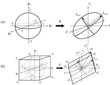
For quantifying the speed capability of a manipulator, several kinematic performance indices are defined using the Jacobian matrix J (see [13]), such as the condition number, the largest/smallest singular value (also called the maximal/
respectively – Fig. 1a), the dexterity, the manipulability, etc. However, as mentioned by Merlet in [13], the previously cited indices does not take into account the ‘technological reality’ of the mechanism, as they are based on the use of the Euclidian norm of the input velocity vector Φ (||Φ || being considered equal to 1) while it is clear that each actuator may have a velocity i [–imax,imax], where i and imax
are the actual and maximal velocities for the actuator i (i = 1 to n). Thus, it is necessary to redefine the transmission factors, of which expressions are presented in the next subsections.
1. Velocity transmission along all directions of the workspace.
Normalizing the problem and considering that max
i
= 1, i.e. replacing the unit sphere by a unit cube (Fig. 1b), one can obtain the image of the unit square by the transformation
f: x J x. The obtained figure is a parallelepiped, where point Bj is considered to be the image of point Aj by the
transformation f.
One can now define the minimal and maximal transmission factors min
v k and max v k . Factor max v k is the largest distance from the origin of the frame to the faces of the parallelepiped. Its corresponding expression may be written as: ) ) ( ( max max j j v k Jq e , for j = 1 to 4 (2) where e1 = [+1, +1, +1]T, e2 = [+1, –1, +1]T, e3 = [+1, +1, – 1]T and e 4 = [+1, –1, –1]T.
To obtain the expression of min
v
k , more computations are required. Indeed, min
v
k is the smallest distance between point O and the faces of the parallelepiped.
Let us consider that the Jacobian matrix J may be decomposed into three vectors I1, I2 and I3 such as:
I1 I2 I3
J . (3)
The faces of the parallelepiped are the images by the transformation f of the faces of the unit cube, i.e. there are attained when at least one actuator is at its maximal velocity
max
i
( max1
i
, i = 1, 2, 3). Therefore, the parameterized expressions of the faces of the parallelepiped are, for any vector = [1, 2]T, 1,2[1,1]:
( ) ( ) ( )
( ) ) ( m T m ijk m ijk m ijk m ijk x y z J1δ J2 V , (4) for m = 1 or 2, i, j, k = 1, 2, 3, i ≠ j, i ≠ k, j ≠ k, where ] [Ii Ij J1 , J2 (1)mIk. (5) The distances || (m) ijkV || (m = 1, 2) from the origin to any point belonging to the faces are given by
) ( ) ( ) ( m ijk T m ijk m ijk V V V . (6)
Finding the minimum of this expression remains to computing the minimum of || (m)
ijk
V ||². Thus, differentiating expression (6) with respect to the parameter , it may be found that the minimum appears when
(a)
(b)
Fig. 1. Mapping, using the Jacobian matrix, (a) of the unit sphere and (b) of the unit cube.
Tij ij
Tij k m ijk δ J J J J V δ 1 2 ) ( 0 . (7) Verifying that the components of belong to the interval [– 1, +1] and introducing them into (6), it may be found that: Vijkm
Vijkm
JT2J2
JT2J1 JT1J1 JT1J2
1 )
(
min min
(8) Thus, the expression of min
v k is ) ( min min , , , min ijkm m k j i v k V , (98) for m = 1, 2, i, j, k = 1, 2, 3, i ≠ j, i ≠ k, j ≠ k.
It should be mentioned that, if the components of do not belong to the interval [–1, +1], thus the obtained value for
min
ijkm
V does not correspond to the minimal distance between the face of the parallelepiped and the centre of the frame, but between the plane on which is lying the face under consideration and the centre of the frame. It could be proved that, even if this happens, the value of min
v
k will be obtained when considering another face for which the components of will belong to the interval [–1, +1]. Therefore, there is no need to use other expressions than those presented above. 2. Velocity transmission along some particular directions of the workspace.
In some cases, it is not necessary to guarantee a minimal velocity along all the axes of the workspace, but along some particular directions (e.g., in the xy plane). For demonstration purpose, let us consider that a minimal velocity has to be guaranteed in the xy plane. Vector vxy =
[vx, vy]T corresponds to the velocity of the platform in the xy
plane and is of dimension 2, while Φ is still of dimension 3. These vectors are linked by the relation:
Φ J
vxy xy , (10)
where J is a 2 by 3 matrix, of which lines are identical to xy
the two first lines of the matrix J.
Fig. 2. Mapping of the unit cube using the matrix Jxy.
Fig. 3. Projection of the 3D parallelepiped onto the (Vx, Vy) plane.
In such a case, let us consider the transformation g: x
Jxy x. The image of the unit sphere by the transformation g is
an ellipse, and the image of the unit cube is a hexagon (Fig. 2). Indeed, this hexagon is the projection of the parallelepiped of Fig. 1 onto the (Vx, Vy) plane (Fig. 3). Six
of the edges of the unit cube are transformed into the six edges of the hexagon. The six others edges of the cube are transformed into six other lines inscribed inside the surface of the hexagon. Moreover, six of the eight vertices of the cube are transformed into the six vertices of the hexagon. The images of the two other vertices of the cube are located inside of the hexagon.
So the problem remains to find the smallest and largest distances from the origin to the edges of the hexagon. Factor
max
v
k is defined as the largest distance from the origin of the frame to the hexagon. Therefore, max
v
k may be written as:
) ) ( ( max max j j v k Jxy q e , for j = 1 to 4 (11)
where ej are defined at Eq. (2).
Factor min
v
k is the smallest distance between point O and the edges of the hexagon.
Let us decompose the Jacobian matrix Jxy into three
vectors I1, I2 and I3 such as:
1 2 3
xy I I I
J . (12)
The edges of the hexagon are the image by the transformation g of the edges of the unit cube, i.e. there are attained when at least two actuators are at their maximal velocity max i ( max 1 i , i = 1, 2, 3). Therefore, the parameterized expressions of the edges of the hexagon may be found among these expressions, for any [1,1]:
( ) ( )
( ) ) ( m T m ijk m ijk m ijk x y J1 J2 V , (13) for m = 1 to 4, and i, j, k = 1, 2, 3, i ≠ j, i ≠ k, j ≠ k, where i I J1 , (14a) k j I I J2(1) ,J2(2) IjIk, (14b)k j I
I
J2 , J2 IjIk. (14c)
The minimal distance min
ijkm
V = min
(m)
ijk
V from the origin to any point belonging to the edges of the hexagon may be obtained by a similar way as that presented in the previous section. Its expression is identical to that given at Eq. (8), for m = 1 to 4; i, j, k = 1, 2, 3 with i ≠ j, i ≠ k, j ≠ k.
It is necessary to find the value min
v
k among all these twelve expressions. The six smallest values for the distances
) (m
ijk
V should be disregarded, because they do not correspond to distances between the origin of the frame and the edges of the hexagon. The value of min
v
k will be found as the seventh smallest value among the distances (m)
ijk
V .
3. Performance measure
Here, let us propose to redefine the global kinematic metric by using the above notion of the “largest inscribed parallelepiped”. For instance, if the velocity transmission factors min
v
k and max
v
k are used as the global metrics, the manipulator global performance is evaluated by the size of the parallelepiped workspace that satisfies the design specification kmin vmin
v and max
max v
kv , where vmin and
vmax represent the minimal and maximal desired velocity
transmission factors in the workspace of the manipulator:
);
( W0
T
Wabc (15)
T W W
T)argmaxT and ; ( 0)
, ( max max min min , kv v kv v
In the next subsection, we present a performance measure for the accuracy of the robot to optimize.
C. Accuracy transmission factors
The accuracy of a mechanism depends on different factors. However, as pointed out by Merlet [14], active-joint errors are the most significant source of errors in a properly designed, manufactured, and calibrated parallel robot.
The classical approach consists in considering the first order approximation that maps the input error to the output error:
Φ J
p δ
δ (16)
where represents the vector of the active-joint errors, p the vector of end-effector errors. This method will give only an approximation of the end-effector maximum error, but at an optimisation stage, this model may be sufficient. However, it is preferable to use a safety coefficient on the desired accuracy of the platform in order not to have too poor accuracy for the finally designed machine.
From Eq. (16), it may be noticed that this expression is similar to the relationship for the velocity, which states that:
Φ J
v (17)
Moreover, it seems obvious that, taking account that the accuracy i of one actuator is comprised between – and +
( being the accuracy of the actuated pair), the method to compute the accuracy transmission factors is totally equivalent to the computation of the velocity transmission
the accuracy transmission factors are equivalent to the velocity transmission factors.
Once again, the manipulator global performance may be evaluated by the size of the parallelepiped workspace that satisfies the design specification kvmin min and
max max
v
k , where min and max represent the minimal and
maximal desired accuracy transmission factors in the workspace of the manipulator:
);
( W0
T
Wabc (18)
T W W
T)argmaxT and ; ( 0)
, ( max max min min , kv kv
Let us now deal with the last proposed performance measure.
D. Force transmission factors
For 3-DOF translational parallel manipulators, the input efforts are related to the forces f applied on the platform by the following relation:
τ J
f T (19)
From expression (19), it may be noticed that the relationship for the accuracy is similar to the relationship for the velocity (Eq. (17)), but J–T is used instead to J.
Moreover, it is also clear that the effort i of one actuator is
comprised between –max and +max, max being the maximal
effort admissible by the actuated pair. So, the force transmission factors may be computed in the same manner as the velocity transmission factors. The maximal and minimal force and moment transmission factors will be denoted as min
f
k and max
f
k respectively
The manipulator global performance may now be evaluated by the size of the parallelepiped workspace that satisfies the design specification kminf fmin and
max max f
kf , where fmin and fmax represent the minimal and
maximal desired accuracy transmission factors in the workspace of the manipulator:
);
( W0
T
Wabc (20)
T W W
T)argmaxT and ; ( 0)
, ( max max min min , kf f kf f
In the next subsection, we show that the velocity and force transmission factors are antagonistic and that some zone of dominance for these factors may be defined.
E. Duality between force and velocity transmission factors
From Eqs. (17) and (19), it may be noticed that if the velocity and force transmission factors were computed as usual as the minimal and maximal eigenvalues of J and J–T,
the following equivalence would have existed:
max min 1/
v f k
k and max 1/ min
v f k
k (21)
Such reciprocity allows us defining some zones of dominance between the parameters min
f k and max v k ( min v k and max f
upside the hyperbola corresponds to the zone where max
v k >
min
/
1 kf (kmaxf > 1/kvmin, resp.), i.e. in this zone, the
inequality kvmax vmax of Eq. (15) (kmaxf fmax of Eq. (20),
resp.) is unnecessary because the limit fmin (vmin, resp.) of
parameter min
f
k ( min
v
k , resp.) is more constraining. On the contrary, the zone downside the hyperbola is the zone where the parameter max
v
k ( max
f
k , resp.) is dominant.
Theses assertions are quite simple when considering the transmission factors defined as the eigenvalues of J and J–1.
But, as presented above, these factors are defined differently and expression (21) is not valuable. But, as it will be observed in part V, some zones of dominance between the parameters may be found and these zones seem to be separated by hyperbolas.
IV. DESIGN PROCEDURE
The first step of the design procedure is to evaluate the value of the scale factor µ defining the size of the workspace
Wabc for the design parameters and the constraints
. The
problem of the estimation of the largest cuboid-shaped sub-workspace, where the relevant criterion is higher or lower of the desired value, may be solved numerically, using the workspace discretisation and applying the dynamic programming.
Let us define the workspace grid {Gijk} that includes the
manipulator workspace W0 = {a0 × b0 × c0} and possesses
uniform but differents steps along the Cartesian axes, namely (a0/N0; b0/N0; c0/N0), where N0 defines the
discretisation precision. Besides, for each node of the grid, let us compute relevant local performance measure and define a 3D binary matrix ijk {0, 1}, where ijk = 1 if the
corresponding design constraint/objective is satisfied, and ijk = 0 otherwise. For computation conveniences, let us also
set ijk = 0 if Gijk W0.
Thus, the original problem is reduced to searching for the largest cubic submatrix inside of {ijk} containing non-zero
values only. The latter can be efficiently solved applying the following algorithm that operates with additional integer matrix {ijk} that defines sizes of the candidate solutions
with the vertex (i, j, k):
Step 0. Set ijk = 0, i, j, k
Step 1. Setijk = ijk, for
{i = 1 & j, k} {j = 1 & i, k} {k = 1 & i, j}
Step 2. for i = 2:imax do
for j = 2:jmax do for k = 2:kmax do if ijk = 1 then 1 , 1 , 1 1 , 1 , 1 , , 1 , 1 , 1 1 , , , 1 , , , 1 , , , , , , min 1 k j i k j i k j i k j i k j i k j i k j i ijk
Step 3. Find d = max(ijk) – 1; (i0, j0, k0) = argmax(ijk)
Step 4. Retrieve from the grid {Gijk} the desired cuboid
bounded by the indices (i0 – d, j0 – d, k0 – d) and (i0, j0, k0).
Validity of this routine and correctness of the relevant recurrent expression can be proved using the standard ideas of the dynamic programming, similar to finding the largest square block in two-dimensional binary matrix.
Hence, for each performance measure and each set of the design parameters, it can be computed a workspace-based metrics composed of the coordinates ranges of the largest cuboid-shaped sub-workspace Wabc and of the scale factor µ
(= µ()) defining the ratio between the size of W0 and Wabc.
The second step of the design procedure is to find the optimal geometry of the robot according to the desired objectives fi. For instance, for the geometric, kinematic and
kinetostatic design, the objective is to minimize the manipulator dimensions (links lengths), while the constraints define the desired workspace size and the range of the velocity, accuracy and effort transmission factors.
Let us denote as 0 a set of normalized design parameters
(in most of cases, 0 is not composed of fixed constants
only, but also of variables). Moreover, for computational convenience, let us transform the design constraints and present them in the scalar form ( ) 0
k
k h
h π0 . Then, the optimization problem may be rewritten as
0 π 0 π ) max ( (22) subject to ( ) 0 k k h h π0 , k. (23)
At the end of the design algorithm, it will be obtained only one value of the scale factor µ, which appear for the optimal normalized design parameters opt
0
π . In order to get the real optimal design parameters opt allowing the real
robot to have the desired properties into the entire workspace W0, the normalized design parameters πopt0 have
to be scaled using the factor µ. Thus, such a formulation allows considerably simplifying the design optimization problem.
V. APPLICATION EXAMPLES A. Industrial problem
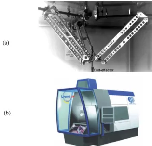
Let us demonstrate the efficiency of our design approach on a concrete problem coming from the industrial sector of the region of Nantes (France). One of the most important activity areas of this region is the manufacturing of bathroom components (shower cabin, washbasin, bathtub, etc. – Fig. 4). Most of parts used during the assembly process of the bathroom component are flat and made of thermosetting materials. The main operations achieved on these parts is trimming, i.e. the suppression of the edges of the parts in order to obtain a good surface roughness.
The machines tools that are used for the trimming of these bathroom components must be designed such as they attain the following characteristics:
- workspace Wabc of size {2.5 m × 2.5 m × 0.5 m};
- ||vxy|| = 60 m/min, ||fxy|| = 300 N and ||pxy|| = 0.25 mm
(fxy and pxy are the components of vectors f and p in
the xy plane).
Fig. 4. Typical examples of bathroom components manufactured in the region of Nantes (France).
experience, several types of robots may be envisaged, such as the Y-STAR [15], the UraneSX [16], the Orthoglide [3], the Hybridglide [17], the 3-UPU [18], etc. However, because the workspace is not a cube, but a flat parallelepiped, it appears that only two kinds of architectures, that have non-orthogonal arrangement of legs and that are already used in machining process, seem to be best adapted: the Y-STAR and the UraneSX (Fig. 5). It should be mentioned that, in our study, the prismatic guides of the UraneSX are vertical.
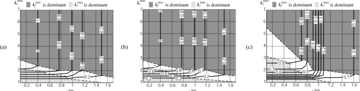
B. Comparison between the alternative solutions
Let us first compare the size of the workspace of the Y-STAR and the UraneSX in general cases, i.e. for many given maximal admissible values of the transmission factors. To apply the proposed design approach, let us normalize the problem by dividing the size of the workspace by 2.5 m such as the normalized workspace W0 is of dimension {1 × 1 ×
0.2} and by taking into account that the length of the legs of the mechanisms are identical and equal to 1.
Taking into account the general design objective, the scale factor µ may be optimized1. The results are plotted at
Figs. 6 and 7.
It follows from these results that the curves may be decomposed into three parts. In the first part (in bright gray), the variation of min
f
k has no (or very few) influence on the value of µ. Therefore, this zone corresponds to the area where max
v
k is the dominant parameter. In the second part (in dark gray), the variation of max
v
k has no (or very few) influence on the value of µ. Therefore, this zone corresponds to the area where min
f
k is the dominant parameter. The third zone is the area between the two others, i.e. where none of the two parameters are dominating. It may be seen that the borders of the two zones of dominance seems to have the form of hyperbolic portions of curves, which correlates the comments of section III.E on the duality between the parameters min
f
k and max
v
k .
The obtained results allow comparing the value of µ for the Y-STAR and the UraneSX. It appears that the scale factor µ of the Y-STAR is mostly superior than that of the
1 In the case of the UraneSX, the scale factor µ depends also on the radius R
of circumcircle of the base triangle. But, we consider that the value of the scale factor is defined as the maximum of µ for any given R.
(a)
(b)
Fig. 5. The robots under study: (a) Y-STAR and (b) UraneSX.
UraneSX, which implies that, for identical workspaces, the UraneSX will have legs of size greater than the Y-STAR, thus leading to larger deformations of the robot. But, before giving final conclusions on these two robots, other constraints coming from requirements that take into account the entire manufacturing cell should be considered.
C. Optimization results for bathroom components milling For the design of these two robots, actuated prismatic tables have to be used. The admissible velocity found in manufacturers’ catalogues for long prismatic tables is about vt =150 m/min, and their common minimal payload along
their axis is of ft = 3000 N for ball-screw systems. Moreover,
the accuracy of these pairs is about at = 0.05 mm. Therefore,
it was found that min
f
k = ||fxy|| / ft = 0.1, kvmin = ||vxy|| / vt =0.4
and max
v
k = ||pxy|| / at = 5.
Extracting µ from the previous general results and then scaling the robot taking into account that the corresponding normalized workspace is equal to µ W0, the lengths of legs
are obtained. They are of 2.16 m for the Y-STAR and of 4.62 m for the UraneSX. It is clear here that the Y-STAR will have smaller legs, and as a result, potentially a smaller loss of accuracy due to deformations, than the UraneSX. However, it could be shown that the footprint surface needed in order to install the Y-STAR is about two times bigger than for the UraneSX. Therefore, it looks more attractive to use the UraneSX in order to save some place on ground in manufacturing centres.
VI. CONCLUSIONS
In this paper, it has been proposed a new methodology for the optimal design of parallel kinematic machine tools. It is based on the concept of the maximal inscribed parallelepiped and uses technology-oriented constraints. To compute the parallelepiped, a dedicated combinatorial optimization algorithm is proposed. This approach is applied on two 3-DOF translational parallel robots: the Y-STAR and
the UraneSX. An analysis of the size of their workspace as a function of the design constraints is made. It is presented that, for workspaces with similar properties, the legs of the UraneSX are longer than for the Y-STAR, thus leading to greater deformations. However, it is shown that the footprint surface needed in order to install the Y-STAR is about two times bigger than for the UraneSX. Therefore, it may be interesting to use the UraneSX in order to save some place on ground in manufacturing centres.
ACKNOWLEDGMENTS
This work has been supported by the French région Pays de la Loire (RoboComposite project).
REFERENCES
[1] J.-P. Merlet, “Parallel robots,” Kluwer Academic Publishers, Dordrecht, 2000.
[2] J. Tlusty, J.C. Ziegert, and S. Ridgeway, “Fundamental comparison of the use of serial and parallel kinematics for machine tools,” CIRP
Annals, Vol. 48, No. 1, 1999, pp. 351–356.
[3] D. Chablat, P. Wenger, and J.-P. Merlet, “A Comparative Study between Two Three-DOF Parallel Kinematic Machines using Kinetostatic Criteria and Interval Analysis”, 11th World Congress in
Mechanism and Machine Science, Tianjin, China, 2004.
[4] L.W. Tsai, “Robot analysis: the mechanics of serial and parallel manipulators,” John Wiley and Sons, New York, 1999.
[5] I.A. Bonev, “The parallel mechanism information center,” available from: <http://www.parallemic.org>.
[6] J. Kim, and C. Park, “Performance analysis of parallel manipulator architectures for CNC machining applications,” Proceedings of the
IMECE Symposium on Machine Tools, Dallas, TX, 1997.
[7] Ph. Wenger, C.M. Gosselin, and D. Chablat, “A comparative study of parallel kinematic architectures for machining applications,”
Proceedings of the 2nd Workshop on Computational Kinematics,
Seoul, Korea, 2001, pp. 249–258.
[8] F. Rehsteiner, R. Neugebauer, S. Spiewak, and F. Wieland, “Putting parallel kinematics machines (PKM) to productive work,” CIRP
Annals 48, Vol. 1, 1999, pp. 345–350.
[9] C.-M. Luh, F.A. Adkins, E.J. Haug, and C.C. Qui, “Working capability analysis of Stewart platforms,” Journal of Mechanical
Design, Vol. 118, No. 6, 1996, pp. 89–91.
[10] J.-P. Merlet, “Determination of 6D workspace of Gough-type parallel manipulator and comparison between different geometries,”
International Journal of Robotics Research, Vol. 19, No. 9, 1999, pp.
902–916.
[11] X.-J. Liu, J. Wang, and G. Pritschow, “Performance atlases and optimum design of planar 5R symmetrical parallel mechanisms,”
Mechanism and Machine Theory, Vol. 41, No. 2, 2006, pp. 119–144.
[12] A. Pashkevich, D. Chablat, and P. Wenger, “Design optimization of parallel manipulators for high-speed precision machining applications,” Proceedings of the 13th IFAC Symposium on
Information Control Problems in Manufacturing (INCOM’2009),
Moscow, Russia, 2009, pp. 139–144.
[13] J.-P. Merlet, “Jacobian, manipulability, condition number, and accuracy of parallel robots,” Transaction of the ASME Journal of
Mechanical Design, 2006, Vol. 128, No. 1, pp. 199–206.
[14] J.-P. Merlet, “Computing the worst case accuracy of a PKM over a workspace or a trajectory,” The 5th Chemnitz Parallel Kinematics
Seminar, Chemnitz, Germany, 2006, pp. 83–96.
[15] J.M. Hervé, “Group mathematics and parallel link mechanisms,”
IMACS/SICE International Symposium on Robotics, Mechatronics, and Manufacturing Systems, Kobe, Japan, 1992, pp. 459–464.
[16] O. Company, and F. Pierrot, “Modelling and design issues of a 3-axis parallel machine-tool,” Mechanism and Machine Theory, Vol. 37, 2002, pp. 1325–1345.
[17] O. Company, “Machine-Outils Rapides à Structure Parallèle. Méthodologie de Conception, Applications et Nouveaux Concepts,” PhD thesis, Montpellier University, 2000.
[18] L.W. Tsai, and S. Joshi, “Kinematics and Optimization of a Spatial 3-UPU Parallel Manipulator,” Journal of Mechanical Design, Vol. 122, No. 1, 2000, p. 5–11.
(a) (b) (c)
Fig. 6. Values of the scale coefficient µ for the Y-STAR robot as a function of min
f
k and max
v
k , for (a) min
v k = 0.2, (b) min v k = 0.4 and (c) min v k = 0.6. (a) (b) (c)
Fig. 7. Values of the scale coefficient µ for the UraneSX robot as a function of min
f
k and max
v
k , for (a) min
v k = 0.2, (b) min v k = 0.4 and (c) min v k = 0.6.