An innovative technique for real-time adjusting exposure time of silicon-based camera to get stable gray level images with temperature evolution

HAL Id: hal-02131320

https://hal.archives-ouvertes.fr/hal-02131320

Submitted on 16 May 2019

HAL is a multi-disciplinary open access

archive for the deposit and dissemination of sci-entific research documents, whether they are pub-lished or not. The documents may come from teaching and research institutions in France or abroad, or from public or private research centers.

L’archive ouverte pluridisciplinaire HAL, est destinée au dépôt et à la diffusion de documents scientifiques de niveau recherche, publiés ou non, émanant des établissements d’enseignement et de recherche français ou étrangers, des laboratoires publics ou privés.

An innovative technique for real-time adjusting exposure

time of silicon-based camera to get stable gray level

images with temperature evolution

Chao Zhang, Jérémy Marty, Anne Maynadier, Philippe Chaudet, Julien

Réthoré, Marie-Christine Baietto

To cite this version:

Chao Zhang, Jérémy Marty, Anne Maynadier, Philippe Chaudet, Julien Réthoré, et al.. An innovative technique for real-time adjusting exposure time of silicon-based camera to get stable gray level images with temperature evolution. Mechanical Systems and Signal Processing, Elsevier, 2019, 122, pp.419 -432. �10.1016/j.ymssp.2018.12.042�. �hal-02131320�

1

An innovative technique for real-time adjusting exposure time of

silicon-based camera to get stable gray level images with temperature evolution

C. Zhang a,*, J. Marty a,b, A. Maynadier c, P. Chaudet a, J. Réthoré d, M.C. Baietto a a. Department of Mechanical Engineering, LaMCos, Université de Lyon/INSA Lyon/UMR

CNRS 5259, 20 Avenue des Sciences, F-69621 Villeurbanne Cedex, France. b. ESTA LAB, 3 Rue du Dr Frery, F-90000 Belfort, France

c. Univ. Bourgogne Franche-Comté, FEMTO-ST Institute, CNRS/UFC/ENSMM/UTBM, Department of Applied Mechanics, Chemin de L'épitaphe, 25000 Besançon, France d. GeM, Centrale Nantes/Université de Nantes/UMR CNRS 6183, 1 rue de la Noë, BP 92101,

F-44321 Nantes, France

* Corresponding email: chao.zhang@insa-lyon.fr

Abstract

Silicon-based sensor cameras are known to be sensitive in the near infrared spectral range, in which a small temperature variation leads to a large modification in the image gray level. It induces acquired images with local saturation or poor dynamic range of gray levels. In order to address this problem, the present study proposes an innovative technique to precisely and automatically adjust the exposure time to obtain stable gray level images when the temperature evolution occurs on the surface of the observed object. Two algorithms, including linear algorithm and Planck’s algorithm, are proposed to predict the exposure time to obtain stable gray level images. Blackbody heating experiment is conducted to validate the accuracy of these two algorithms, and the result indicates that stable gray level images can be obtained using Planck’s algorithm. Moreover, this technique is applied to the specimen heating experiment, and the stable gray level images can also be obtained using Planck’s algorithm. These two experimental results prove that the technique is effective and reliable. Finally, the thermal fields are reconstructed on images of blackbody.

2

Keywords: Silicon-based camera; Exposure time adjustment; Planck’s algorithm; Thermal

field

1. Introduction

Nowadays, experimental science is faced with major multiphysical challenges (particularly thermo-mechanical) requiring the development of advanced test benches, multiplying the use of in-situ measurement techniques. Simultaneous measurement of thermal and kinematic full fields are considerably developing. Measuring precisely temperature distribution on the surface of an object undergoing thermal cycle is very important in many fields, such as thermo-mechanics [1, 2] and thermophysics [3, 4], etc. Many techniques have been developed to measure temperature, e.g., thermocouple [5, 6], thermistor [7], resistance temperature detector [8], and infrared thermography [9-12], etc. Among these methods, infrared thermography is an advanced non-contact full-field measurement technique. It transforms the thermal radiation, emitted by objects in the infrared wavelength of the electromagnetic spectrum (i.e. from 1 to 1000 μm), into an electronic video signal with a resolution depending on the physical size of each pixel and of the whole sensor [13-17]. Nevertheless, the common infrared cameras operate in the middle wave infrared spectral range (MWIR) in order to have the best sensitivity for temperature in the ambient vicinity. It nonetheless presents some essential problems. First of all, because of its preliminary calibration on a blackbody (emissivity ε ≈ 1), the technique assumes that the infrared flux received from the surface of the observed object is only due to its thermal state, i.e. that the surface is assumed to have a perfect emissivity. It induces two practical issues:

- the object should present uniform, flat and constant emissivity. Some materials, without artifice, present satisfying emissivity (polished glass ε ≈ 0.8 to 0.9, some polymers or rubber ε ≈ 0.85 to 0.95). For specimen where emissivity is too low or

3

heterogeneous, coating with dedicated paint or black carbon powder is required, eventually masking local thin scale surface phenomena.

- if the emissivity is not maximal, radiation from surrounding objects (depending on their own temperature) can reflect on the target object and be misinterpreted. Thus disturbance due to the surrounding radiation should be measured but the required correction is difficult to define because of the lack of knowledge of the different temperatures and emissivity involved.

To avoid these two main disadvantages of mid-wave infrared thermography, it is effective to operate in lower spectral range (near infrared spectral range). Teyssieux et al. [18, 19] proposed that the disturbance due to radiation from surrounding objects is low and can be negligible when the wavelength is less than 2 μm, while the disturbance radiation from surrounding objects is obvious when the wavelength is greater than 2 μm. Their study indicated that disturbance due to radiation from surrounding objects can be ignored using lower spectral range. Rotrou et al. [20] studied the measurement of thermal fields of an object with non-homogeneous emissivity by both infrared camera (operating in the spectral ranges of 8-12 μm) and silicon-based camera (operating in the spectral ranges of 0.7-1.1 μm). The results show that the more accurate thermal field can be obtained using silicon-based camera with processing in a lower spectral range, while larger errors appear using infrared camera. To sum up, cameras equipped with silicon detectors are usually operating in the visible spectrum (0.4-0.7 μm), and widely used to perform real-time observation of the kinematic fields, mainly thanks to digital image correlation or interferometry [21-27]. The silicon-based cameras are also operating in near infrared spectrum (0.7-1.1 μm) [28, 29]. Thus, they are good candidates to measure both kinematical and thermal fields for high temperature applications if the sensors are properly calibrated. Compared with a dedicated infrared camera, a silicon-based camera is cheaper, presents lower noise, possesses a longer durability

4

and has major advantage to deliver a far higher resolution (about 4800×3600 pixels). Thus, it has been used for industrial applications [30, 31].

Nonetheless, it subsists one main disadvantage for silicon-based cameras: in the near infrared spectral range the gray level of the acquired image changes fast even with small temperature variation. Orteu et al [32] gave an example: for wavelength around 1 μm, the ratio of the measured gray level between 573K and 1273K is about one million (times), whereas in the long-wave infrared spectral range (10 μm) the ratio is only five (times). This high sensitivity to temperature variation leads to poor quality images due to oversaturation and/or poor dynamic range of gray levels. This phenomenon will destroy the images, and any useful information cannot be obtained.

In this study, we propose a technique to precisely and automatically adjust the exposure time of a silicon-based camera to obtain stable gray level images whatever the temperature evolution occurs. The technique is validated by both blackbody heating experiment and specimen heating experiment.

2. Experiments

2.1 Experimental set-up

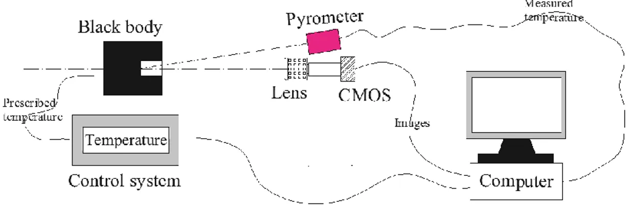
The schematic diagram of the blackbody experimental set-up is shown in Fig. 1. This is composed of four main elements: (a) a blackbody (temperature reference source up to 1350

K) and its temperature controller (RCN 1200 N1 manufactured by HGH); (b) a 8bits CMOS camera (Viewworks VC-12MC) with 4096 × 3072 pixels, mounted with a lens (Nikon ED, 200 mm); (c) a computer which controls the image acquisition and records the experimental data (image, blackbody internal temperature, exposure time); and (d) the blackbody internal temperature is measured by a pyrometer, while the theoretical temperature of the blackbody is prescribed by the temperature controller.

5

The experiments are performed in a dark room without the interference of other heat sources. The CMOS camera is placed with its optical axis normal to the 50 mm aperture of the blackbody. The distance between the front lens of the camera and the blackbody is about 1 meter. The CMOS camera is controlled by home-made Labview software. The software not only controls the image acquisition time but also automatically adjusts the exposure time of the camera to obtain stable gray level images during the heating process of blackbody. The computer records simultaneously the digital images acquired by the camera (with gray level encoded between 0 and 255 level), exposure time of the camera and the acquisition time.

Fig. 1 Blackbody experimental set-up. 2.2 Radiometric model

Silicon-based camera receives the incident flux coming from the target object which is

related to its surface temperature. Each pixel then converts the incident flux into the output signal (gray level value), so the gray level value of image is directly affected by the temperature. Meanwhile, the exposure time is also related to the duration of acquisition and thus to the amount of photons collected by the sensor, thus the obtained gray level of an image can be modified by adjusting the exposure time of camera. Establishing the relationship among exposure time, temperature and gray level is the first step to use a silicon-based camera to perform near infrared thermography. Fig. 2 shows an acquired image, in which the red square area is the region of interest (ROI) with 1000 × 1000 pixels. A set of images have been recorded (with manual adjustment of exposure time and temperature) when blackbody

6

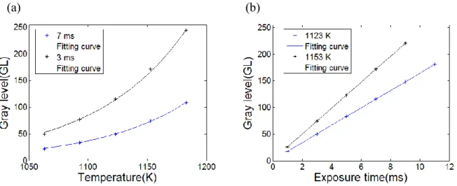
temperature and exposure time are independently varied between [1050; 1250K] (for fixed exposure times of 7 ms and 3 ms) and [1; 11 ms] (for fixed temperatures of 1123K and 1153K) respectively. Fig. 3(a) shows the evolution of mean gray level of ROI as a function of temperature. One can observe that mean gray level increases faster with the increasing of the temperature. The evolution of mean gray level as a function of the exposure time for fixed temperatures of 1123K and 1153K is also shown in Fig. 3(b). A linear relationship between gray level and exposure time can be observed.

Fig. 2 Image acquired by camera and the ROI with 1000 × 1000 pixels.

Fig. 3 (a) Evolution of mean gray level of ROI as a function of temperature for exposure times of 7 ms and 3 ms;

and (b) evolution of mean gray level of ROI as a function of exposure time for temperatures of 1223K and

1253K.

Radiometric model describes the relationship among exposure time, temperature and gray level. In this case, the radiometric model (the detailed derivation is presented in Appendix 1) can be written as follows [32]:

7 _{( )} ( ) _exp( 2 ₎ ( ) n w x C I T I T k T T      ₍₁₎

where I Tn( ) is the intensity, ( )I T is the gray level,



is the exposure time of camera, C2 is

the second Planck’s constant (1.44 × 10-2 _{m·K), T is the absolute temperature. k}

w is a

parameter of the camera which should be determined by radiometric calibration process.

 

x T

 is the extended effective wavelength introduced into the radiometric model because the spectral density of energy in the near infrared spectral band will move to lower

wavelengths when the temperature increases. It is worth noting that the intensity I T_n( ),

which is defined as gray level I T( ) divided by exposure time  , is introduced in the radiometric model to avoid performing too many radiometric model calibrations for all different exposure times. Meanwhile, theextended effective wavelength x

 

T is defined by the following equation [33]:

 

0 1 22





1 , 0 n n x a a a a n T T T T         (2) where a0, a1, a2, ···, an are parameters, which should be determined by calibration process.

In this case a narrow temperature range of 200 K is studied, so the extended effective wavelength with two parameters a0 and a1 is enough [32]. Thus, the radiometric model can be

written as follows: 2 0 2 1 2

( )

( )

exp(

)

n w

C

a

C

a

I T

I T

k

T

T















(3) Blackbody experiments (13 images acquired with manual adjustment of blackbody temperature and exposure time) are conducted to calibrate the radiometric model. In this study, the least square method is used to calibrate the radiometric model of blackbody. Through the calibration process, three parameters of radiometric model of blackbody are

8

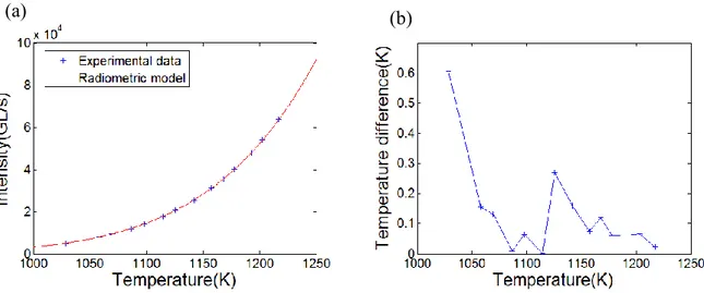
obtained and indicated in Table 1. The calibrated radiometric model of blackbody is shown in Fig. 4(a), in which the experimental data follows well the calibrated radiometric model.

Table 1 The three parameters of radiometric model of blackbody. kw (GL/s) a0 (m-1) a1 (K·m-1)

1.358×1011 _1.28×106 _-5.9368×107

In order to validate the radiometric calibration, the temperature difference of the

radiometric model Tradio is calculated, which is defined by:

Tradio  TrealTradio (4)

where Treal is the temperature measured by the pyrometer; Tradio is the calculated temperature

based on radiometric model. Fig. 4(b) shows the temperature differences at different

measured temperatures. The maximum difference is only 0.6 K, which is less than 0.06% of the measured temperature.

Fig. 4 (a) Radiometric model and experimental data; and (b) temperature differences of the radiometric model at different measured temperatures.

3. Approach to control image gray level

3.1 Basic principle of the approach

9

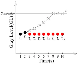
The objective of the new approach is to continuously and automatically adjust the exposure time to get a set of stable gray level images whatever the temperature evolution is. The principle of the proposed approach is schematically shown in Fig. 5. At the beginning, the first two images (as indicated by black points) are acquired with an identical exposure time (i.e., τ1 = τ2 = τ). If exposure time is kept unchanged while the temperature increases, the

image gray level will increase fast (as indicated by the hollow points) to saturation. Thus, the exposure time should be adjusted (decreased in this situation) to make the image gray level equal to that of the first image (as indicated by red points).

Fig. 5 Schematic diagram of the basic principle of the approach. 3.2 Detailed procedure of the exposure time adjustment

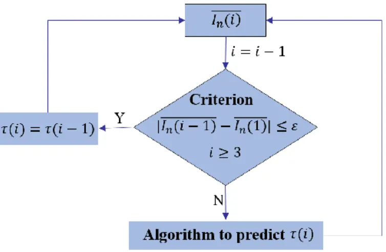
It is observed from the radiometric model that the intensity is only related to temperature. If the first two images are known, the intensity of the third one can be predicted. The flow chart for controlling the image gray level is shown in Fig. 6. A criterion equation is introduced as follows:

I i_n(  1) I_n(1) ,i3 (5)

where I i _n( 1) is the mean intensity of image number i 1, I_n(1) is the mean intensity of the

10

cannot be exactly zero as it is impossible to acquire two exactly identical images in reality (noise, vibrations, optical disturbance, etc.).

When the discrepancy in mean intensity between the image i 1 and the first one is less than the critical value ε, it means that the temperatures between these two images are almost

the same. Thus, it is unnecessary to adjust the exposure time and the next exposure time  ( )i

can be equal to the last one (i1). When the discrepancy is greater than the critical value ε, it means that the temperatures between these two images are different. The exposure time should be adjusted to make the gray level equal to that of the first one. In this situation, an algorithm to accurately predict the next exposure time should be given. This study proposes two algorithms (Linear algorithm and Planck’s algorithm) in the following section to predict

the next exposure time  . ( )i

Fig. 6 Flow chart of the approach to control the image gray level. 3.3 Two possible algorithms to predict the next exposure time

Linear algorithm: A linear algorithm can be used to predict the next exposure time.

When the frequency of camera is maintained constant, the next mean intensity I i_n( )can be

given based on the specific law of linear function:

( ) 2 ( 1) ( 2)

n n n

I i  I i I i (6)

11 ( ) ( 1) ( 2) ( ) 2 ( ) ( 1) ( 2) n I i I i I i I i i i i            (7)

In order to make sure that mean gray level of image number i is equal to that of the first image

( ) (1)

I i I , the next exposure time can be predicted by:

(1) ( ) ( 1) ( 2) 2 ( 1) ( 2) I i I i I i i i           (8)

Planck’s algorithm: The radiometric model is derived from the Planck’s law, and its basic equation is an exponential function. Thus, the exponential algorithm based on Planck’s

law is used to predict the next exposure time. When the frequency of camera is maintained

constant, the next intensity of image can be given based on the specific law of exponential function: 2 ( 1) ( ) ( 2) n n n I i I i I i    (9)

Eq. (9) can be expanded:

2 ( ) ( 1) ( 2) ( ) ( ) ( 1) ( 2) n I i I i i I i i i I i         _{ }      (10)

In order to make sure that mean gray level of image number i is equal to that of the first image

( ) (1)

I i I , the next exposure time can be predicted by:

2 ( 1) ( 2) ( ) (1) ( 2) ( 1) i I i i I i I i         _{ }      (11)

Based on Eqs. (8) and (11), a software is made to automatically adjust exposure time.

4. Validation and comparison of two algorithms

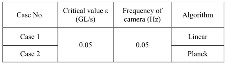
Blackbody heating experiments are conducted with a temperature range from 1024K to 1224K. Eighteen images are acquired with automatic adjustment of exposure time by the homemade software. The objective is to validate and compare the accuracy of two algorithms

12

proposed above. The parameters of the two cases are shown in Table 2. A set of simulated grey levels, inferred from the radiometric model, are firstly obtained by Matlab software.

Then a set of realistic images during blackbody heating experiments at the same conditions as

the simulation are obtained to be compared with the simulated ones. We aim at quantify how

much both algorithms are able to keep the stable mean gray level of ROI whatever the temperature evolution is.

Table 2 The parameters of two cases to validate and compare two algorithms. Case No. Critical value ε _(GL/s) Frequency of _{camera (Hz)} Algorithm

Case 1

0.05 0.05 Linear

Case 2 Planck

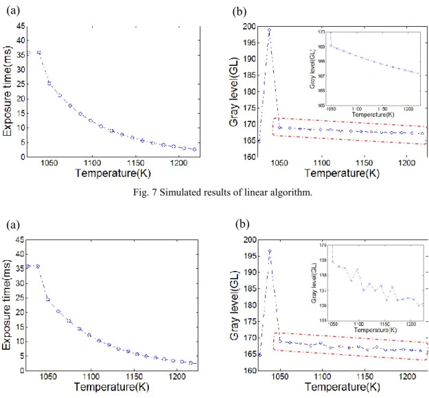
Case 1: Based on the radiometric model of blackbody and the linear algorithm to

predict the next exposure time, the simulation process is conducted by Matlab software. Fig. 7 shows the simulated results of case 1 by using linear algorithm. The first two images are taken with a constant exposure time (about 35.1 ms). It is observed from Fig. 7(b) that the image gray level rapidly increases with the increasing of temperature. When the linear algorithm operates and automatically adjusts the exposure time after the second image, it can be seen

from Fig. 7(a) that the exposure time rapidly decreases when the temperature increases, and

the corresponding gray level in Fig. 7(b) decreases. Meanwhile, the evolution of gray level after adjustment (as indicated by dotted line rectangle) is magnified. From the magnified image, it is worth noting that the first exposure time adjustment is underestimated leading to a mean gray level a little bit higher than expected (error of 2%). Nonetheless the gray level then decreases to converge till the first image average gray level.

Blackbody heating experiments with the same conditions as the simulation process are conducted, and the experimental results are shown in Fig. 8. Comparing the experimental

13

results (Fig. 8) with the simulated ones (Fig. 7), one can observe that the evolution of exposure time (Fig. 8(a)) and gray level (Fig. 8(b)) in the experiments is almost the same with that of simulated results, but the difference is that the gray level after adjustment in the magnified image is not a perfectly linear reduction relationship due to the noises.

Fig. 7 Simulated results of linear algorithm.

Fig. 8 Experimental results of linear algorithm.

Case 2: The Planck’s algorithm is also used to maintain the gray level stable as the

temperature increases. Fig. 9 shows simulated results of exposure time and mean gray level of ROI by using Planck’s algorithm. The exposure time is constant for the two first images (33.5 ms), so the 2nd _{mean grey level is quite different from that of first one. The gray level then}

decreases to be almost equal to that of the first image due to the rapid decrease of the

(a) (b)

14

exposure time (Fig. 9(a)). The magnified image in Fig. 9(b) indicates that a stable gray level

after adjustment is obtained.

Based on Planck’s algorithm, the corresponding experimental results at the same conditions are shown in Fig. 10. It is apparent that the evolution of exposure time (Fig. 10(a)) and gray level (Fig. 10(b)) with the increasing of temperature agrees well with the simulated one, and the image gray level after adjustment decreases to the original value of the first image.

Fig. 9 Simulated results of Planck’s algorithm.

Fig. 10 Experimental results of Planck’s algorithm.

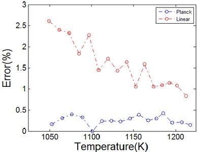
The error, which is defined as the difference between mean gray level of image and the mean gray level of first image normalized by the mean gray level of first image, is introduced as follows:

(a) (b)

15 ( ) (1) 100% (1) I i I error I    (12)

Both experimental errors of linear algorithm and Planck’s algorithm are depicted in Fig. 11. It is apparent that the Planck’s algorithm has two advantages: (1) the errors are less than 0.5% which is much smaller than the linear algorithm; (2) the errors are stable. This result indicates that the Planck’s algorithm based on the radiometric model is better to predict precisely the next exposure time, thereby resulting in the more accurate image gray levels equal to that of the first image after exposure time adjustment.

Fig. 11 Experimental errors of linear algorithm and Planck’s algorithm.

5. Realistic application of this technique

5.1 Specimen heating experiment

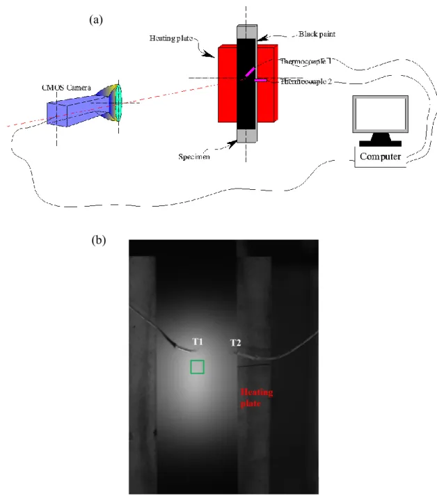
The material used is Ti-6Al-4V titanium alloy, of which the chemical composition (wt.-%) is Ti-6.05Al-4.32V-0.22Fe-0.04Si-0.024C-0.006N-0.16O-0.003H. A specimen with dimensions of 100 mm (length) × 10 mm (width) × 1 mm (thickness) was cut from the sheets. The specimen surface was sprayed by the black paint.

Fig. 12(a) shows the experimental set-up. The distance between the front lens of the camera and the specimen surface was 1 meter. A thermocouple (T2) was welded at the edge

16

of the specimen, while another one (T1) was welded in the center of the specimen. The temperature of heating plate was controlled from 873 K to 1023 K and the heating rate is set to 5 K/s. The distance between heating plate and specimen is 0.1 meter. The software based on the Planck’s algorithm is used for automatic adjustment of exposure time and the images are acquired at the same time. Fig. 12(b) shows an acquired image of specimen surface. Green rectangle is a chosen ROI with 200 × 200 pixels, of which the mean gray level is intended to be maintained stable or even constant by automatic adjustment of exposure time.

Fig. 12 (a) Experimental set-up; and (b) acquired image of specimen surface.

(a)

17 5.2 Control of image gray level

Fig. 13(a) shows the evolution of mean gray level of ROI with/without exposure time adjustment. The red points indicates that without exposure time adjustment the mean gray level of ROI increases fast from original gray level 180 GL to the maximum gray level 255 GL as the temperature of T2 increases from 837 K to 846 K. As the temperature further increases, the saturated images will be obtained without any useful information. As indicated by blue points, with exposure time adjustment the mean gray level of ROI maintain almost constant as the temperature of T2 increases from 837 K to 962 K. The corresponding exposure time after automatic adjustment of exposure time during heating process is shown in Fig. 13(b), in which the exposure time decreases to maintain the gray level stable when the temperature increases. These results further indicate that the algorithm and software are feasible and reliable.

Fig. 13 (a) Mean gray level of ROI and (b) exposure time evolves as the temperature of T2 increases with/without exposure time adjustment.

6. Thermal fields

Thermal fields on the ROI of blackbody images are reconstructed. Fig. 14 shows the

comparisons between the mean temperatures Tcal calculated from the mean gray level of ROI

by radiometric model of blackbody and the measured pyrometer temperatures Treal when

18

using the Planck’s algorithm for exposure time adjustment. Fig. 14(a) permits to conclude that the calculated mean temperatures are in good agreement with the measured temperatures. To

be more precise, the temperature difference Tmean defined as Tmean  TrealTcal is plotted in

Fig. 14(b) at different measured temperatures. One can observe that most of temperature differences are less than 1 K (about 0.1% of the measured temperature), which validates the high accuracy of this near infrared thermography technique.

Each pixel is an elementary photon flux sensor, so the thermal field can also be computed pixelwise based on radiometric model of blackbody. Some examples of thermal fields at various measured temperatures are shown in Fig 15. Meanwhile, the temperature difference

pixel

T

 between pixel temperature and measured temperature is defined as

pixel real pixel

T T T

   . The error fields at various pyrometer temperatures are also depicted in

Fig. 15. It is apparent that the error fields at various measured temperatures are uniform and relatively low, and most of error values are less than 1 K (0.1% of the measure temperature). It also demonstrates the high accuracy of this near infrared thermography technique.

Fig. 14 (a) Comparison between calculated and measured temperatures; (b) temperature differences at various measured temperatures.

19

Temperature

(K) Thermal fields (K) Error fields (K)

1064.7

1111.8

1166.9

1187.8

1228.0

Fig. 15 Reconstructed thermal fields and error fields from recorded images with in situ mean gray level conservation (Planck’s algorithm).

20

7. Conclusions

In this study, the radiometric model of blackbody is calibrated by least square method, and the radiometric model of blackbody with three parameters kw, a0 and a1 is obtained. Meanwhile, the errors of radiometric model at different temperatures are also calculated, and the maximum error is only 0.6 K which is about 0.06% of the measured temperature. An innovative technique to precisely and automatically adjust the exposure time of CMOS camera to obtain a kinematically and thermally exploitable image whatever the temperature

evolution on the surface of the observed object is. Two algorithms, including linear algorithm

and Planck’s algorithm, are proposed to predict the exposure time of next image. A software based on both linear algorithm and Planck’s algorithm is made and used in the blackbody heating experiments. The experimental result indicates that the stable image gray level can be obtained by using Planck’s algorithm based on the radiometric model; while larger errors will occur by using linear algorithm. This new technique is also applied to a realistic specimen heating experiment. The result shows that the images with stable gray levels can be acquired with the software based on the Planck’s algorithm. Finally, the thermal fields of blackbody images acquired at various temperatures can be reconstructed based on the radiometric model of blackbody. Both mean temperature differences and pixel temperature differences at various temperatures are almost less than 1K.

Appendix 1

Principle of radiometric model

The surface of any object has its own emissivity (0 <  

 

< 1) and own temperature (T > 0 K). It emits electromagnetic energy in the form of radiation in a wavelength range [λ1, λ2].

The Planck’s law describes the total monochromatic flux M



,T



emitted by a blackbody as

21

Planck’s law, the total monochromatic flux emitted by the surface of any object e with

uniform emissivity can be given as follows:





  



 

1 1 2 5 , , exp 1 e C C T M T T                   _{  } _     (A1)

where C1 is the first radiation constant (C1 = 3.7415×10-16 W·m2); c2 is the second radiation constant (C2 = 1.44×10-2 m·K).

In reality, the measurement of a flux emitted by a target surface is difficult to be achieved because the reflection of a flux from surrounding objects received by this surface

ref

 is often superimposed on it. The total flux received by a detector tot is therefore given

as follow:

_tot



,T



 _e



,T



 _ref



,T

   

  M ,T



 (1  

 

)_ref



,T



(A2) The quantum sensors of the detectors use the photoelectric effect to create electrons from the received photons if their energy is sufficient (greater than the gap energy of the material constituting the detector). The electron flow is measured during the exposure time for each of the pixels, which is finally converted to the form of digital level I. The detectors made by different materials can receive different wavelength range. For example, the silicon based detector can received the wavelength range from 0.4 μm to 1.1 μm, while the VisGaAs based detector can receive the wavelength range from 0.4 μm to 1.7 μm. In this case, the silicon-based camera is used due to its low cost, lack of cooling, low sensitivity to the emissivity of the material and its spatial resolution.

The description of the measurement chain makes it possible to establish the general radiometric equations. Cabannes [34] indicated that it is generally necessary to simplify these equations to be able to use them, and the equation can be reduced to the following two terms:

22

where



is the exposure time (integration time) of camera; W

 

 is the spectral response of the whole measurement system. Different systems has different components. Generally, the spectral response of the whole measurement system involves the spectral transmittance of the atmosphere atm, the spectral transmittance of the filter filter(if there is), the spectral quantum

efficiency e, and so on.

If the measurement is carried out in darkness room without other energy sources, the term ref can be considered as zero and ignored. Thus, the Eq. (2.3) can be given as follows:

    



   

1 1 2 5 , C exp C 1 I W M T d W d T                            _{  } _     





(A4)

In this study, the CMOS camera with maximum received wavelength of 1.1 μm is used, and the maximum temperature measured for the tests is 1203 K. Wien’s approximation indicates

that: if  T 2900m K , it can be simplified as exp C2 1 exp C2

T T

 

 _{ }  

   

   . Thus, this study

satisfies the condition of Wien’s approximation (1.1m1203K2900m K ), and the Eq. (A4) can be simplified as follows:

   

1 2 5 exp C C I W d T               _ _  



(A5)

To simplify the Eq. (A5), Rotrou [35] introduced an effective wavelength e into the

radiometric model. Thus, the digital signal I can be given as follows:

   



5



2 1 int e e e exp e C I c K W T                 _ _   (A6)

where the Kint is a integration constant. Based on the Saunders’s research [33], the extended

effective wavelength _x( )T is also introduced by Rotrou [35] into the term exp 2 e C T         to

23 2 exp ( ) w x C I k T T        _ _   (A7)

where the kw is a parameter which should be determined by radiometric calibration process, T

is the absolute temperature, C2 is the second Planck’s constant (1.44 × 10-2 m·K), x( )T is the

extended effective wavelength introduced into the radiometric model because the spectral density of energy in the near infrared spectral band will move to lower wavelengths when the temperature increases. The extended effective wavelength λx(T) is defined by the following equation [33]:

 

0 1 22





1 , 0 n n x a a a a n T T T T         (A8)

where a0, a1, a2, a3, ···, an are parameters dependent of the whole bench configuration camera’s sensor, lens, surrounding objects, etc.), which should be determined by a priori in situ radiometric calibration. Due to the short temperature range (less than 300 K) to be studied in this case, the extended effective wavelength with two parameters a0 and a1 is enough. Thus, the radiometric model equation can be written as follows:

2 0 2 1 2 exp w C a C a I k T T         _  _   (A9)

To avoid performing too many radiometric model calibrations for each exposure time, the intensity In, which is defined as gray level I divided by exposure time  , is introduced. Thus, the radiometric model equation can be written as follows:

2 0 2 1 2 exp n w C a C a I I k T T         _  _   (A10)

The Eq. (A10) is the radiometric model, which provides the desired relation between the temperature of the studied surface T and the gray level I, which should be calibrated and three parameters should be known in order to measure the temperature distribution of object surface.

24

References

[1] D. Palumbo, R. De Finis, G.P. Demelio, U. Galietti, Study of damage evolution in composite materials based on the thermoelastic phase analysis (TPA) method. Composites Part B: Engineering 117 (2017) 49-60.

[2] S. Sfarra, S. Perilli, D. Ambrosini, D. Paoletti, L. Nardi, T. De Rubeis, C. Santulli, A proposal of a new material for greenhouses on the basis of numerical, optical, thermal and mechanical approaches. Construction and Building Materials 155 (2017) 332-347.

[3] D. Riquet, N. Houel, J.L. Bodnar, Stimulated infrared thermography applied to differentiate scar tissue from peri-scar tissue: a preliminary study. Journal of Medical Engineering & Technology 40 (2016) 307-314.

[4] S. Perilli, S. Sfarra, D. Ambrosini, D. Paoletti, S. Mai, M. Scozzafava, Y. Yao, Combined experimental and computational approach for defect detection in precious walls built in indoor environments. International Journal of Thermal Sciences 129 (2018) 29-46.

[5] M. Genix, P.Vairac, B. Cretin. Local temperature surface measurement with intrinsic thermocouple. International Journal of Thermal Sciences 48 (2009) 1679-1682.

[6] D.D. Bloomquist, S.A. Sheffield, Thermocouple temperature measurements in shock compressed solids, Journal of Applied Physics 51 (1980) 5260-5266.

[7] J. Kim, J.D. Kim, Voltage divider resistance for high-resolution of the thermistor temperature measurement, Measurement 44 (2011) 2054-2059.

[8] N.J. Blasdel, Fabric nanocomposite resistance temperature detector, IEEE Sensors Journal 15 (2015) 300-306.

[9] X. Wang, J.F. Witz, A.E. Bartali, C. Jiang. Infrared thermography coupled with digital image correlation in studying plastic deformation on the mesoscale level. Optics and Lasers in Engineering 86 (2016) 264-274.

25

[10] T. Liu, W. Zhang, S. Yan. A novel image enhancement algorithm based on stationary wavelet transform for infrared thermography to the de-bonding defect in solid rocket motors. Mechanical Systems and Signal Processing 62-63 (2015) 366-380.

[11] X. Guo, Y. Mao. Defect identification based on parameter estimation of histogram in ultrasonic IR thermography. Mechanical Systems and Signal Processing 58-59 (2015) 218-227.

[12] Y.W. Qin, N.K. Bao. Infrared thermography and its application in the NDT of sandwich structures. Optics and Lasers in Engineering 25 (1996) 205-211.

[13] T. Astarita, G. Cardone, G.M. Carlomagno. Infrared thermography: An optical method in heat transfer and fluid flow visualization. Optics and Lasers in Engineering 44 (2006) 261-281.

[14] C. Bougriou, R. Bessaih, R. Le Gall, J.C. Solecki. Measurement of the temperature distribution on a circular plane fin by infrared thermography technique. Applied Thermal Engineering 24 (2004) 813-825.

[15] Z. Ge, X. Du, L. Yang, Y. Yang, Y. Li, Y. Jin. Performance monitoring of direct air-cooled power generating unit with infrared thermography. Applied Thermal Engineering 31 (2011) 418-424.

[16] M.B. Janetti, L.P.M. Colombo, F. Ochs, W. Feist. Determination of the water retention curve from drying experiments using infrared thermography: A preliminary study. International Journal of Thermal Sciences 114 (2017) 271-280.

[17] J.H. Tan, E.Y.K. Ng, U. Rajendra Acharya, C. Chee. Infrared thermography on ocular surface temperature: A review. Infrared Physics & Technology 52 (2009) 97-108.

[18] D. Teyssieux, D. Briand, J. Charnay, N.F. de Rooij, B. Cretin, Dynamic and static thermal study of micromachined heaters: the advantages of visible and near-infrared

26

thermography compared to classical methods, Journal of Micromechanics and Microengineering 18 (2008) 065005.

[19] D. Teyssieux, S. Euphrasie, B. Cretin. Thermal detectivity enhancement of visible and near infrared thermography by using super-resolution algorithm: Possibility to generalize the method to other domains. Journal of Applied Physics 105 (2009) 064911.

[20] Y. Rotrou, T. Sentenac, Y. Le Maoult, P. Magnan, J. Farre, Demonstration of near infrared thermography with silicon image sensor cameras. Proceedings of SPIE - The International Society for Optical Engineering 5782 (2005) 9-18

[21] M. Bornert, P. Doumalin, J.C. Dupre, C. Poilane, et al. Shortcut in DIC error assessment induced by image interpolation used for subpixel shifting. Optics and Lasers in Engineering 91 (2017) 124-133.

[22] R. Hinady, M. Hagara. A new procedure of modal parameter estimation for high-speed digital image correlation. Mechanical Systems and Signal Processing 93 (2017) 66-79. [23] J. Zhang, A. Sweedy, F. Gitzhofer, G. Baroud. A novel method for repeatedly generating

speckle patterns used in digital image correlation. Optics and Lasers in Engineering 100 (2018) 259-166.

[24] X. Guo, Y. Li, T. Suo, H. Liu, C. Zhang. Dynamic deformation image de-blurring and image processing for digital imaging correlation measurement. Optics and Lasers in Engineering 98 (2017) 23-30.

[25] L. Felipe-Sese, F.A. Diaz. Damage methodology approach on a composite panel based on a combination of Fringe projection and 2D digital image correlation. Mechanical Systems and Signal Processing 101 (2018) 467-479.

[26] L. Yu, B. Pan. Single-camera high-speed stereo-digital image correlation for full field vibration measurement. Mechanical Systems and Signal Processing 94 (2017) 374-383.

27

[27] C.P. Goh, H. Ismail, K.S. Yen, M.M. Ratnam. Single-step scanner-based digital image correlation (SB-DIC) method for large deformation mapping in rubber. Optics and Lasers in Engineering 88 (2017) 167-177.

[28] K. Mangold, J. A Shaw, M. Vollmer. The physics of near-infrared photography. European Journal of Physics 34 (2013) S51-S71.

[29] F. Meriaudeau. Real time multispectral high temperature measurement: Application to control in the industry. Image and Vision Computing 25 (2007) 1124-1133.

[30] S. Price, K. Cooper, K. Chou, Evaluations of temperature measurements in powder-based electron beam additive manufacturing by near-infrared thermography. International Journal of Rapid Manufacturing 4 (2012) 761-773.

[31] E. Renier, F. Meriaudeau, P. Suzeau, F. Truchetet, CCD temperature imaging: applications in steel industry, in: Proceedings of Advanced Sensors for Metal Processing, Metal Socity Quebec, Canada, 1 (1999) 317-329.

[32] J.J. Orteu, Y. Rotrou, T. Sentenac, L. Robert, An innovative method for 3-D shape, strain and temperature full-field measurement using a single type of camera: principle and preliminary results, Experimental Mechanics, 48 (2008) 163-179.

[33] P. Saunders, General interpolation equations for the calibration of radiation thermometers, Metrologia 34 (1997) 201-210.

[34] F. Cabnnes, Température de surface: mesure radiative. In Techniques de l’ingénieur, vol, Traité Mesures et Contrôle R2735, 1996, 1-19.

[35] Y. Rotrou, Thermographie courtes longueurs d’onde avec des caméras silicium : contribution à la modélisation radiométrique, Thèse, L’école des mines d’Albi-Carmaux, 2006.