OATAO is an open access repository that collects the work of Toulouse
researchers and makes it freely available over the web where possible
Any correspondence concerning this service should be sent
to the repository administrator:
[email protected]
This is a publisher’s version published in:
http://oatao.univ-toulouse.fr/256
80
To cite this version:
van Sebille, Erik and Aliani, Stefano and Law, Kara L. [et al.], … The physical oceanography of the transport of floating marine debris. Environmental Research Letters, 15 (2). 1-32. ISSN 1748-9326
Official URL:
TOPICAL REVIEW
The physical oceanography of the transport of
floating marine debris
Erik van Sebille1 , Stefano Aliani2 , Kara Lavender Law3 , Nikolai Maximenko4 , José M Alsina5,
Andrei Bagaev6,7 , Melanie Bergmann8 , Bertrand Chapron9, Irina Chubarenko6 , Andrés Cózar10 ,
Philippe Delandmeter1 , Matthias Egger11 , Baylor Fox-Kemper12 , Shungudzemwoyo P Garaba11,14 ,
Lonneke Goddijn-Murphy15 , Britta Denise Hardesty16 , Matthew J Hoffman17 , Atsuhiko Isobe18,
Cleo E Jongedijk19, Mikael L A Kaandorp1 , Liliya Khatmullina6 , Albert A Koelmans20 ,
Tobias Kukulka21 , Charlotte Laufkötter22 , Laurent Lebreton11 , Delphine Lobelle1,23,24 , Christophe Maes9,25 , Victor Martinez-Vicente26
, Miguel Angel Morales Maqueda27
, Marie Poulain-Zarcos28,29
, Ernesto Rodríguez30
, Peter G Ryan31
, Alan L Shanks32
, Won Joon Shim33
, Giuseppe Suaria2
, Martin Thiel34,35,36
, Ton S van den Bremer37
and David Wichmann1 1 Institute for Marine and Atmospheric Research, Utrecht University, The Netherlands
2 Institute of Marine Sciences—National Research Council (ISMAR-CNR), La Spezia, Italy 3 Sea Education Association, Woods Hole, MA, United States of America
4 International Pacific Research Center, School of Ocean and Earth Science and Technology, University of Hawaii at Manoa, Honolulu, HI,
United States of America
5 Universitat Politècnica de Catalunya, Spain
6 Shirshov Institute of Oceanology, Russian Academy of Sciences, Russia 7 Marine Hydrophysical Institute, Russian Academy of Sciences, Russia
8 Alfred Wegener Institute, Helmholtz Centre for Polar and Marine Research, Germany 9 Laboratoire d’Océanographie Physique et Spatiale (LOPS), France
10 Dpto. de Biología, Facultad de Cc. del Mar y Ambientales, Universidad de Cádiz, Campus de Excelencia Internacional del Mar, E-11510
Puerto Real, Spain
11 The Ocean Cleanup Foundation, Rotterdam, The Netherlands
12 Dept. of Earth, Environmental, and Planetary Sciences, Brown University, Providence, Rhode Island, United States of America 13 Institute at Brown for Environment and Society, United States of America
14 Marine Sensor Systems Group, Institute for Chemistry and Biology of the Marine Environment, Carl von Ossietzky University of
Oldenburg, Germany
15 Environmental Research Institute, North Highland College, University of the Highlands and Islands, United Kingdom 16 Commonwealth Scientific and Industrial Research Organization, Oceans and Atmosphere, Hobart, TAS, Australia 17 School of Mathematical Sciences, Rochester Institute of Technology, United States of America
18 Research Institute for Applied Mechanics, Kyushu University, Japan
19 Department of Civil and Environmental Engineering, Imperial College London, United Kingdom
20 Aquatic Ecology and Water Quality Management Group, Wageningen University & Research, Wageningen, The Netherlands 21 School of Marine Science and Policy, University of Delaware, United States of America
22 Climate and Environmental Physics, Physics Institute, University of Bern, Bern, Switzerland 23 Ocean and Earth Sciences, University of Southampton, United Kingdom
24 National Physical Laboratory, Teddington, United Kingdom
25 University of Brest, Institut de Recherche pour le Developpement(IRD), Brest, France 26 Remote Sensing Group, Plymouth Marine Laboratory, United Kingdom
27 School of Natural and Environmental Sciences, Newcastle University, United Kingdom
28 Institut de Mécanique des Fluides de Toulouse, University of Toulouse, CNRS, UMR 5502, Toulouse, France
29 Laboratoire des Interactions Moléculaires et Réactivité Chimique et Photochimique, University of Toulouse, CNRS, UMR 5623, Paul
Sabatier University, Toulouse, France
30 Jet Propulsion Laboratory, California Institute of Technology, Pasadena, CA, United States of America 31 FitzPatrick Institute of African Ornithology, University of Cape Town, Rondebosch 7701, South Africa 32 Oregon Institute of Marine Biology, University of Oregon, Charleston, Oregon 97420 United States of America 33 Oil and POPs Research Group, Korea Institute of Ocean Science and Technology, Geoje-shi 53201, Republic of Korea 34 Facultad Ciencias del Mar, Universidad Católica del Norte, Larrondo 1281, Coquimbo, Chile
35 Millennium Nucleus Ecology and Sustainable Management of Oceanic Islands(ESMOI), Larrondo 1281, Coquimbo, Chile 36 Centro de Estudios Avanzados en Zonas Áridas(CEAZA), Larrondo 1281, Coquimbo, Chile
37 Department of Engineering Science, University of Oxford, United Kingdom
Keywords: marine debris, physical oceanography, ocean circulation, remote sensing,fluid dynamics OPEN ACCESS
RECEIVED
18 October 2019
REVISED
15 January 2020
ACCEPTED FOR PUBLICATION
20 January 2020
PUBLISHED
17 February 2020
Original content from this work may be used under the terms of theCreative Commons Attribution 4.0 licence.
Any further distribution of this work must maintain attribution to the author(s) and the title of the work, journal citation and DOI.
Abstract
Marine plastic debris
floating on the ocean surface is a major environmental problem. However, its
distribution in the ocean is poorly mapped, and most of the plastic waste estimated to have entered the
ocean from land is unaccounted for. Better understanding of how plastic debris is transported from
coastal and marine sources is crucial to quantify and close the global inventory of marine plastics,
which in turn represents critical information for mitigation or policy strategies. At the same time,
plastic is a unique tracer that provides an opportunity to learn more about the physics and dynamics of
our ocean across multiple scales, from the Ekman convergence in basin-scale gyres to individual waves
in the surfzone. In this review, we comprehensively discuss what is known about the different
processes that govern the transport of
floating marine plastic debris in both the open ocean and the
coastal zones, based on the published literature and referring to insights from neighbouring
fields such
as oil spill dispersion, marine safety recovery, plankton connectivity, and others. We discuss how
measurements of marine plastics
(both in situ and in the laboratory), remote sensing, and numerical
simulations can elucidate these processes and their interactions across spatio-temporal scales.
1. Introduction
Plastic debris has rapidly become one of the most pervasive and permanent pollutants, particularly in marine ecosystems. It occurs in all compartments of the ocean worldwide, and has a range of adverse environmental and economic impacts. Although there are many critical environmental issues(notably linked to human population growth and the climate crisis, Stafford and Jones 2019), plastic pollution has
attracted considerable attention in recent years, with numerous initiatives to tackle the problem from the United Nations, the G7 and G20, the European Commission and many national and local authorities, as well as non-governmental organisations.
The widespread nature of plastics in marine sys-tems is generally assumed to result from their long-evity in the environment (they degrade very slowly, mainly through mechanical abrasion and exposure to UV radiation) and relatively high buoyancy, which facilitates long-distance transport from source areas (Andrady2005). By mass, roughly half of all plastics
produced are less dense than seawater, and thus should float at sea (Geyer et al 2017). Many plastic
items also contain trapped air(e.g. expanded poly-styrene, intact bottles, buoys), which further increases their buoyancy and therefore increases windage, sub-sequently aiding their dispersal.
It is widely assumed that most plastic debris derives from land-based sources, mainly from densely populated continental areas, although some studies suggest (e.g. Bergmann et al 2017a, Lebreton et al
2018) that sea-based sources play an important role
too. Nevertheless, there is a large mismatch between the estimates of the amount of municipal solid plastic waste generated on land that enters coastal waters (5–12 million tonnes yr−1, Jambeck et al2015) and the
total amount of plasticfloating at sea (less than 0.3 million tonnes, Cózar et al2014, Eriksen et al2014, van Sebille et al 2015b). Also, there is a discussion
about whether the amount of plastics measured at sea
over the last few decades(Lebreton et al2019, Ostle et al2019, Wilcox et al2019) has kept pace with the
growth in global plastic production(Goldstein et al
2012, Geyer et al2017).
Taken together, these findings suggest that our understanding of plasticfluxes, pathways and fate is incomplete. Some of this discrepancy might be because our understanding of plastic fluxes is not complete, or because of the time delay betweenfluxes into the ocean and arrival in the regions where most measurements are taken (Lebreton et al 2019). But
there are also a number of physical processes that may account for some of this discrepancy between esti-mates of plastic inputs and the pool offloating plastic at sea: beaching, sedimentation and fragmentation to sizes that have not been measured. There is evidence that the size and composition of large debris changes with distance from major land-based sources (Ryan2015), possibly as a result of these mechanisms.
Biological processes(e.g. ingestion or settlement) may also aid the(horizontal and vertical) transport of plas-tics within the oceans. In order to better address the plastic pollution challenge, we need a better under-standing of the physical, chemical, and biological pro-cesses that influence the transport of plastics on the surface of the ocean.
With the growing attention on marine plastic deb-ris by scientists and the public alike, there has been a plethora of scientific reviews in the last few years (e.g. Andrady2011, Law2017, Zhang2017, Hardesty et al
2017a, Kane and Clare2019, Maximenko et al2019, Amaral-Zettler et al2020, Hale et al2020). However,
none of these reviews focus exclusively on the physical processes that control the transport and the resulting distribution of plastic debris on all spatial scales, ran-ging from the ocean gyres to beaches. Here, we aim to provide a coherent and complete review of all these physical processes. We limit ourselves to thefloating plastic debris, as most observations have been col-lected and theories developed for the dynamics of plas-tic at the ocean surface. Furthermore, the plasplas-tic at the
surface of the ocean likely has the largest impact on marine life(e.g. Wilcox et al2015, Compa et al2019),
and large debris(e.g. abandoned fishing nets) can also be navigational hazards(Hong et al2017).
The objective of this review is not only to give an overview of the processes governing the dispersion of floating plastics, but also to highlight the opportunities to cross scales in physical oceanography by analysing floating plastics. Plastic is a unique tracer in that it is a solid material related to human activity with sources non-uniformly distributed along the world’s coast-lines, shipping lanes andfishing regions. Therefore, we hope that this review is of interest not only to oceano-graphers working on marine plastics, but also to physi-cal oceanographers who aim to understand the way ocean processes interact across different scales(from basin-scale gyre circulation to individual waves). Note that, while we have assembled an author group with broad expertise, it is unavoidable that there are some biases because some expertise is better represented than others.
2. Methods on literature and data gathering
Plastic is a relatively new class of materials in the ocean. However, there is extensive literature on the transport and dispersion of other materials in the ocean which can supply a strong support to describe plastic trans-port. This literature includes natural particulates such as sea ice, sediment grains, macroalgae, wood and plants, pumice and a whole range of planktonic organisms from bacteria to Sargassum (Siegel et al
2003, Thiel and Gutow 2005). There is also much
experience in prediction of transport for oil spills(e.g. Reed et al1994, Fingas2016, D’Asaro et al2018) and in
search and rescue(Breivik et al2013, Zhang et al2017),
as well as theoretical work on the transport of material by oceanic Lagrangian Coherent Structures (e.g. Haller2015). In this review, we analyse findings from
these other fields, integrating fundamental classical works where appropriate with most recent investiga-tions of leading research groups all over the world.
We identified key research questions in the field as well as relevant literature through three processes:
1. discussions with top scientists in thefield at SCOR WG153 meetings in San Diego(USA) and Utrecht (NL) (www.scor-flotsam.it)
2. searching the web literature; and
3. asking colleagues around the world not included in the original SCOR group to provide us with references and written contribution. Scientists from all continents were involved.
The SCOR group drafted the veryfirst outline pro-vided by Stefano Aliani and Erik van Sebille further
developed and assembled the text with the online contribution of all authors.
To obtain additional information we collected abstracts and chaired sessions on the topic of plastic pollution at most relevant international conferences worldwide in the last three years, including the Ocean Sciences Meeting 2018, the 6th International Marine Debris Conference, Micro2018, two IEEE Oceanic Engineering Society international workshops orga-nized in 2018 and 2019 in Brest (France), the Eur-opean Geosciences Union General Meeting, Ocean Optics XXIV, and the International Ocean Colour Sci-ence meeting. The authors are members of the most relevant global working groups on the topic, including AMAP, PAME, SAPEA and GESAMP and had access to topics and literature discussed therein.
3. De
fining floating marine debris
Plastic debris items in the oceans vary widely in terms of size, shape or chemical composition. In this review paper, we focus specifically on floating plastic marine debris. That means that the plastic particles considered here are positively buoyant, i.e. their density is lower than the local water density. However, this does not mean that plastics remain at the sea surface at all times. Breaking waves and ocean turbulence can temporarily mix them down to several or even tens or hundreds of meters(Kukulka et al2012, Poulain et al2019), from
where the particles ascend back to the surface after waves and turbulence decay. This tendency of particles to rise to the surface depends on the particle’s terminal rise velocity(which, in turn, is also controlled by its shape and dimension) as well as on the density difference between plastic and sea water(Allen1985, Chubarenko et al 2016). For example, for a given
plastic density, the rise velocity generally increases as a function of sphere diameter.
As environmental plastic debris consists of mix-tures of numerous particles and items, their sizes, den-sities and shapes can be represented by continuous distributions(Kooi and Koelmans2019). Importantly,
these plastic particle characteristics change con-tinuously over time due to several processes(see also section4) such as embrittlement, fragmentation,
bio-fouling, weathering and erosion(e.g. ter Halle et al
2016). Some of these processes are not only physical or
chemical, but also mediated by biological activity (Zet-tler et al2013, Dawson et al2018). Densities of the
par-ticles start from those of the parent polymer or product material density; however, because of the transformation processes listed above, particle den-sities measured from open ocean samples can range from 808 to 1240 kg m−3(Morét-Ferguson et al2010).
Furthermore, vertical mixing can affect the vertical distribution of both positively and negatively buoyant particles in the mixing layer(Kukulka et al2012, Brunner et al 2015, Enders et al 2015, Reisser et al 2015,
Kooi et al2017, Poulain et al2019), which, in the
pre-sence of the vertical shear of ocean currents, can then also affect their horizontal dispersion(Wichmann et al2019).
Such differentiation of transport pathways determined by the vertical distribution of particles in the surface mixed layer was shown for oil droplets in oil spill model-ling(Reed et al1994, Röhrs et al2018). Specific to
plas-tics, it was shown that particle size and shape determine their orientation and movements under the influence of waves (DiBenedetto and Ouellette 2018) and inertia
(Beron-Vera et al2019).
Sizes of plastic particles discussed in this review range from 1μm to 1 m. This very broad size range is often divided into different categories(microplastics, mesoplastics, macroplastics, megaplastics), but there is no community-wide agreement on where the boundaries between these categories lie. Here, we will not attempt to define such categories again, but rather we will use the nomenclature that is used within the
respective papers. Shapes vary from very elongated shapes, such asfibres and ropes, to shapes with a lower surface area to volume ratio, such as fragments and spheroids(Ryan2015).
4. The physical processes that govern
transport of
floating plastic debris
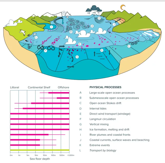
In this section, we will describe the different processes that govern the transport offloating plastics. These processes have been summarised infigure1, in which we have schematically depicted where in the ocean these processes are most relevant, from the littoral zone to the open ocean. Transport here is defined loosely as any movement of plastic particles from one location to another in three-dimensional space. When modelling this transport, it is typically decomposed into a deterministic and a stochastic component, the latter accounting for(turbulent) mixing processes that
Figure 1. Schematic of the physical processes that affect the transport of plastic(pink items) in the ocean (top panel). The table (lower panel) identifies in which regions different processes are important. Thick pink lines in the table mean that the process is among the most important in that water depth, while thin pink lines mean that the process is only of secondary importance. Transport by organisms is not a physical process and therefore represented with a green line instead of a pink one.
result from the unresolved part of the ocean currents, including wind and wave forcingfields varying ran-domly in space and time. Because of this stochastic component, it is more convenient in most cases to study particle transport with a large ensemble of plastic particles. Here, this ensemble transport is referred to as dispersion.
4.1. Large-scale open ocean processes
The horizontal large-scale flow is the most efficient way of transporting debris over large distances on the global scale, allowing connections between ecoregions and transport across basins. It is also the scale on which we know most about transport of floating plastics, partly because the Global Drifter Program that has been operational since the late 1970s is designed to measure this(Elipot et al2016).
Large-scale physical oceanography is built upon geophysical fluid dynamics (Pedlosky 1987, Val-lis 2006), a foundational theory well supported by
ocean observations since the early 20th century. For the purposes of this review, large-scale circulation is driven by surface winds, generating so-called Ekman drift at the sea surface under the influence of the Earth’s rotation, which is directed to the right of the wind in the Northern Hemisphere and to the left in the Southern Hemisphere. Ekman transport, integrated over the upper 10s of meters, creates regions of surface convergence and divergence, which in turn drive the large-scale geostrophicflow in the ocean interior. These areas of convergence are, on the large scale, found in all five subtropical gyres, which are basin-scale current sys-tems defined by wind stress patterns and coastal bound-aries(figure2). Surface divergence, on the other hand, is
found in the subpolar gyres and over parts of the South-ern Ocean. Floating plastic items that do not experience waves (see section4.4) or wind (see section 4.6) are
transported by surface currents and will accumulate in areas where surface waters converge. In contrast, areas of divergence (outside of subtropical gyres) typically have lower concentrations of floating plastic
(e.g. Maximenko et al 2012, Law et al 2014). In the
basin-scale convergence regions, the surface water is pumped down (so-called Ekman downwelling) to depths of a few hundred meters. However, the down-ward vertical velocity of the water near the surface is typically much smaller(10 s of meters per year) than the rise velocity of buoyant plastic(Reisser et al2015, Pou-lain et al2019), so that the floating plastic stays behind.
This Ekman/geostrophy theory is remarkably cap-able of predicting the large-scale distribution of float-ing microplastic in the ocean(Kubota1994, Martinez et al2009, Onink et al2019). This distribution reveals
large-scale accumulation of plastics in the centres of the subtropical gyres in areas termed ‘garbage pat-ches’. Despite a persistent, common misconception of a ‘garbage patch’ as a giant floating island of trash (which do not exist), concentrations there are still fairly low. Based onfield observations across the five subtropical gyres(Cózar et al2014, Eriksen et al2014, Law et al2010,2014), Cózar et al (2015) provided a
more accurate description of the‘garbage patch’, as large accumulation zones (millions of km2 in area) dominated by tiny plastic pieces mainly on the order of millimeters, not easily perceptible by an observer on a ship. When the sea is calm, these plastic particles are present in nearly 100% of net surface tows in these areas, each covering around 1000 m2, but the density of plastic pieces is not as high as the term‘patch’ may suggest. The typical mean spatial concentration mea-sured with net tows is around 1 plastic item in 4 m2, reaching 1–10 items m−2in the most polluted area. The accumulation zones in the subtropical gyres show high heterogeneity at multiple scales(e.g. Goldstein et al2012, Brach et al2018), and their borders are
dif-fuse and changing. The gyres are not stationary in space nor static in time. Rather, the gyres, and with them the accumulation zones, change shape and move with time(Howell et al2012, Lebreton et al2018), and
plastics are not trapped indefinitely in these gyres (van Sebille et al2012a, Maes et al2016).
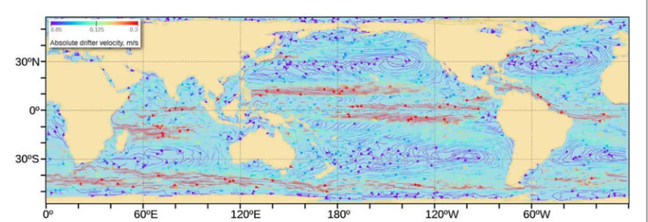
Figure 2. Schematic of large-scale ocean surface currents(gyres, convergence zones) based on mean velocities of undrogued surface drifters, with colouring indicative of speed. Floating plastic has been predicted and measured to accumulate in the centres of thefive subtropical gyres, which can be seen in thefigure as the points around which the drifters circulate centred at 30 degrees latitude in both hemispheres.
While the large-scale open ocean processes can reasonably well explain the observed debris pattern (with some notable exceptions, e.g. in the North Atlantic accumulation zone, see also van Sebille et al (2015b), it is important to realise that these theories do
not make any statements about the pathways and time scales of real plastic particles from sources into the open ocean accumulation zones. Furthermore, the vertical structure of near-surface currents(upper 10 s of meters, see also sections4.4,4.7and4.8) appears to
have a considerable impact on the large-scale circula-tion patterns(Wichmann et al2019), especially in the
Indian and South Indian Oceans, where van der Mheen et al(2019) found that drifters drogued at 15 m
depth give different accumulation patterns than undrogued drifters(see also Poulain et al2009, Lump-kin et al2012).
4.2. Mesoscale open ocean processes
Across the basin-scale gyre patterns, the ocean is full of eddies. Mesoscale eddies are slowly rotating vortices, with diameters of hundreds of kilometers(technically defined by the scale at which the Rossby number (e.g. Pedlosky1987) is much less than order one), depths of
few hundreds to thousands of meters and lifespans of weeks to years(Chelton et al2011). Mesoscale eddies
also form fronts and filaments between them by straining the surface waters; these fronts andfilaments become unstable and in turn form submesoscale eddies, which are smaller and faster evolving than mesoscale eddies(1–10 km diameter, with lifetimes of days to weeks). Eddies exist in two types: cyclonic eddies (rotating counter-clockwise in the Northern Hemisphere, and clockwise in the Southern Hemi-sphere), for which the radial component of the surface flow is mostly outward; and anticyclonic, for which the radial component is mostly inward(note that the same is true for gyres, explaining the above conv-ergence in anticyclonic subtropical gyres, and the divergence in cyclonic subpolar gyres). This inward surfaceflow for anticyclones could explain the obser-vation that an anticyclonic eddy had more floating debris in its core than a cyclonic one(Brach et al2018),
although submesoscale eddies are more effective in accumulating debris(see section4.3).
Nevertheless, the mesoscale eddies are certainly important, not only because they can retain debris, but also because the westward drift of these potentially long-lived structures can result in transport over thou-sands of kilometers, as has been shown for surface drifters(Dong et al2011), as well as radioactive isotope
markers (Budyansky et al 2015), plankton, jellyfish
(Johnson et al2005, Berline et al2013), heat and salt
(Dong et al2014). The explicit consideration of
mesos-cale eddy variability has, for example, shown a con-vergent pathway of seawater connecting the South Indian subtropical region with the convergence zone of the South Pacific through the Great Australian
Bight, the Tasman Sea, and the southwest Pacific Ocean(Maes et al2018), as well as into the Atlantic
Ocean via the Agulhas leakage(e.g. Beal et al2011, van Sebille et al2011).
Quasi-permanent jet-like features, commonly referred to as striations(Maximenko et al2008, Bel-madani et al2017), may also play a role in the transport
offloating plastics. Such small-scale structures are able to modulate the transport of surface material from the core of the convergence subtropical zones, revealing possible exit routes(Maes et al2016). Such long
dis-tance pathways of dispersion represent a challenge for ocean modelling, and the exact role of mesoscale and submesoscale processes, as well as the relative impor-tance of these processes in different ocean basins, are still not well known.
4.3. Submesoscale open ocean processes
In the last few decades, there has been increasing interest in oceanographic processes on scales smaller than a few tens of kilometers. Much progress has been made on describing, quantifying and developing a theory for these submesoscale features(Fox-Kemper et al 2011, Thomas et al 2013, McWilliams 2016).
These submesoscale processes are known to be very important locally for drifters and Sargassum accumu-lation(Szekielda et al2010, Pearson et al2019), as well
as oil spills transport and dispersion (Zhong and Bracco2013), as they systematically increase mixing
(Poje et al2014, McWilliams2019).
Particularly relevant to howfloating plastic parti-cles are affected by submesoscale processes was the finding in D’Asaro et al (2018) that flotsam
accumu-lates at density fronts and in cyclonic vortices (as opposed to the anticyclonic mesoscale eddies). The mechanism that causes this accumulation in cyclonic vortices is complicated, but is related to vortex stretch-ing of the submesoscale vortices. In eddies, the fronto-genesis and secondary radial-overturning circulation that cause surface convergence depend on the Rossby number. These processes are considerably stronger at the submesoscale than at the mesoscale for the same level of kinetic energy per unit area(e.g. Rascle et al
2017). Although often revealed from high-resolution
satellite imagery (e.g. Kudryavtsev et al 2012), these
submesoscale processes are typically not resolved even in‘high-resolution’ models.
4.4. Open ocean Stokes drift
During its periodic motion, a particlefloating on the free surface of a surface gravity wave experiences a net drift velocity in the direction of wave propagation, known as the Stokes drift (Stokes 1847). More
generally, the Stokes drift velocity is the difference between the average Lagrangianflow velocity of a fluid parcel and the average Eulerianflow velocity of the fluid (see van den Bremer and Breivik (2018) for a
reference frame, whereas in the Eulerian framework fluid motion is described at fixed spatial locations. Stokes drift arises due to the fact that particles subject to a surface wavefield move forward at the top of their orbits faster than backward at the bottom and spend longer in crests where their velocity is positive than in troughs where their velocity is negative.
Surface gravity waves on the open ocean are mostly caused by winds. For this reason, it is often assumed that any net transport carried by waves can be para-meterised as a fraction of the wind speed in the same direction as the wind(Weber1983). However, waves
are slower to build to strength and are more persistent than winds, and, once they have evolved into swell waves, they can travel long distances with low dissipa-tion(Ardhuin et al2009a, Hanley et al2010, Webb and Fox-Kemper 2015). Thus, the waves at a particular
location and time may have been caused by earlier winds at another location. Wave models, such as WAM and WaveWatch-III (Tolman 2009), were
developed to predict the propagation and strength of waves, and can therefore be used to predict Stokes drift.
Even though Stokes drift is a second-order effect (in the generally small steepness of the waves), whose magnitude is much less than the magnitude of the wave orbital motions themselves, the magnitude of the Stokes drift is frequently significant (McWilliams and Restrepo 1999). Either empirical wave spectra for
fully-developed waves(Pierson and Moskowitz1964, Hasselmann et al1976) or the output of wave models
can be used to accurately predict the Stokes drift (Webb and Fox-Kemper 2011, 2015) under the
assumption of weak surface slope. The simplification of monochromatic waves at the peak wave period, commonly adopted in Eulerian ocean models, leads to a Stokes drift that decays exponentially with depth, although alternative parameterisations have been pro-posed that more accurately capture the depth profile for realistic spectra(Breivik et al2016). For realistic
waves, the Stokes drift is strongly surface-intensified, decaying faster than exponentially for a typical spec-trum(Webb and Fox-Kemper2011,2015). From an
observational perspective, Stokes drift can be inferred from high-frequency radar(Ardhuin et al2009b) and
has the potential to be estimated from satellite mea-surements(Ardhuin et al2019). It can be accurately
measured in the laboratory(e.g. van den Bremer et al
2019).
Whetherfloating marine plastic particles are actu-ally transported with the velocity of their surrounding Lagrangianflow (and thus with the Stokes drift) and whether particles of all shapes, densities and sizes are transported at the same speed under similar condi-tions remain open quescondi-tions. Objects that are sub-merged, small and of the same density as the surroundingfluid will travel with the Lagrangian flow (Maxey and Riley1983). For fully submerged particles
that have a different density from the surrounding
fluid, it has been shown (Eames2008, Santamaria et al
2013) that their inertia can cause lighter (and thus
upward settling) particles to be transported more rapidly than the Stokes drift of the surroundingfluid and vice versa for heavier(downward settling) parti-cles. Furthermore, the response of particles to eddies and turbulence may also be different (Maxey and Riley1983). The shape of the particles determines their
orientation under waves but not necessarily their transport velocity(DiBenedetto and Ouellette2018).
For very steep waves, particles may surf on the wave (Pizzo2017) or be subject to transport faster than the
Stokes drift due to wave breaking(Pizzo et al2019).
Floating objects are subject not only to Stokes drift but also to motions with longer time scales(e.g. geos-trophic flow), as well as windage (see section 4.6).
Observations of these different transports indepen-dently are rare(e.g. Ardhuin et al2009a). Despite the
poorly understood complexity in the relationship between Stokes drift and transport of floating mat-erial, Stokes drift is one of the key components of many simulations of the drift offloating marine plastic particles. Different authors have considered its effects on different types of objects: for example, Stokes drift can make a significant contribution to the trajectories of drifters(Röhrs et al2012, Meyerjürgens et al2019);
it must be accounted for in search and recovery mis-sions(e.g. the crashed airplane MH370; Trinanes et al
2016, Durgadoo et al2019); and it can be key in the
local modelling of oil spills (Christensen and Ter-rile2009, Drivdal et al2014). In addition to transport,
a random wavefield and its associated random Stokes driftfield have the capacity to disperse or ‘diffuse’ a cloud of floating tracers (Herterich and Hassel-mann1982), but this effect is generally small, local and
dominated by other sources of dispersion(Herterich and Hasselmann1982, Spydell et al2007).
In an early study focusing on debris accumulation near Hawaii, Kubota(1994) found that Stokes drift did
not significantly contribute to debris transport, but only took into account Stokes drift derived directly from the local windfields and not swell. A number of recent modelling studies took into account Stokes drift from the entire wavefield, combining wind and swell waves, and found a greater role for Stokes drift. In the Sea of Japan, Stokes drift moved plastic particles between 5 and 10 mm towards the Japanese coast dur-ing winter (Iwasaki et al2017). A similar effect was
found in the Norwegian Sea (Delandmeter and van Sebille 2019). Stokes drift can also lead to leakage of
particles out of the Indian Ocean(Dobler et al2019)
and can cause drifting particles to cross the strong cir-cumpolar winds and currents and reach the Antarctic coast(Fraser et al2018). On a global scale, Stokes drift
does not per se contribute to large-scale accumulation of microplastics in the subtropics, but does lead to an increased transport to polar regions where storm-gen-erated waves are larger and occur more frequently (Onink et al2019).
As the Stokes drift depends strongly on the shape of the waves(it is proportional to the square of their steepness), rapid changes in the waves can lead to rapid changes in particle transport. This plays a role in the coastal zone, where waves steepen and ultimately break (see section 4.11), and during storms, when
waves rapidly steepen and the Stokes drift rapidly increases. This change is crucial for plastic debris beaching: developing steep stormy waves may‘grab’ plastics and sediments from the beach, and transport these offshore; whilst smoother waves, which remain after the wind ceases, slowly return plastics and sediments back to shore (Chubarenko and Stepanova2017).
Finally, it cannot be emphasized enough that the Stokes drift and the Eulerian currents do not evolve independently. Two effects need to be distinguished. First, a realistic ocean is not made up of regular waves, but the broad-banded spectral content of its waves leads to a group-like structure. For wave groups, the net positive transport associated with the Stokes drift becomes divergent on the group scale and is accom-panied by an opposing Eulerian returnflow at depth (Longuet-Higgins and Stewart 1962, Haney and Young2017). In the open ocean, this return flow is
very small and will not have any significant effect on the transport offloating plastics (van den Bremer and Taylor2016).
Second, there are important connections between the Stokes drift and the Eulerian currents through the Stokes forces (Hasselmann 1970, Craik and Leibo-vich1976, McWilliams et al1997, Ardhuin et al2007, Lane et al2007, Polton and Belcher2007, Suzuki et al
2016). While the dynamical details of these
interac-tions exceed the goals of this paper, it is sufficient to note that, at leading order, there is often an important anti-Stokes response of the Eulerian current to the pre-sence of Stokes drift, and such an anti-Stokesflow has been observed in situ in coastal areas(Lentz and Few-ings 2012). This tendency for the Eulerian flow to
oppose the Stokes current is caused by the Stokes for-ces that connect the Stokes drift to the Eulerian cur-rents, primarily the Stokes-Coriolis and Stokes advection terms. If these forces are unbalanced, then effectively a net force from the waves is applied to the Eulerian currents until they oppose the Stokes drift. This effect recasts the standard large-scale geophysical fluid dynamics problems to include Stokes effects: wavy Ekman layers (McWilliams et al 2012), wavy
geostrophic fronts and filaments (McWilliams and Fox-Kemper2013), and wavy hydrodynamic
instabil-ities (Haney et al 2015). On large scales, the
con-sequence is that the net Lagrangian transport (combining the Stokes and Eulerian currents) behaves much like the traditional large-scale transport theory predicts: Ekman layers and geostrophic currents dri-ven by Ekman convergence. The anti-Stokes response explains how Stokes advection by itself can cause a lar-ger impact than Stokes advection plus other Stokes
forces(Breivik et al2015). On the mesoscale and
sub-mesoscale, the Stokes vortex and Stokes shear forces become important (McWilliams and Fox-Kem-per2013, Suzuki and Fox-Kemper2016), which can
influence frontogenesis, instabilities, and turbulence (Haney et al2015, Suzuki et al2016) and indeed leads
to a further reinforcement of the anti-Stokes effect (Pearson2017). On smaller scales, the Stokes vortex
and shear forces play a major role and lead to Lang-muir circulations and LangLang-muir turbulence.
In regards to the transport of plastics and other pollutants by Stokes drift, one must be careful to con-sider the forces of interaction between the Stokes and Eulerian flows. In a modelling context, this means simultaneously solving a wave model and an ocean transport model with the correct coupling between them. Models that explore this are e.g. COAWST (Warner et al2010), SWAN+ADCIRC (Dietrich et al 2012) and UWIN-CM (Curcic et al2016, Li et al2018).
Exploring the consequences of such coupled model-ling for the transport of marine debris will be one of the most important challenges ahead.
4.5. Internal tides
The movement of the tides over banks, reefs, and the continental shelf break generates large internal waves generated by internal tides (Kao et al 1985, Hibiya1990). Surface convergences moving with these
waves have been demonstrated to concentrate and transport larval invertebrates,fish and tar balls from an oil spill (Shanks 1983, 1987, 1988). The most
common site for the generation of these internal waves is the continental shelf break. As the tide ebbs off the shelf, a lee wave or hydraulic jump is produced over the continental slope. When the tide changes toflood, this lee wave propagates up onto the shelf and shoreward where it evolves into a train of internal waves. As the waves move into shallow water they can break forming an internal (underwater) bore (Cairns1967, Winant1974, Pineda1995).
Surface currents are generated over the internal waves(Shanks1995). Over waves of depression (the
nonlinear wave has a trough but no crest), the surface current is in the direction of wave propagation. At the surface over the leading edge of the wave, the surface current turns downward forming a surface conv-ergence, which moves along with the wave. Over larger waves of depression the surface current can be as fast or faster than wave propagation and, under these con-ditions, objects at the surface, for example surface-oriented larvae or buoyantflotsam, are carried into the convergence, concentrated there and transported along with the internal wave(Shanks et al2000).
Waves generated at the shelf break may cause transport across the shelf. Where waves are generated over a bank, they can propagate over deep water for long distances, e.g. large internal waves are generated over the Pearl Bank in the Sulu Sea and propagate
across the basin hitting the coast of Palawan Island (Apel et al1985). In the Caribbean, internal waves are
formed around Trinidad and Tobago and propagate northward(Giese et al1990). In the Mediterranean,
they are formed over the Camarinal Sill at the Strait of Gibraltar(Bruno et al2002).
Convergences over sets of internal waves are visi-ble from space in both visivisi-ble and synthetic aperture radar (SAR) images (Apel et al 1975, Alpers1985).
When winds are light, convergences appear as slicks of smooth water; oils in the surfacefilm are transported into the convergence dampening capillary waves. Often floating material, algae and flotsam, become concentrated and transported along with the waves. Each wave of a set can generate a surface slick. Similar to surface waves, tidally generated internal waves are refracted by the bottom topography; hence, the sur-face slicks tend to be oriented parallel to bottom con-tours. Sailing perpendicular to a set of waves, convergence zones appear as long (100s of meters) slicks oriented parallel to the bottom contours with distances separating the slicks on the order of 100s of meters. The edges of the slicks are sharply delineated. This set of features is characteristic of tidally generated internal waves and can be used as a diagnostic tool to identify their surface expression(Shanks1983).
4.6. Transport due to direct wind force(windage) Windage is the effect of wind on items with a freeboard, i.e. an area protruding out of the water. While the wind-induced displacement velocity may be directly related to the wind speed(Tapia et al2004, Astudillo et al2009), it is important to realise that
windage does not correspond to the portion of surface flow field driven by the wind, which is already contained in the surface current, but to the direct wind drag exerted on items at the sea surface(Zambianchi et al 2014). In practice, the effects of windage and
Stokes drift(at least that of the locally wind-driven waves) are typically combined, and the so-called ‘leeway’ is defined as the wind and wave-induced motion of a drifting object relative to the ambient current (Richardson1997, Kako et al 2010, Breivik et al2011).
Ignoring its Stokes drift component, windage results from the combination of a skin drag and a form drag forces (e.g. Petty et al2017). Skin drag results
from the viscous friction on the surface of the object exposed to the wind. Form drag arises because of the wind pressure on the part of the object above the sea surface. The latter depends quantitatively on the buoy-ancy ratio (the ratio between the cross-sections of floating objects normal to the wind direction above and below the sea surface), which in turn depends on both the density and shape of afloating body (Zam-bianchi et al2014, Ryan2015). This aspect may be very
relevant for floating marine debris, as it might be responsible for sorting plastics with different
buoyancies and sizes. This affects their wind drag coef-ficient (Chubarenko et al2016, Pereiro et al2018) and
hence their dispersion(Aliani and Molcard2003),
ulti-mately affecting both residence time and beaching characteristics of floating items (Yoon et al 2010).
Model simulations of Maximenko et al(2018) of
drift-ing debris generated by the 2011 tsunami in Japan have been validated using observational reports, and demonstrated that‘high-windage’ objects crossed the North Pacific in less than a year and were relatively quickly pushed from the ocean onto the North Amer-ican coastline, while heavy, low-windage debris col-lected in the mid-basin convergence zone.
4.7. Langmuir circulation
In some circumstances, the surfaceflow can attain the form of coherent roll structures: pairs of counter-rotating vortices aligned horizontally. The most well-knownflow of this type is the Langmuir circulation (Langmuir 1938), which can be recognised by the
formation of windrows.
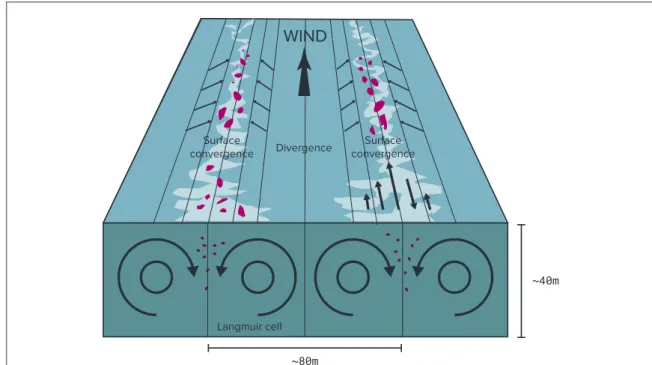
Windrows are common and clearly identifiable features of the surface ocean. They are lines of bubbles and surface debris generally aligned with the wind that are the visible surface manifestation of the conv-ergence zones between wind-wave-induced, counter-rotating, wind-parallel helical vortex pairs referred to as Langmuir circulation(figure3). Planktonic
organ-isms also accumulate in Langmuir circulation cells, potentially enhancing the biofouling of flotsam, as well as increasing the likelihood of accidental entan-glement in, and ingestion of, plastic items by more mobile predators due to the close proximity between plastic and biota(Gove et al2019).
The formation of Langmuir cells is the manifesta-tion of the interacmanifesta-tion between the wind-induced shear flow and the wave-induced Stokes drift (Craik1977, Leibovich1977,1980). It can be shown
mathematically that shearflow becomes unstable in the presence of vertically sheared Stokes drift. Small perturbations in the downwindflow lead to the forma-tion of downwind-directed rolls, so that water parcels describe spiral trajectories. Langmuir circulation cells generally occur under wind speeds greater than 3–5 m s−1, and their formation and/or re-formation takes only about a few minutes(Thorpe 2004). Alternate
cells, which can be kilometers long, rotate in opposite directions, causing formation of lines with converging and diverging surface flows associated with down-welling and updown-welling, respectively, beneath these lines. The water in the cells also moves downwind, so that motion is helical.
Convergence and divergence zones in Langmuir circulation are difficult to spot over the water surface (Faller1964), but become visible when there is foam or
flotsam on the surface accumulated by the conv-ergence. After only 15–20 min of wind action, floating material can already be accumulated in stripes, and is
kept there as long as the particular row persists(Chang et al 2019). Over time, the cells become larger and
merge together, leading to the formation of Y-junctions at the surface(Thorpe2004, Marmorino et al 2005), pointing generally down-wind in deep
waters or equally up- and down-wind in shallow areas (Chubarenko et al2010). The lifespan of Y-junctions is
only 2–5 min, after which the regular structure of windrows is re-established.
Even when windrows may not be apparent or are highly disordered, the vertical velocity magnitude of near-surface turbulence can be enhanced by the pre-sence of Stokes forces, a condition known as Langmuir turbulence(McWilliams et al1997, McWilliams and Sullivan2000, D’Asaro et al2014). Because of the close
connection between vertical velocities and surface convergence, the disordered windrows may still parti-cipate in the active accumulation of surface material on horizontal scales of 10s to 100s of meters(Carlson et al2018).
Langmuir circulations, submesoscale fronts, inter-nal waves, and other related roll-like instabilities with surface convergence (van Roekel et al 2012) may
explain occasional observations from ships of extre-mely high concentrations offloating debris ordered in 2–3 m wide stripes that stretch to the horizon (Faller1964, Barstow1983, Law et al 2014, Carlson et al2018). These parallel windrows were seen in the
centres of the gyres under low-wind conditions; how-ever, the exact census of the dynamics forming them is incomplete, and their frequency of occurrence is poorly constrained observationally. However, climate models that parameterise Langmuir turbulence and submesoscale fronts and eddies predict them to be
globally ubiquitous(Fox-Kemper et al2011, Li et al
2016).
The relatively strong vertical flows in Langmuir circulation may remove smaller items from the sur-face, especially when the buoyancy of plastic particles is small compared to the vertical current(Brunner et al
2015, Kukulka and Brunner2015). Observed vertical
profiles of microplastics concentrations are only con-sistent with turbulence-resolving simulations if Lang-muir circulation is explicitly included in the model (Brunner et al2015). Submesoscale structures, such as
strong fronts, can play a similar role(Smith et al2016, Suzuki et al2016, Taylor2018). Sampling of
micro-plastics from nets that only skim the surface may underestimate abundance in areas of divergence or overestimate in areas of convergence.
Non-neutrally buoyant particles(whether sinking or rising) in a laminar, near-surface flow will describe closed elliptic trajectories within a‘zone of retention’ under the water surface(Stommel1949), and the
com-bination of these coherent structures and turbulence will tend to homogenise the particles across the reten-tion zone(Farmer and Li1994). For positively buoyant
particles there are two qualitatively different beha-viours(Bees et al1998): some particles are trapped in
closed orbits at some distance below the surface(the Stommel retention zone), whereas others accumulate at the line of convergence at thefluid surface. In the absence of any other transport or diffusive processes, buoyant particles that begin at the surface cannot sub-merge and, hence, will not enter the Stommel reten-tion zone no matter how fast thefluid flow is in the Langmuir circulation. It is rare tofind such circum-stances, however, as waves and the occasional white-capping or breaker typically coexist with Langmuir
Figure 3. Schematic of Langmuir circulation and water dynamics therein. Pink particles are plastic particles, which accumulate in regions where Lagmuir cells converge at the surface. Adapted from Dethleff et al(2009).
turbulence. Analysis of forces(the buoyancy force and the dynamic pressure force) acting on particles (Deth-leff et al2009, Chubarenko et al2010), shows that
par-ticles recirculate, describing different retention trajectories depending on particle size and density(see also Woodcock 1993). Thus, Langmuir turbulence
inter-mixes particles near the surface of the ocean by forcing particles with different buoyancy to follow dif-ferent paths.
Stokes drift, Langmuir circulation, and the buoy-ancy of marine debris also influence the horizontal dispersion of buoyant material in the ocean surface layer(Colbo and Li1999, Kukulka and Veron2019).
Horizontal dispersion is driven by vertically sheared horizontal mean currents and turbulent velocities. Less buoyant material is mixed throughout the ocean boundary layer(which is about 10–100 m deep), so that dispersion by shear is predominant, whereas more surface-trapped (but still fully submerged) buoyant particles are dispersed by turbulent currents (Liang et al2018).
Realistic ocean models where Stokes drift has been included(Warner et al2010) show significant
improvements in regions where wave-current interac-tions are strong. On the other hand, Langmuir circula-tion and turbulence are not commonly included explicitly in regional or global ocean models, although recent software developments in GOTM(Umlauf and Burchard2003) and CVMix (Griffies et al2015) may
make using parameterisations of Langmuir turbulence easier(Li et al2019). In idealised settings, Langmuir
turbulence has led to improvements in parameterisa-tions of vertical mixing in the boundary layer (McWil-liams and Sullivan2000, Kantha and Clayson2004, Harcourt2012, Noh et al2015), which could form the
basis for stochastic parameterisations of three-dimen-sional transport of particles(e.g. Holm2015).
4.8. Vertical transport and mixing
The vertical distribution offloating plastic depends not only on the particle’s buoyancy, but also on the dynamic pressure due to vertical movements of ocean water. Understanding of the verticalflow in the ocean is challenging because it is induced by several processes acting at different temporal and spatial scales. It can exist as coherent structures such as large-scale (Ekman) pumping, upwelling and downwelling, fronts, and turbulence-induced roll structures such as convection cells and Langmuir circulations. Wave-enhanced turbulence is also present without large-scale features(e.g. Kukulka et al2012). There can also
be vertical mixing in estuaries and river mouths, but in the presence of strong stratifications and tidal motion, the vertical mixing of plastics is much more complex there(see sections4.10and4.11). The typical scales of
these processes in the open ocean are presented in table1, ranked from highest to lowest averaged vertical velocity.
Diurnal heating of the ocean surface layer also influences near-surface vertical mixing processes. Strong surface heatfluxes result in diurnal warm layers with near-surface density gradients (Price et al
1986, Soloviev and Lukas 1997, Plueddemann and Weller 1999). Such density stratification suppresses
turbulence and associated near-surface mixing(Li and Garrett1995, Min and Noh2004, Kukulka et al2013).
Turbulence-resolving large-eddy simulations indicate that turbulent downwardfluxes of buoyant tracers are suppressed in heating conditions, so that buoyant material is surface-trapped, which is consistent with microplastics observations in the Atlantic and Pacific Oceans(Kukulka et al2016).
Measured rise velocities for various types of plas-tics and size classes typically range in the order of milli-metres to 10s of centimilli-metres per second(Reisser et al
2015, Lebreton et al2018, Poulain et al2019), which
places the rise velocity right in the middle of the range of vertical velocities typical of boundary layer turbu-lence and the submesoscale(Taylor2018) in table1. It may also be important to take into account the effect of the positively-buoyant particles sized around the Kolmogorov micro-scale(Ruiz et al2004, Cózar et al
2014), and the dynamics of flow around suspended
particles(Maxey and Riley 1983). It is worth noting
here that the vertical dispersion of buoyant particles in the water column has been studied in the past, for example, in the context of frazil ice dynamics (Svens-son and Omstedt1998), algal blooms (Moreno-Ostos
et al2009), and diurnal vertical migrations, and that
lessons could be learned from these case studies. 4.9. Ice formation, melting and drift
The poleward migration offloating plastics from highly populated latitudes to polar regions has been reported in the Northeastern Atlantic sector of the Arctic Ocean (Lusher et al2015, Bergmann et al2016, Cózar et al
2017), and the central Arctic Ocean (Kanhai et al2018).
Once there,floating plastic takes part in the cycles of formation and melting of the sea ice. Observations show (Obbard et al 2014, Peeken et al 2018a,2018b) that
Arctic sea ice has microplastics concentrations that are several orders of magnitude higher than that in the water column. Sea ice has already been identified as a major means of transport and redistribution for sediments(Nürnberg et al1994, Gregory et al2002);
various pollutants and contaminants in polar regions (Pfirman et al1997, Rigor and Colony1997, Korsnes et al2002), including oil spills (Blanken et al2017); as
well as microplastics(Peeken et al2018b).
As with other particles, plastic particles become concentrated in sea ice during ice formation through a process known as scavenging(figure 4), which
con-centrates particles by 1–2 orders of magnitude relative to ambient seawater(Obbard et al2014). Even though
this phenomenon has not yet been investigated for plastics specifically, the details of the process probably
depend on the shape, size and density of plastic parti-cles. As ocean water cools to the freezing point(and slightly below it), small needle-like ice crystals form (typically 3 to 4 mm long; called frazil ice). These crys-tals consist of nearly pure freshwater, releasing salt into the surrounding sea water. At this stage, both thermal and haline convection develops in the upper water layer, sometimes to depths of several metres (Lake and Lewis1970, Ushio and Wakatsuchi1993, Peterson 2018). The frazil crystals are usually
sus-pended in the top few centimetres of the surface layer of the ocean, but can be stirred to a depth of several metres by wave-induced turbulence(Omstedt 1985, Svensson and Omstedt1998). With further cooling,
the growing number offloating frazil crystals aggre-gate and freeze together, leading to the formation of grease ice(a soupy layer on the surface), then slush and shuga(behaving like a layer of a viscous fluid, a few cm across), then nilas (elastic crusts up to 10 cm thick), then pancake ice(typically up to 10 cm in thickness, 30 cm–3 m in diameter). Brine releases during the growth of the ice, and vertical(thermal plus haline) convec-tion supports further mixing, transporting suspended particles to the upper water layers. This way, both floating and slightly-negatively buoyant plastic parti-cles could come into contact with newly-freezing ice needles and thus be captured into the ice.
In contrast to freezing, melting of sea ice takes place at the air-sea interface. This provides a certain ‘lifting’ mechanism for the (plastic) particles under freeze/thaw cycles: being captured by growing ice from below, they become closer to the surface as the ice melts.
Sea-ice can also transport plastic particles lat-erally. Therefore, sea-ice movements can be used to track the movement of trapped plastics(Peeken et al
2018b). Instruments such as passive microwave
satellite images combined with the motions of sea ice buoys have been used to study sea ice drift patterns (Tschudi et al 2010, Tekman et al 2017).
Under-standing these dynamics is especially important in the context of future trends towards thinner sea ice and ice-free summers, and changes in the extent of ice-free areas, ice movement patterns in polar regions and resulting changes in ocean circulation transport. Changes caused by the shift from multi-year ice extent tofirst-year ice might result in the ten-dency of sea icefloes to diverge from the main drift pattern such as the Transpolar Drift (Szanyi et al
2016), with complex effects on exchange processes of
any contaminants between the Exclusive Economic Zones of the various Arctic nations (Newton et al
2017).
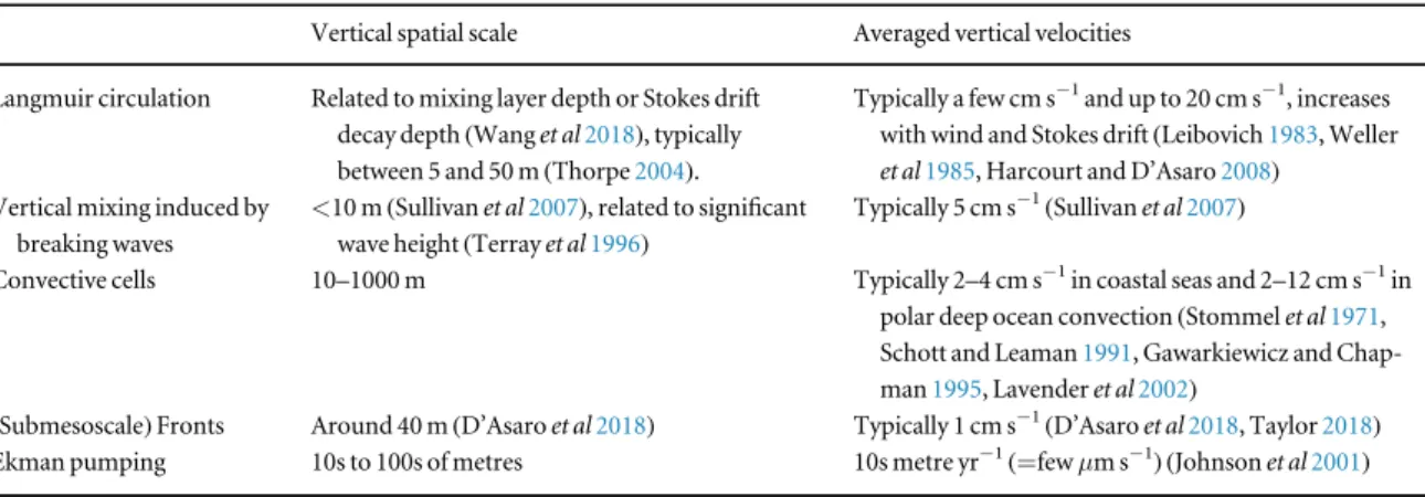
Table 1. Characteristic vertical spatial scales and averaged vertical velocities for different open ocean processes inducing vertical transport. Vertical spatial scale Averaged vertical velocities
Langmuir circulation Related to mixing layer depth or Stokes drift decay depth(Wang et al2018), typically
between 5 and 50 m(Thorpe2004).
Typically a few cm s−1and up to 20 cm s−1, increases with wind and Stokes drift(Leibovich1983, Weller et al1985, Harcourt and D’Asaro2008)
Vertical mixing induced by breaking waves
<10 m (Sullivan et al2007), related to significant
wave height(Terray et al1996)
Typically 5 cm s−1(Sullivan et al2007)
Convective cells 10–1000 m Typically 2–4 cm s−1in coastal seas and 2–12 cm s−1in polar deep ocean convection(Stommel et al1971, Schott and Leaman1991, Gawarkiewicz and Chap-man1995, Lavender et al2002)
(Submesoscale) Fronts Around 40 m(D’Asaro et al2018) Typically 1 cm s−1(D’Asaro et al2018, Taylor2018)
Ekman pumping 10s to 100s of metres 10s metre yr−1(=few μm s−1) (Johnson et al2001)
4.10. River plumes and coastal fronts
Large rivers can move plastic debris originating on land out to sea (Lebreton et al2017, Schmidt et al
2017). In (sub-)polar regions, this can be exacerbated
seasonally by melting of riverine ice in spring, carrying previously ice-locked plastics to sea (Holmes et al
2012). In river plumes, the river water and ocean water
are in direct contact, forming fronts that may persist for 10s or 100s of kilometres into the open ocean. Plume fronts are often visible from large distances (including from space) due to the contrasting optical properties of these water masses(Acha et al2015). At
estuarine fronts, distinct differences between the water masses can be observed, typically with the lighter freshwater at the surface extending farther out to sea, and the denser seawater below intruding farther upriver.
Floating objects(both natural and anthropogenic) tend to accumulate at these fronts for similar reasons as for the submesoscale frontogenesis processes described above, which is reflected in higher debris abundance along the outer river plume edge(Atwood et al2019), as well as on the seafloor and on the shore
(Acha et al2003). River plumes may also contribute to
the accumulation of floating debris on seashores downstream of contaminated rivers. Microplastic beaching rates have been shown to depend strongly on the characteristics of the river mouth(Atwood et al
2019), and seashores downstream of the river outflow
had higher densities of anthropogenic debris than sea-shores upstream or distant from river mouths(Rech et al2014, Cheung et al2016). Finally, coastal fronts,
whether generated by river plumes, upwellings, or by other processes, may also block the transport of float-ing items, includfloat-ing marine plastics(Hinojosa et al
2011, Garden et al2014, Ourmieres et al2018). As has
been shown for sediments, nutrients and Persistent Organic Pollutants(POPs), river mouths and coastal zones can act as physico-chemical barriers, orfilters, retaining and modifying a certain part of theflux of the material towards the ocean (e.g. Emelyanov 2005).
Enhancedflocculation of clay and organic matter in areas of contact of riverine and marine waters may also favour the retention offloating plastic objects.
4.11. Coastal currents, surface waves and beaching The dominant hydrodynamics in coastal waters that control the transport of plastic particles differ signi fi-cantly from the hydrodynamics occurring in the open ocean. The complex 3D circulation patterns control-ling plastic transport on the onshore side of the inner shelf region are largely influenced by wind, waves and tides, with the relative importance of forcing depend-ing on water depth(Lentz and Fewings2012). Tidal
currents generate turbulence near the bottom (Trow-bridge and Lentz2018). In estuaries, tides and density
fields also interact in complex ways, for example resulting in converging fronts or particle trapping
(MacCready and Geyer2010). The coastline
morph-ology and its interaction with the hydrodynamics also impact particle transport and, due to the shallowness of the water, even horizontal transport of floating plastics is influenced by the seafloor.
The presence of the seabed results in a substantial nonlinear evolution of the waves from their deep-water state(Elgar and Guza1985). The shape of
indivi-dual shoaling waves changes from an almost symme-trical profile in deep water to a shape with sharp crests and broad, flat troughs in coastal waters (Elgar and Guza1985, Doering and Bowen1995). This increase
in steepness has important implications for the strength of the Stokes drift(see section4.4).
Further-more, as ocean surface gravity waves move from off-shore regions to coastal waters, they start to feel the seabed and some of the wave energy is dissipated by friction, resulting in a thin boundary layer. Within this layer, the horizontal and vertical orbital velocities are not exactlyπ/2 out of phase, resulting in a net hor-izontal wave Reynolds stress acting in the direction of wave propagation, known as boundary layer stream-ing(Longuet-Higgins1953), which acts in addition to
the Stokes drift.
The wave asymmetry increases until the waves become unstable and eventually break. Wave breaking enhances the Lagrangian drift close to the surface (Deike et al2017, Pizzo et al2019). The enhanced
tur-bulence due to wave breaking increases mixing, which can cause resuspension of particles from the seabed (Deigaard1993). Broken waves propagate further in
the inner surf zone until they reach the shoreline, where they collapse and climb up and down the beach face in the swash zone. The transport of plastic in the swash zone depends on plastic buoyancy and swash zoneflow asymmetry (Hinata et al2017). Large
float-ing particles that are seaward of the shoreline but within a distance of approximately half of the run-up length are susceptible to beaching(Baldock et al2008).
Particles with low settling velocity are recaptured by small eddies(with diameters of centimeters to meters) induced by swash waves and then transported sea-ward, while large particles with high settling velocities remain in the swash region(Hinata et al2017). This
obviously has impacts on the residence time of plastic close to the beach face. Plastic particles washed ashore by large waves will deteriorate at rates that depend on weathering history and residence time on the beach, and fragment into small pieces that can be backwashed offshore by swash waves and wave-induced nearshore currents(Isobe et al2014, Kataoka and Hinata2015).
The wave evolution and dissipation also induces currents, which are three-dimensional, and their influence can be separated into a cross-shore component (perpendicular to the coastline) and a longshore component (parallel to the coastline). Waves approaching the coastline at an angle result in a net longshore current that moves particles along the coast(Longuet-Higgins and Stewart1962, Taffs and
Cullen 2005). In the cross-shore direction, an
off-shore-directed mean velocity, termed the mean return flow or undertow, exists within the surf zone as a result of a vertical imbalance between the wave-induced momentum flux (radiation stress) and the pressure gradient generated by the mean water surface slope (Svendsen1984).
Buoyant plastic particles are affected more by the onshore drift as they have a tendency to remain at the sea surface, whereas small plastic particles are more likely to be mixed into the water column and follow the undertow offshore(Isobe et al2014, Kataoka and Hinata2015). As evidence of this, more floating plastic
bottles were found inside the surfzone than outside it in an observational survey in the southern Mediterra-nean(Pasternak et al2018). Other studies describing
zooplankton accumulation have also reported a corre-lation between the position of the plankton commu-nity in the water column with onshore transport due to surface Stokes drift or bottom streaming and off-shore transport in the mid-water-column undertow (Shanks et al2015). Furthermore, because of this
ver-tical variation in the horizontal mean velocity, beach morphology influences the direction of transport: more dissipative beaches tend to trap plankton inside the surf zone, while reflective beaches keep the plank-ton outside the surf zone(Morgan et al2017).
A particularly relevant wave-induced current is the rip-current, which is a seaward-directed current that originates within the surf zone, expands outside the breaking region and can extend to the inner shelf(see figure5). Rip-currents eject surf zone water onto the
inner shelf and are potentially an important channel for seaward transport of plastic particles. Rip-current systems can trapfloating material within the surf zone, as the surf zone currents move particles toward the centre of the rip(MacMahan et al2010, Fujimura et al
2014).
There is still surprisingly little literature on the processes that control how plastic and other buoyant pollutants, such as oil, beach. Attempts have been made to create data-driven estimates of litter on bea-ches, where beach litter categories are predicted over time using artificial neural networks, using data of large debris on beaches from cleanup surveys (e.g. Balas et al2004, Schulz and Matthies2014, Granado et al2019). Another approach is based on the fact that
natural sorting and retention of certain type of sedi-ments(sand, granules, pebbles) are observed on coast-lines (Reniers et al 2013). The same could be
happening with plastic particles: beach characteristics like steepness and sediment type could determine which particles get stranded(Hardesty et al 2017b).
For example, surface roughness and the pore size of the beach sediments are likely to be important when plastic objects are pushed on the shore by the wave run-up.
Finally, coastlines are also considered to be hot-spots for microplastic generation (Andrady 2011).
Degradation of plastic appears to be related to ultra-violet radiation and/or mechanical abrasion by sedi-ments(Song et al2017) and fragmentation in the sea
swash and wave breaking zone, especially during storm events(Chubarenko and Stepanova2017, Chu-barenko et al2018, Efimova et al2018). The
fragmen-tation rate of beached plastic might be closely related to the residence time on beaches (Kataoka and Hinata2015, Fanini and Bozzeda2018) and is
depen-dent on polymer type(Song et al2017) and
temper-ature(Andrady2011).
4.12. Extreme events
While extreme events such as floods, tsunamis and storms are known to play an important role in the release of plastic and other materials into the ocean