En vue de l'obtention du
DOCTORAT DE L'UNIVERSITÉ DE TOULOUSE
Délivré par :
Institut National Polytechnique de Toulouse (INP Toulouse) Discipline ou spécialité :
Intelligence Artificielle
Présentée et soutenue par :
M. CLÉMENT CARBONNEL
le mercredi 7 décembre 2016
Titre :
Unité de recherche : Ecole doctorale :
Harnessing tractability in constraint satisfaction problems
Mathématiques, Informatique, Télécommunications de Toulouse (MITT)
Institut de Recherche en Informatique de Toulouse (I.R.I.T.) Directeur(s) de Thèse :
M. MARTIN COOPER M. EMMANUEL HEBRARD
Rapporteurs :
M. STANISLAV ZIVNY, UNIVERSITY OF OXFORD M. STEFAN SZEIDER, WIEN UNIVERSITAT
Membre(s) du jury :
1 Mme NADIA CREIGNOU, AIX-MARSEILLE UNIVERSITE, Président
2 M. EMMANUEL HEBRARD, LAAS TOULOUSE, Membre
2 M. MARTIN COOPER, UNIVERSITE PAUL SABATIER, Membre
First and foremost, I would like to thank my supervisor Emmanuel Hebrard. Emmanuel was always there to guide me, answer my questions, comment on my re-search and support me in the difficult moments; he really took his supervision role to heart and worked hard to ensure I do my Ph.D. in the best possible conditions. Through countless discussions, he has shaped my scientific mind and prepared me for the world of academic research. It has been a pleasure and an honour working with him.
I would also like to thank my co-supervisor Martin C. Cooper for his invalu-able scientific advice and the opportunities he gave me. His numerous and detailed comments on my ideas and manuscripts have been of great help.
I thank the members of the ROC team at LAAS-CNRS for these three years spent together. It was a great experience, both from the scientific and personal point of view. I am particularly indebted to Christian Artigues, who battled to obtain funding and make this thesis happen.
I thank every person who took the time to read my manuscript, including my referees Stanislav ˇZivn´y and Stefan Szeider as well as the other members of my committee, Nadia Creignou and Philippe J´egou.
I thank those who have played a role (sometimes indirectly) in shaping the path that ultimately led me to write this dissertation - that includes among others Gilles Trombettoni, Philippe Vismara and many of my teachers and friends from Lyc´ee Champollion, Ensimag and Universit´e Joseph Fourier.
Contents
1 Introduction 7
2 Background 11
2.1 Constraint Satisfaction Problems . . . 12
2.2 Language-based Tractable Classes . . . 15
2.2.1 Expressive Power of Constraint Languages . . . 16
2.2.2 Polymorphisms . . . 17
2.2.3 Tractability via Local Consistency . . . 20
2.2.4 Tractability via Few Subpowers . . . 23
2.3 Structural Tractable Classes . . . 24
2.4 Parameterized Complexity . . . 26
3 Backdoors into Tractable Constraint Languages 31 3.1 Strong Backdoors . . . 32
3.2 Composite Classes . . . 35
3.3 Complexity of Strong Backdoor Detection . . . 38
3.3.1 Parameter k . . . 40
3.3.2 Combined Parameter k+r . . . 42
3.3.3 Constant-closed Classes . . . 50
3.4 Partition Backdoors . . . 53
3.5 Preliminary Experiments . . . 55
3.6 Conclusion and Future Research . . . 57
4 Meta-Problems in Conservative Constraint Satisfaction 59 4.1 Meta-Problems . . . 61
4.2 Conservative Constraint Satisfaction . . . 62
4.3 Tools . . . 64
4.4 Semiuniform algorithms . . . 67
4.5 Semiuniformity and Conservative Polymorphisms . . . 68
4.6 Deciding the Conservative Dichotomy in Polynomial Time . . . 73
4.7.1 Conservative Mal’tsev Polymorphisms . . . 78
4.7.2 Conservative Majority Polymorphisms . . . 83
4.8 Conclusion and Future Research . . . 85
5 Kernel-based Propagators: the Vertex Cover Constraint 87 5.1 Loss-less Kernels . . . 88
5.2 Vertex Cover . . . 93
5.2.1 Preliminaries: Classical Kernelization . . . 94
5.2.2 z-loss-less Kernels for Vertex Cover . . . 96
5.2.3 The VertexCover Constraint . . . 99
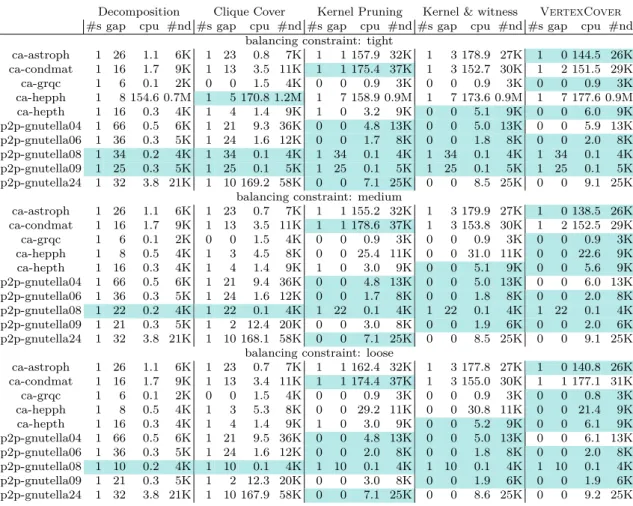
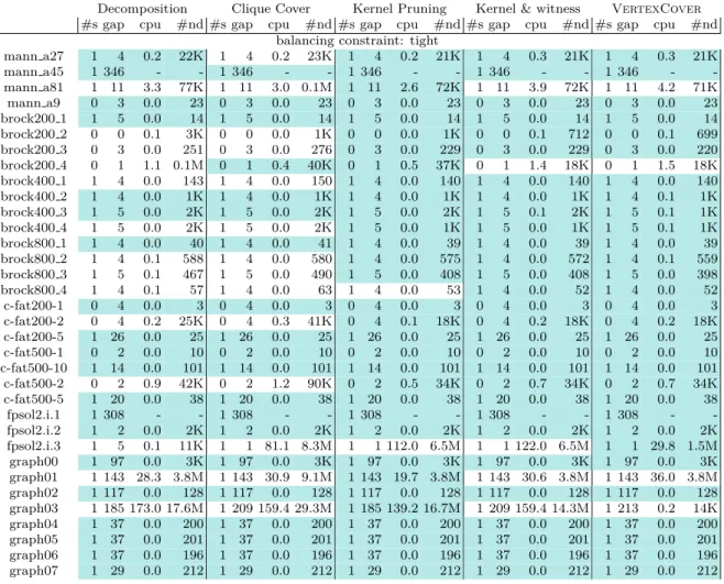
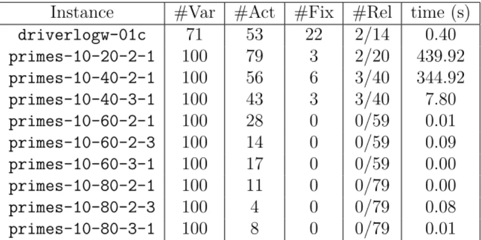
5.3 Experiments . . . 102
5.3.1 Implementation . . . 103
5.3.2 Methodology . . . 104
5.3.3 Results . . . 104
5.4 Conclusion and Future Research . . . 108
109 113 115 119 6 Conclusion Appendices A Omitted Proofs B Compendium of Problems
C Detailed Results for dimacs Instances
Chapter 1
Introduction
A considerable part of the current research in theoretical computer science finds its roots in Cobham’s thesis that problems solvable in practice are those with polynomial-time algorithms [40]. This has certainly proved to be a powerful in-sight: polynomial-time problems are usually easier to solve than NP-hard ones, and the study of complexity classes closed under polynomial-time reductions has raised deep questions about the structure of combinatorial problems. When the limitations of Cobham’s thesis are discussed, the same argument is often heard: there are impractical polynomial-time algorithms. Recently, the spectacular per-formance improvement of SAT solvers, which sometimes handle instances with millions of variables and prove nontrivial theorems on their own [87], suggests that there may exist reasonably practical exponential-time algorithms as well.
Ironically, the scientific community that studies the Constraint Satisfaction Problem (CSP) can be partitioned into two groups that are in perfect contradic-tion with Cobham’s thesis. The design of exponential-time algorithms is left into the hands of researchers whose main goal is practical solving, while in the mean-time complexity theorists have built an impressive catalog of subproblems with sophisticated polynomial-time algorithms and zero applications.
The present work is an attempt to bring this literature on tractable subprob-lems closer to being useful. The apparent lack of ambition of this statement is better understood with a measure of the obstacles that must be overcome. First, many of these tractable classes are defined by elusive algebraic properties and more often than not the complexity of testing for them is unknown. Second, hoping that practical CSP instances would fall readily into these highly structured classes on a regular basis is probably unrealistic, so mechanisms must be designed in order to make the framework more adaptable. Third, some of those polynomial-time algo-rithms were not designed with performance in mind and have critical flaws, such as an exponential dependency on the domain size. Fourth and last, the definition of CSP used in most theoretical works does not leave room for one of the most
widely used feature of constraint solvers, global constraints.
There has been remarkably little research on these issues, but we find they are fertile grounds for both theoretical and practical investigation. In this thesis we tend to stay on the theoretical side, but draw our motivation from practical considerations and even perform preliminary experiments to illustrate our results.
Outline of the Thesis
The necessary technical background is given in Chapter 2. The next three chapters present our contributions:
Chapter 3 addresses the issue of CSP instances that do not quite fit in any
well-studied tractable class. We investigate the possibility of computing efficiently a decomposition of a given instance into a reasonable number of subproblems that belong to a fixed “target” tractable class using the framework of strong
back-doors [135]. We observe that computing optimal decompositions is almost always
NP-hard, but a refined analysis through parameterized complexity shows that for certain tractable classes good decompositions can be found efficiently if they exist. We also introduce partition backdoors, which are generally easier to compute but may provide suboptimal decompositions. The content of this chapter has been published in [11] and [33], although this manuscript contains slightly different def-initions and a minor additional result.
Chapter 4 presents novel and highly non-trivial polynomial-time algorithms
for testing membership in tractable classes that have the property of being
con-servative. These classes have the double advantage of being very well understood
and working nicely with the partition backdoor approach developed in Chapter 3. Our main result is a proof that the conservative tractability criterion defined by Bulatov [21] is polynomially decidable. This is without a doubt the most signifi-cant contribution of this thesis, as it both answers a difficult theoretical question and sows the seeds for a potential efficient algorithm in the future (our algorithm being at the same time polynomial-time and extremely inefficient). We get as a byproduct of our methods an improved (“uniform”) algorithm for one of the most important conservative tractable classes, CSP over languages admitting conserva-tive edge polymorphisms. This chapter has been published in [31] and [30].
Chapter 5 approaches the subject of harnessing tractability in CSP from a
very different angle. It is commonplace for CSP solvers to allow modelling with predicates: for instance, the user can state “at most k distinct values can be used to assign these n variables”. Some predicates encapsulate NP-hard problems, and
making meaningful deductions from these constraints is very difficult for the solver. This time, we explore the possibility of using the (parameterized) tractability results for the encapsulated problems in order to speed up the resolution of CSP instances. For this, we define formally loss-less kernelization, a new variant of kernelization dedicated to the context of constraint reasoning. We use the Vertex Cover problem as a case study to showcase our ideas. The experimental part of this chapter has been published in [34].
Chapter 2
Background
This chapter introduces the fundamentals of constraint satisfaction and parame-terized complexity, which form the technical core of the present thesis. We will on purpose present more material than is absolutely necessary in order to help the reader understand the broader scientific context. This background will be comple-mented by small sections spread between our contributions which will introduce auxiliary concepts, notation and results as they are needed. We will only assume from the reader familiarity with elementary notions of mathematics and compu-tational complexity.
This chapter is organized as follows:
• Section 2.1 defines the Constraint Satisfaction Problem and introduces basic notation.
• Section 2.2 is a survey of tractable classes for CSP based on restrictions of the constraint language. This section is given special emphasis because its content will serve as a basis for our own contributions presented in Chapters 3 and 4.
• Section 2.3 complements this survey by a quick overview of known tractable classes obtained by imposing restrictions on the constraint (hyper)graph. Knowledge of these tractable classes is not required to understand our results or their significance, but we feel that omitting them would give the reader an excessively truncated view of tractability in CSP.
• Finally, Section 2.4 introduces parameterized complexity, which will be an integral part of our arsenal in our attempt to harness the tractable classes presented in Section 2.2.
We note that tractability results that do not fall within the scopes of Sec-tions 2.2 and 2.3 exist. These tractable classes are called hybrid. However, they are quite scattered and tend to be relatively small in general. For detailed informa-tion on these classes, we direct the reader to the recent surveys on the complexity of CSP [43][32].
2.1
Constraint Satisfaction Problems
The Constraint Satisfaction Problem (CSP) is a common formalism for combi-natorial problems that can be expressed as deciding if there exists an assignment to a set of finite-domain variables that satisfies a set of constraints. For example, solving a system of equations over a finite field is a problem of this kind; in this case the constraints are equations that must hold. In 3-SAT, the variables are Boolean and constraints are ternary clauses that must be satisfied. CSP gener-alizes both by only assuming that constraints are relations imposed on subsets of variables. The first explicit mention of this problem is found in a 1974 paper by Montanari [114].
Definition 1. A CSP instance is a triple (X , D, C), where
• X is a finite set of variables; • D is a finite set of values;
• C is a finite set of constraints, that is, pairs (SC, RC) where SC is a tuple of variables (the scope of C) and RC ⊆ D|SC| is a relation over D.
A solution to a CSP instance is an assignment φ : X → D such that ∀(SC, RC) ∈ C, φ(SC) ∈ RC (where φ is the operation on tuples of variables obtained by com-ponentwise application of φ). The problem is to decide if a solution exists, which is NP-complete [98]. In this definition, variables do not come with individual domains: variable-specific domain restrictions must be enforced using unary con-straints. Unless explicitly stated otherwise, we will assume that all relations are given in input as tables of tuples.
Remark 1. This last assumption has very important implications. For instance,
it implies that SAT (with unbounded clause arity) is not a subproblem of CSP. More generally, in many areas of mathematics equations are never represented as explicit lists of solutions. Doing so may change the complexity drastically by inflating exponentially the input size. However, for other problems in which the arity of the relations is naturally bounded, such as Graph k-Coloring, this hypothesis is harmless. In the more practice-oriented literature, it is common to
represent a relation R as the set of tuples that is accepted by a certain polynomial-time algorithm δR. This gives more latitude to CSP solvers for handling internally high-arity constraints, and makes the modelling phase noticeably easier by allowing the use of predicates. Families of relations represented intentionally are usually called global constraints. However, with this framework for relations the problem becomes much less interesting from a complexity-theoretic point of view since every NP problem becomes technically a CSP with a single constraint. These two definitions of CSP coexist peacefully in the literature because the constraint programming community is strongly polarized; the choice of encoding for relations is usually clear from the research topic. Unfortunately, the scope of this thesis is quite wide and will cover both settings. We will try to reduce ambiguity as much as possible.
Example 1. The input of the Betweenness problem is a set U of n elements
and a set T of ordered triples of distinct elements of U . The question is: is it possible to find a total ordering >U of U such that for each triple (a, b, c) ∈ T , either a >U b >U c or c >U b >U a? Betweenness is NP-complete [119], and can be easily encoded in CSP as follows. The domain is {1, . . . , n} and we have one variable xu for each u ∈ U . Between any two distinct variables xu, xv we add the constraint xu 6= xv. This ensures that solutions will always be bijections between U and {1, . . . , n}. Then, for each triple (a, b, c) ∈ T we add on (xa, xb, xc) a constraint with predicate R(xa, xb, xc) ⇐⇒ (xa > xb > xc) ∨ (xc > xb > xa), where > is the usual ordering on N. Note that these constraints have O(n3) tuples, so the resulting instance has polynomial size. It is easy to see that an assignment
φ is a solution to the CSP instance if and only if the ordering >U such that
a >U b ⇐⇒ φ(xa) > φ(xb) is a solution to the instance of Betweenness.
Equivalent formulations. CSP is known under multiple names. In logic, CSP
corresponds to special types of first-order formulas that allow only existential quan-tification and conjunctions of relational predicates. These formulas are called
primitive positive. In database theory, CSP instances correspond to conjunctive queries. CSP can also be formalized as a homomorphism problem as follows. A signature is a finite set σ of relation symbols Ri, each with a specified arity ki. A
relational structure A over σ, or σ-structure, is a finite universe A together with
one relation RA
i ⊆ Aki for each symbol Ri ∈ σ. If I = (X , D, C) is a CSP in-stance and σI = {R1, . . . , Rm} is the set of all relation symbols that appear in its constraints, the left-hand side structure of I is the σI-structure AL with universe X and for each i, the tuples of RAL
i are the scopes of constraints whose relation is Ri. The right-hand side structure of I is the σI-structure AR with universe D and for each i, RAR
i is the relation Ri. The solutions to I are then exactly the mappings φ : X → D such that φ(RAL
i ) ⊆ RA R
the homomorphisms from AL to AR.
CSP solving. CSP is a popular choice for encoding real-world problems in artificial intelligence and operational research. The reason is twofold: modelling is intuitive (much more so than Integer Linear Programming or SAT), and CSP solvers perform quite well in practice despite the obvious exponential worst-case. For readers completely unfamiliar with practical CSP solving, let us recall the basic skeleton of most CSP solvers.
Backtracking search. The search space is the set of all possible assignments
to the variables. The typical solver will explore depth-first a search tree, picking a variable-value pair (x, d) at each node and branching on the two cases x ← v and x 6= v. When the algorithm detects that the succession of decisions leading to a node makes the instance unsatisfiable, it reverses the last decision (it backtracks) and continues the exploration from there. The heuristic that chooses the value (x, v) to branch on is critical as even a single poor decision may have devastating consequences. The design of such heuristics is one of the motivations for our results in Chapter 3.
Propagation. At each node of the search tree, the solver uses a
polynomial-time algorithm to shrink the problem by identifying inconsistent assignments. Those rules are typically variants of local consistency methods (such as en-forcing generalized arc-consistency, described in Section 2.2.3, Remark 2). Propagation algorithms are delicate tradeoffs between pruning quality and time complexity; an overzealous algorithm might backfire by spending a con-siderable amount of time to prune assignments that would be much more easily ruled out after a few additional decisions. The main contribution of Chapter 5 is a novel theoretical framework for the conception of such algo-rithms.
In modern implementations these components are often complemented with
learn-ing [52][99], which infers new valid constraints by analyzlearn-ing past failures in the
search tree and has been hugely successful in SAT solvers [115]. Other features commonly sighted include (but are not limited to) symmetry-breaking [75], local search procedures [97] and alternative exploration strategies such as breadth-first search and limited discrepancy search [82].
Notation. In the subsequent chapters we will manipulate CSP instances in
many ways, and for this we need to introduce some elementary notations.
Tuples and scopes. Throughout the thesis, tuples will be delimited by
Given a tuple t and I ⊆ {1, . . . , |t|}, we denote by t[I] the projection of t onto I. We will give special treatment to constraint scopes and sometimes treat them as sets of variable occurrences rather than tuples. For instance, if SC is a scope and we pick x ∈ SC, the operation SC\x will remove x from
SC but not every occurrence of the variable pointed by x. If C = (SC, RC) is a constraint, t ∈ RC and x ∈ SC, we will use the shorthand t[x] for “t[i] with i such that S[i] = x”. This will greatly alleviate the notational burden by reducing the use of integer indexes.
Operations on CSP instances. Given a constraint C = (SC, RC) and a
subset of variables X1 ⊆ X , we denote by C[X1] the projection of C onto X1 (which is null if SC does not contain any variable in X1). The projection of a CSP instance I = (X , D, C) onto X1 ⊆ X is the instance I|X1 = (X1, D, C
∗) with C∗ = {C[X1] | C ∈ C}. A partial solution to I is a solution to some projection of I. Given a subset X1 ⊆ X and an assignment ψ : X1 → D, we denote by I[X1 ← ψ(X1)] the instance obtained from I by removing from each constraint relation the tuples t such that t[x] 6= ψ(x) for at least one
x ∈ X1, and then projecting I onto X \X1. We will say that I[X1 ← ψ(X1)] is the residual instance after application of the partial assignment ψ to X1.
Constraint languages. We will use R(.) and S(.) as operators that return
respectively the relation and the scope of a constraint. A constraint language over a set D is a set of relations over D, and the language L(I) of a CSP instance I = (X , D, C) is the set {R(C) | C ∈ C}. We will use D(Γ) to denote the domain of a constraint languages Γ, that is, the set of all values that appear in at least one tuple. Because constraint languages are sets of relations and relations are sets of tuples, we will use square brackets as delimiters for relations to avoid confusion.
2.2
Language-based Tractable Classes
A natural way to study the fine-grained complexity of CSP is to impose a fixed catalog of relations that are available for modelling instances and see how that affects the complexity. This type of restriction is often referred to as non-uniform
CSP, and the rich theory that has been built around it will be the background for
many of our own contributions.
Definition 2. Let Γ be a constraint language. We denote by CSP(Γ) the
restric-tion of CSP to instances I such that L(I) ⊆ Γ.
Well-known problems which are naturally of this form are legion. For instance, Graph k-Coloring is exactly CSP({6=k}) where 6=k is the disequality over a
k-element domain, and k-XORSAT is CSP(Γ⊕) where Γ⊕ contains all XOR-clauses of arity at most k. Because of the sheer diversity of possible constraint languages Γ, one could expect a rich complexity landscape where, depending on Γ, CSP(Γ) can be in P, NP-complete, or in one of the infinitely many intermediate complexity classes whose existence is proven by Ladner’s Theorem [106] assuming P 6= NP. The starting point for much of the current research is the observation that non-uniform CSP is, from a logic point of view, the largest subclass of NP that might contain only P and NP-complete problems [62]; in the same paper Feder and Vardi conjectured that it is the case, at least for finite languages.
Conjecture 1 (The Dichotomy Conjecture [62]). For every finite constraint lan-guage Γ, CSP(Γ) is either polynomial-time or NP-complete.
More that twenty years have passed and this conjecture is still open. Much of the initial research on non-uniform CSP consisted in disparate tractability or hardness results, with no unified framework to relate these results to each other [128][133][95]. This issue was solved by the algebraic approach to non-uniform CSP, formally introduced in a seminal 1997 paper by Cohen, Gyssens and Jeavons [94] but already suggested in Feder and Vardi’s original work [62]. This approach has been the foundation of most of the recent successes [21][19][8]. The central idea is to relate the complexity of non-uniform CSP to the identities satisfied by certain closure operations called polymorphisms.
2.2.1
Expressive Power of Constraint Languages
Let Γ be a fixed, finite constraint language. The textbook approach to prove that CSP(Γ) is NP-complete is to pick another language Γ∗ known to be NP-complete and patiently build gadgets for each R ∈ Γ∗ using only relations from Γ. The strategy of the algebraic approach to CSP is to study the complexity of constraint languages not by looking directly at the relations, but at the gadgets that can or cannot be made from them.
What we call gadget is generally a CSP instance whose solution set, when projected onto a specific subset of variables, is the desired relation. This notion of “CSP plus projections” is captured by formulas called pp-definitions.
Definition 3. A relation R has a pp-definition in a constraint language Γ if it
can be defined via a formula using only relations from Γ, conjunction, existential quantification and the equality relation.
We also say that R is expressible over Γ. By extension, a language has a pp-definition in Γ if and only if each of its relations has one.
Definition 4. Let Γ be a constraint language. The relational clone of Γ, denoted
by hΓi, is the set of all relations pp-definable in Γ.
If Γ∗ ⊆ hΓi, then CSP(Γ∗) is (logspace) reducible to CSP(Γ) because we can turn every relation in Γ∗ into a gadget over Γ [94]. This improvement alone already simplifies greatly the task of classifying the complexity of all constraint languages, because it implies that we need not distinguish two languages that generate the same relational clone. The next step is to find a way to characterize nicely which relations are found in hΓi.
2.2.2
Polymorphisms
Polymorphisms are componentwise closure operations that can have the powerful property of witnessing that a given relation R does not belong to hΓi.
Definition 5. Let Γ be a constraint language over a domain D and k > 0 be a
natural number. An operation f : Dk → D is a polymorphism of Γ if and only if
∀R ∈ Γ, ∀t1, . . . , tk ∈ R, f (t1, . . . , tk) ∈ R
where f is the operation on tuples obtained by componentwise application of f . The set of polymorphisms of a given constraint language contains every projec-tion over its domain and is closed under composiprojec-tion. It is therefore a (concrete)
clone. The link with relational clones is made explicit in the next proposition by
Geiger, which dates back to 1968.
Proposition 1 ([74]). If Γ and Γ∗ are constraint languages over the same domain
D, then Γ∗ ⊆ hΓi if and only if every polymorphism of Γ is a polymorphism of Γ∗. This means in particular that in order to show that a constraint language Γ∗ is
not expressible over Γ, we need only produce a single polymorphism of Γ that does
not preserve Γ∗. Unfortunately, in the worst case the size of this polymorphism can be exponentially large and deciding expressibility is co-NEXPTIME-hard in general [134][132].
Intuitively, the computational hardness of a language Γ can only increase as hΓi gets bigger. Thus, if Γ has very nontrivial polymorphisms (i.e. operations that are polymorphisms of few relations) then hΓi will be severely restricted and Γ has a chance to be tractable. This relationship between relational clones and clones of polymorphisms is quite tight as a Galois connection can be established between the two [92].
Example 2. Let us consider the language Γ3-LINpof all 3-variables linear equations over GF(p) for a given prime natural number p ≥ 2. CSP(Γ3-LINp) is easily seen as polynomial-time via Gaussian elimination, and thus it must admit nontrivial polymorphisms. Let R(x, y, z) ⇐⇒ ax + by + cz = d be an equation over GF(p), and let f be such that f (d1, d2, d3) = d1− d2+ d3. Observe that if (t1, t2, t3) =
((x1, y1, z1), (x2, y2, z2), (x3, y3, z3)) are tuples of R then
a f (x1, x2, x3) + b f (y1,y2, y3) + c f (z1, z2, z3)
= a (x1− x2+ x3) + b (y1− y2 + y3) + c (z1− z2+ z3) = d
and hence f (t1, t2, t3) ∈ R. This means that f is a polymorphism of Γ3-LINp; this type of group-theoretic polymorphism is highly nontrivial and is a particular case of Mal’tsev polymorphisms, which will be discussed in Section 2.2.4.
Now, we can start asking the important question: what makes a polymorphism desirable? We aim to identify polymorphisms that imply the tractability of any language they preserve, so they must enforce a strong structural property to the relational clone or, equivalently, to the clone of polymorphisms. The study of such properties is the main topic of universal algebra, and they are usually presented in the form of identities satisfied by the operations (here, polymorphisms), where identities are universally quantified equations over operation symbols and domain variables.
Throughout the thesis we will make use of a number of different properties for polymorphisms, and many of them will appear in multiple sections or chapters. For simplicity, we have gathered them in the next definition. The wavy equality sign ≈ signifies that the variables (x, y, z, etc.) are universally quantified over the domain.
Definition 6. Let f be an operation of arity k. We say that f is
• idempotent if
f (x, . . . , x) ≈ x
• conservative if ∀(x1, . . . , xk),
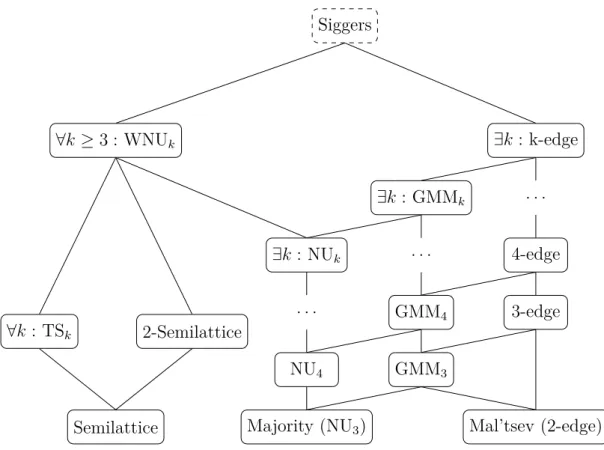
f (x1, . . . , xk) ∈ {x1, . . . , xk} • a Siggers operation if k = 4 and
• a weak near-unanimity (WNU) operation if k ≥ 3 and
f (y, x, x, . . . , x, x) ≈ f (x, y, x, . . . , x, x) ≈ . . . ≈ f (x, x, x, . . . , x, y)
• a near-unanimity (NU) operation if k ≥ 3 and
f (y, x, x, . . . , x, x) ≈ f (x, y, x, . . . , x, x) ≈ . . . ≈ f (x, x, x, . . . , x, y) ≈ x
• a majority operation if k = 3 and
f (x, x, y) ≈ f (x, y, x) ≈ f (y, x, x) ≈ x
• a minority operation if k = 3 and
f (x, x, y) ≈ f (x, y, x) ≈ f (y, x, x) ≈ y
• a Mal’tsev operation if k = 3 and
f (x, x, y) ≈ f (y, x, x) ≈ y
• a generalized majority-minority (GMM) operation if k ≥ 3, and ∀(a, b) either
∀(x, y) ∈ {a, b}, f (y, x, . . . , x) = f (x, y, . . . , x) = . . . = f (x, x, . . . , y) = x or
∀(x, y) ∈ {a, b}, f (y, x, . . . , x) = f (x, x, . . . , y) = y • a (k-1)-edge operation if k ≥ 3 and
f (x, x, y, y, y, . . . , y, y) ≈ y f (x, y, x, y, y, . . . , y, y) ≈ y f (x, y, y, x, y, . . . , y, y) ≈ y f (x, y, y, y, x, . . . , y, y) ≈ y . . . f (x, y, y, y, y, . . . , x, y) ≈ y f (x, y, y, y, y, . . . , y, x) ≈ y
• a totally symmetric (TS) operation (or set operation) if ∀(x1, . . . , xk, y1, . . . , yk), {x1, . . . , xk} = {y1, . . . , yk} ⇒ f (x1, . . . , xk) = f (y1, . . . , yk)
• a semilattice operation if k = 2 and
f (x, x) ≈ x, f (x, y) ≈ f (y, x), f (x, f (y, z)) ≈ f (f (x, y), z)
• a 2-semilattice operation if k = 2 and
f (x, x) ≈ x, f (x, y) ≈ f (y, x), f (x, f (x, y)) ≈ f (x, y)
These identities will allow us to present concise definitions of the most im-portant tractable classes of languages found in the literature. Polymorphisms have proved to be very valuable in capturing the deep computational properties of constraint languages; in particular they have been used to make a more specific version of Conjecture 1 that suggests a characterization of all tractable constraint languages.
Conjecture 2 ([26]). Let Γ be a constraint language. Γ is tractable if and only if it has a Siggers polymorphism.
This conjecture is the algebraic equivalent of the statement “a language is tractable if and only if it cannot simulate Positive 1-in-3-SAT”, where the “simulation” is done using a slightly improved version of pp-definability called
pp-interpretability. It can be made even more specific by assuming without loss
of generality that Γ is a digraph [62] and a core [26], that is, a language whose unary polymorphisms (endomorphisms) are all surjective. The conjecture has been confirmed in the case of 2- and 3-element domains [128][19], languages that contain all possible unary relations over their domain (which are called conservative and will be the main focus of Chapter 4) [21], and digraphs with no sinks and no sources [8] (generalizing the Hell-Neˇsetˇril theorem for undirected graphs [85]).
Now that we know what polymorphisms are and why they are important, we can finally survey the major tractability results for non-uniform CSP. We will partition them into two groups, one for each of the two main algorithmic techniques.
2.2.3
Tractability via Local Consistency
Local consistency techniques are the most common incomplete polynomial-time algorithms for CSP in practical works. The idea is as follows: instead of looking at the instance as a whole, focus on subproblems with a bounded number of variables and infer as much information as you can from them. This information will be embodied by new constraints, which may in turn be used to refine the reasoning made earlier on adjacent subproblems, and so on. This fundamental process is generally referred to as constraint propagation. If a contradiction is derived on a
subproblem then the instance has no solution. For certain constraint languages, the converse is true.
The ideas behind local consistency fit quite well the reasoning most humans would do when solving a CSP. Let us illustrate this with sudoku solving. What everybody does first is to create a list of potential values for each cell, and then review the constraints involving that cell (line, column and subtable) to see which values can be pruned. Whenever a list has been reduced, we check if the change can be used to prune additional values elsewhere, and so on. This is one of the simplest form of local consistency, where we derive new constraints (lists) on size-1 subproblems (cells).
Definition 7. Let k, l be fixed natural numbers such that 1 ≤ k ≤ l. A CSP
instance is (k, l)-minimal if
• Every subset of l variables is contained in the scope of a constraint, and • For every subset X of k variables, the projections onto X of any two
con-straints whose scopes contain X are identical.
For every fixed k, l a CSP instance I can be turned into an equivalent instance
I0 that is (k, l)-minimal in polynomial time. The algorithm adds new “allow-all” constraints on every size-l subset of variables, and then removes tuples from the constraints until all projections on k variables agree. Given a language Γ, we say that (k, l)-minimality decides CSP(Γ) if the above algorithm always derives a contradiction on unsatisfiable instances of CSP(Γ). In this case, we say that Γ has
width (k, l). We will use width k as a shorthand for width (k, k), k-minimality for
(k, k)-minimality and say that Γ has bounded width if it has width (k, l) for some
k, l.
For SAT, unit propagation is equivalent to enforcing 1-minimality, so Horn clauses are a simple example of width 1 language [128]. The idea was later gener-alized to show that all constraint languages with a semilattice polymorphism have width 1 [94]. A full characterization of width 1 languages can be found in Feder and Vardi’s work [62], which has been subsequently reformulated in algebraic terms by Dalmau and Pearson [49].
Theorem 1 ([49]). A constraint language Γ has width 1 if and only if it has totally symmetric polymorphisms of all arities.
An equivalent formulation requires a single totally symmetric polymorphism of arity D(Γ) [49].
Remark 2. A CSP instance is generalized arc consistent (GAC) if there is one
unary constraint D(x) on each variable x ∈ X , and for every d ∈ D(x) and
t[x] = d [111][112]. The tuple t is called a support for the pair (x, d). 1-minimal
instances are GAC, and if I is GAC then removing from every constraint every tuple that is not a support yields a 1-minimal instance, so GAC and 1-minimality are almost the same property. However, enforcing GAC does not involve remov-ing tuples from constraints of arity greater than 1 and as such this operation is much easier to perform on instances involving intentionally-represented relations; all that is needed is an algorithm δR+ for each relation R that computes in polyno-mial time the variable-value pairs that have supports in R. This algorithm δR+ is called a propagator, and the design of such algorithms for frequently used global constraints is a very active research topic [123][113][14]. Propagators will be the main motivation for the contributions presented in Chapter 5.
The set of all bijunctive clauses, defined as conjunctions of binary clauses, is an example of language that has width (2, 3) but not width 1 [128]. On the CSP front, connected row-convex constraints have been shown to have width 3 [55]. In both cases, the languages have actually a stronger property than bounded width called bounded strict width in which every consistent assignment to k variables (for some finite k) can be extended greedily to a solution of the whole instance. The polymorphisms characterizing bounded strict width were already identified by Feder and Vardi (although the terminology used was different) [62], and Jeavons, Cohen and Cooper gave a refined characterization [93]. We say that a relation is k-decomposable if it is equivalent to the conjunction of its projections on k variables.
Theorem 2 ([93]). Let Γ be a constraint language and k ≥ 3. The following statements are equivalent:
• Γ has strict width k;
• Γ has a near-unanimity polymorphism of arity k; • Every R ∈ hΓi is (k − 1)-decomposable.
While all width 1 and bounded strict width languages were identified at the early times of the algebraic era, progress on other languages on the bounded width hierarchy has been quite slow (aside from Bulatov’s proof that languages with a 2-semilattice polymorphism have width 3 [18]). In Feder and Vardi’s original work, a conjecture was formulated: every core constraint language Γ has either bounded width or the ability to count, which is informally the ability to simulate linear equations over a finite field [62]. More than fifteen years later, this conjecture was confirmed by Barto and Kozik [7] and a simple polymorphism-based characteriza-tion was given in [101].
Theorem 3 ([7][101]). A constraint language Γ has bounded width if and only if it has two weak near-unanimity polymorphisms f, g of respective arities 3, 4 satisfying
f (x, x, y) ≈ g(x, x, x, y)
Note that [7] only establish this result for core constraint languages, but it can easily be extended to the general case (see e.g. Lemma 6.4 of [36]). This condition is equivalent to having weak near-unanimity polymorphisms of all arities greater than 3. The tractable class of all languages of bounded width is very general, but at first sight it could suffer from a scalability problem: enforcing (k, l)-minimality is exponential-time in l, which can potentially be arbitrarily large depending on Γ. A surprising result, obtained independently by Bulatov and Barto, shows that every language of bounded width has width (2, 3) [6][20][23]. Combining this result with [47] we can draw the following picture.
Theorem 4 ([6][47]). Let Γ be a constraint language. Exactly one of the following statements is true:
• Γ has width 1;
• Γ has width (2, 3), but not width 2 nor width (1, l) for any l ≥ 1; • Γ does not have bounded width.
As it is, the class of languages of bounded width seems reasonably practical since enforcing (2, 3)-minimality is cubic time. In a very recent development, it was shown that enforcing singleton linear arc consistency (SLAC), a consistency notion weaker than (2, 3)-minimality, is an alternative decision procedure for languages of bounded width [100]. Enforcing SLAC is quadratic time. This series of highly nontrivial results is an edifying example of the impressive progress made in the understanding of tractable classes during the past decades.
2.2.4
Tractability via Few Subpowers
We have seen in the last section that the only obstruction to solvability by local consistency methods is the ability to simulate linear equations over a prime field. This leads us directly to the second major algorithmic technique, which can handle those equations as it generalizes Gaussian elimination. This type of algorithm differs fundamentally from local consistency methods as it uses polynomial-sized representations of all solutions to reason directly on the whole set of variables. For instance, the solution set of a system of homogeneous linear equations is a vector space, which can be represented very efficiently by a basis and the table of the field operations. In the few subpowers algorithm, the encoding of relations is very
similar: a small subset of tuples is kept (a generating set), and polymorphisms are used to combine them.
Initially, this generating set approach was borrowed from group theory [62] but since then it has been extended to more general algebras. The first major breakthrough of the approach was Bulatov’s proof that the existence of a Mal’tsev polymorphism implies tractability.
Theorem 5 ([17]). Every constraint language that admits a Mal’tsev polymor-phism is tractable.
The original proof was very involved, but it has been greatly simplified over the years [24][60]. The most recent algorithm encodes relations (i.e. solution sets) using frames, which are generating sets whose size is linear in both the domain size and the relation arity, and whose closure under the Mal’tsev polymorphism is the original relation [60]. The algorithm for solving CSP instances assuming a Mal’tsev polymorphism starts from a frame of the solution set of an instance with no constraints (i.e. Dn) and then adds the constraints one by one, updating the frame at each step. The final frame is empty if and only if the instance does not have a solution.
The first notable generalization of Bulatov’s result was obtained by Dalmau.
Theorem 6 ([46]). Every constraint language that admits a generalized majority-minority polymorphism is tractable.
Because near-unanimity polymorphisms are also generalized majority-minority polymorphisms, the languages they preserve can be solved by both local consis-tency and algorithms based on polynomial-sized representations.
The conclusion of this line of work was reached in [90] and [10] with a neces-sary and sufficient condition for this algorithmic technique to be applicable: the existence of an edge polymorphism.
Theorem 7 ([90]). Every constraint language that admits an edge polymorphism is tractable.
The algorithm for CSP over a language with an edge polymorphism is usually referred to as the few subpowers algorithm (hence the title of this section). If a language Γ does not have an edge polymorphism, the number of distinct relations of arity r in hΓi grows too fast with r for compact representations to exist [10], so this result determines precisely the reach of methods based on generating sets.
2.3
Structural Tractable Classes
In the relational structure homomorphism formulation of CSP seen in Section 2.1, non-uniform CSP corresponds to the case where the right-hand side structure is
fixed. A class of CSP is said to be structural if the left-hand side structure is restricted instead (but not fixed, because it would be trivially polynomial-time). None of our contributions will involve directly structural classes of CSP, but we feel that a quick overview would help the reader understand the big picture.
A hypergraph is a pair (V, E) where V is a finite set of vertices, and E is a collection of non-empty subsets of V called hyperedges. A graph is an hypergraph with only size-2 hyperedges, which are called edges.
Definition 8. The constraint hypergraph of a CSP instance (X , D, C) is the
hypergraph (X , {S(C) | C ∈ C}).
Definition 9. The primal graph of a CSP instance (X , D, C) is the graph (X , E)
such that (x, y) ∈ E if and only if there exists C ∈ C such that {x, y} ⊆ S(C). Like many other combinatorial problems, CSP is hard because of feedback effects. Restricting the primal graph to be acyclic turns arc-consistency into a complete decision procedure for CSP, and thus this fragment is tractable [53]. More generally, this property of having limited feedback can be extended using tree decompositions.
Definition 10. Let G = (V, E) be a graph. A tree decomposition of G is a
tree T = ({V1, . . . , Vn}, ET) whose vertices are subsets of V and such that (i) ∪i∈{1,...,n}Vi = V ;
(ii) ∀e ∈ E, there exists i such that e ⊆ Vi;
(iii) ∀v ∈ V , the sets Vi that contain v form a connected subtree of T .
The width of a tree decomposition is the size of the largest set Vi minus one, and the treewidth of a graph is the minimum width possible over all its tree de-compositions. The following theorem by Grohe shows the full strength of tree decompositions.
Theorem 8 ([79]). Let G be a recursively enumerable class of graphs. Assuming FPT 6= W[1]1, the restriction of CSP to instances whose primal graph is in G is
polynomial-time if and only if G has bounded treewidth.
The straightforward algorithm for solving a CSP instance assuming a tree de-composition works in a dynamic programming fashion, by computing full solution sets of the subinstances corresponding to the set Vi starting from the leaves. The bound on the size of each Vi ensures that the number of solutions is polynomial.
1A common complexity-theoretic assumption; additional information on these classes can be found in Section 2.4
An alternative is the k-consistency algorithm, which becomes a decision procedure when the primal graph has treewidth at most k [65].
When considering restrictions on the constraint hypergraphs, the complexity landscape becomes a bit more varied. If the restriction entails bounded arity, every tractable case falls in the scope of Theorem 8 [79]. However, it is clear that this cannot be the case in general. For example, if the restriction only imposes the existence of an hyperedge that covers every vertex, the treewidth of the primal graph is not bounded but the associated CSP is polynomial-time: this hyperedge translates into a giant constraint that covers the whole instance, and solutions can only be found among its tuples.
Fractional edge covers assign to each hyperedge a weight in such manner that
for each vertex v, the weights of the hyperedges that contain v sum up to 1. The
fractional edge cover number is the minimum total weight over all fractional edge
covers. Grohe and Marx [80] showed that if a restriction on constraint hypergraphs entails a bounded fractional edge cover, not only the associated CSP is tractable but every instance has polynomially many solutions. Recall that the dynamic programming approach on (hyper)tree decompositions works well because each bag of vertices has few solutions; if the two approaches are mixed by defining the size of each bag as its fractional edge cover number rather than its number of vertices, we obtain the tractable restriction of CSP instances whose constraint hypergraphs have bounded fractional hypertree width. This is the most general structural tractability result known to date, but there is no matching hardness result.
Theorem 9 ([80]). Let H be a class of hypergraphs with bounded fractional hyper-tree width. The restriction of CSP to instances whose constraint hypergraph is in
H is polynomial-time.
There is a certain asymmetry between the results we presented for left- and right-hand side restrictions: in this section, we considered constraint hypergraphs but systematically ignored the relation symbols that label each hyperedge. With these labels taken into account the picture is not much different, as Theorem 8 carries over if H is only required to have bounded treewidth modulo homomorphic equivalence [79].
2.4
Parameterized Complexity
It is reasonable to say that an algorithm is efficient if it scales well when the in-stances become more difficult. Classical complexity theory is a direct application of this statement, in which the input size is implicitly regarded as a universal mea-sure for the intrinsic hardness of a given instance. This is quite coarse-grained;
maybe the algorithm performs very well on some distributions of inputs and terri-bly on others. When this situation arises, one can only wonder: is there a better measure of hardness than the input size?
Parameterized complexity aims to answer that question by measuring the ef-ficiency of an algorithm as a multivariate function of both the input size and an auxiliary measure, the parameter. The parameter will typically attempt to measure some structural property of the instance; in graphs problems, it can for example measure how tree-like the input graph is. If the time complexity of an algorithm scales well when the parameter k is fixed but the input size increases, we can narrow down the source of hardness to the structural property measured by k. Just like classical complexity, this multivariate analysis of algorithms can then be used to study problems.
A problem is parameterized if each instance x is paired with a nonnegative integer k called the parameter.
Definition 11. The class XP consists of all parameterized problems that can be
solved in time O(f (k)|x|g(k)) for some computable functions f and g.
This class of problems is an immediate application of the discussion above: if the parameter k is fixed, the complexity of the algorithm witnessing membership in XP grows polynomially with the input size. These parameterized problems are called slice-wise polynomial. However, XP is not what parameterized complexity is famous for, since the vast majority of the literature is concerned with a more ambitious class of problems.
Definition 12. The class FPT consists of all parameterized problems that can
be solved in time O(f (k)|x|O(1)) for some computable function f .
The problems in FPT are said to be fixed-parameter tractable. FPT exhibits the same property as XP: if the parameter is fixed, an FPT algorithm becomes polynomial-time. The major difference is that k now only contributes to the con-stant factor, and no longer to the degree of the polynomial. This distinction yields a huge difference in scalability because even a polynomial of degree 10 is largely impractical.
Example 3. The Vertex Cover problem is a classical NP-complete problem
that will be discussed in depth in Chapter 5. Vertex Cover takes as input a graph G = (V, E) and an integer p, and asks if there exists S ⊆ V of at most p vertices that intersects every edge in E. We will use p as the parameter. Member-ship in XP is straightforward since we can simply enumerate all |V |p subsets of at most p vertices.
To see that Vertex Cover parameterized by p is in FPT as well, let us consider the following algorithm A which takes as input G and a subset L of
vertices. If L intersects every edge in E, the algorithm returns true. Then, if |L| ≥ p we return false and otherwise we pick an edge e = (u, v) that does not intersect with L and return A(G, L ∪ {u}) ∨ A(G, L ∪ {v}). Now, let us see what happens when we invoke A(G, ∅). If A(G, ∅) returns true, at least one recursion call to A has been made with an input L of size at most p that intersects every edge, so the instance of Vertex Cover is satisfiable. Conversely, if the instance has a solution S then invoking A with L ⊂ S as input will make two recursion calls with respectively L ∪ {u} and L ∪ {v} for some edge {u, v}. Because S must intersect {u, v}, at least one of these calls will be with a set L0 ⊆ S such that |L0| = |L| + 1 and we can repeat the same argument inductively. Eventually, a recursion call will be made with L = S and A will return true. Therefore, because ∅ ⊆ S, A(G, ∅) will always return true if the instance is satisfiable.
The recursion tree of A has a branching factor of 2, its depth cannot exceed p and the amount of work at each node is polynomial, so A(G, ∅) gives its answer in time O(2p|G|O(1)). This is a simple illustration of the bounded search tree technique which will be used in Chapter 3.
Beyond Vertex Cover a number of problems have been shown to be FPT for parameters much better than the input size. The classes FPT and XP are nested, with FPT known to be a strict subset of XP [59]. Between FPT and XP, Downey and Fellows proposed a full hierarchy of intermediate parameterized classes [57]:
FPT ⊆ W[1] ⊆ W[2] ⊆ . . . ⊆ XP
where for each t, W[t] is believed to be a strict subset of W[t+1]; for instance, we know that FPT 6= W[1] unless the Exponential Time Hypothesis fails [37]. This hierarchy is called the W-hierarchy, or weft hierarchy. Each of these classes is closed under fpt-reductions, which are the parameterized counterparts to polynomial-time many-one reductions and defined as follows.
Definition 13. Let P and Q be parameterized problems. An fpt-reduction of P
to Q is an operation φ that maps every instance (x, k) of P to an instance (x0, k0) of Q such that
• x is a yes-instance if and only if x0 is,
• φ can be computed in time O(f (k)|x|O(1)) for some computable function f , and
• k0 ≤ g(k) for some computable function g.
Fpt-reductions differ from polynomial-time many-one reductions in two ways: they are allowed to be exponential-time as long as they are FPT, but they must
preserve the parameter. The two types of reductions are in general incomparable. Fpt-reductions provide a well-defined completeness theory for these classes, and through this notion they give the ability to show that a problem is fixed-parameter
intractable unless there is a collapse somewhere in the W-hierarchy. For instance,
the k-Clique problem parameterized by k is W[1]-complete [58], and Dominat-ing Set parameterized with solution size is W[2]-complete [57].
Over the years, the considerable scientific attention directed towards parame-terized complexity has resulted in a wealth of algorithmic techniques tailored for FPT algorithm design. Notable examples include bounded search trees (as in Ex-ample 3), iterative compression [122], color coding [3], and LP-branching [91]; a detailed survey of these techniques (and more) can be found in [45]. In Chapter 5 we will be particularly concerned with another technique, kernelization.
Definition 14. Let P be a parameterized problem. A kernelization of P is an
operation K that maps every parameterized instance (x, k) of P to a new instance (x0, k0) of the same problem such that
• K can be computed in polynomial time,
• k0 ≤ g(k) for some computable function g, and • |x0| ≤ f (k) for some computable function f .
The instance (x0, k0) is the kernel of (x, k). Kernelization is in essence a polynomial-time preprocessing routine whose performance in reducing the problem size is guaranteed in terms of the parameter. The philosophy is identical to that of the class FPT, as it captures algorithms that work well when the parameter is small. The idea is simply applied to polynomial-time preprocessing rather than exponential-time exact algorithms. Most kernelization algorithms work using a list of small, easily applicable reduction rules - the main technical challenge is often to prove that when these rules are no longer applicable, the size of the instance is bounded by a function of the parameter. Kernelization has been the subject of extensive research, with very small kernels obtained for a variety of problems (e.g. at most 2k vertices for Vertex Cover [117], or k6 clauses for Almost-2-SAT [103]), and new tools have been developed to prove kernelization lower bounds [15][86].
If a kernelization exists for a given parameterized problem, an FPT algorithm exists as well because employing bruteforce on the kernel is FPT. An important fact about kernelization is that the converse is true as well: if a problem is FPT, then it can be kernelized. To see this, assume that you have an algorithm with running time O(f (k)|x|O(1)) that solves your problem. Then, if the instance has size at least f (k), this algorithm is actually polynomial-time and we can use it
to compute a constant-sized kernel, which only depends on the satisfiability of the instance. Otherwise, we can leave the instance untouched since |x| ≤ f (k). Therefore, a kernel of size f (k) can be derived from the FPT algorithm. However, because f (k) will typically be exponential in k, this kernel is very poor; the true challenge is to find kernels that are polynomial-sized and as small as possible.
Chapter 3
Backdoors into Tractable
Constraint Languages
In general, tractable classes that can be solved by an algorithm whose complexity is a reasonable polynomial tend to be quite small, in the sense that they contain only highly structured instances. Furthermore, even assuming that every con-straint language that is not currently known to be NP-hard is tractable (which is as hopeful as one can be), the probability that a language comprised of a single loop-free random relation is tractable tends to zero as either the domain size or the maximum arity tends to infinity [110]. This effect is even more pronounced for random languages because they are at least as hard as each of their relations. In practice, even though industrial CSP instances are all but random it is quite un-likely that they fit nicely into one of the few well-studied tractable classes presented in Chapter 2.
The viewpoint adopted in this chapter is that it is possible to make broader use of the theoretical work on tractable classes by defining a proper notion of
distance between a given instance and an efficiently solvable restriction of CSP. In
this setting, this notion of distance to a tractable class H must be algorithmically meaningful: the instances at distance k should be easier to solve than instances at distance k + 1 (at least in terms of worst-case complexity), and there must exist a reasonably fast algorithm for solving instances k-distant from H if k is small. In the context of CSP and SAT, a natural measure of distance that satisfies our requirements is the strong backdoor size. Informally, a strong backdoor into a tractable class H is a subset of variables whose complete instantiation always yields a residual instance in H. If an instance has a size-k strong backdoor B into a class H, then it can be decomposed into at most |D|k instances in H by branching exhaustively on the possible assignments to B. The computation of the set B itself can be done either by enumerating all k-subsets of variables or by a more sophisticated method. Strong backdoors were introduced in [135] with the
original goal of explaining the performance of CSP and SAT solvers, and have attracted significant attention in the following years [125][56][72].
When approaching strong backdoors, one must make a clear distinction be-tween the solving phase, where the backdoor is known, and the computation of the backdoor. If a nontrivial backdoor B is already known then regardless of its size it is a useful information for a constraint solver, which can invoke a dedicated algorithm whenever the backtracking search procedure has assigned every variable in B (we omit small additional technical requirements here; variables outside B may have been assigned as well and the instance may have been reduced by aux-iliary inference, such as consistency algorithms). In fact, if the backdoor size k is quite large this approach is likely to be more efficient in practice than a straight de-composition of the instance into |D|ksubproblems. For example, if a CSP instance has 150 variables a backdoor of size 40 provides an uncompetitive decomposition but can still allow a general backtracking algorithm to prune a large number of branches, even if the backdoor is not used to guide the branching heuristic. As a direct consequence, improving the worst-case complexity of the solving phase is important but not critical for the usefulness of the framework.
The computation of the backdoor itself is a whole different matter. As k grows, deciding if a size-k strong backdoor exists becomes increasingly difficult while the information it would provide becomes less and less computationally relevant. The critical point is the (approximate) value of k for which the backdoor approach no longer yield any performance gain overall. If the backdoor detection algorithm scales poorly with k, the threshold will be reached very quickly and the applicabil-ity of the whole framework will be severely restricted. Therefore, it makes sense to focus on the detection phase (instead of the solving phase) and more precisely on algorithms that scale very favorably with the backdoor size k. To that endeavor the use of parameterized complexity theory is natural and k is the parameter of choice.
In this chapter we shall attempt to identify which properties of the tractable class H affect the parameterized complexity of detecting strong backdoors into H for the parameters k and k + r (backdoor size plus maximum arity). In a complementary fashion we also describe partition backdoors, a relaxation of strong backdoors that is noticeably easier to detect but may also be much larger.
3.1
Strong Backdoors
In this section we shall define formally all necessary notions and give a comprehen-sive overview of existing results on strong backdoor theory. While strong backdoors were originally defined in terms of subsolvers (in this case the target property is to be solvable by a given algorithm), we opt for another definition that only requires
the subproblems to belong to a given set of instances. This is roughly equivalent since we can always define the target set of instances to be exactly those solvable by the subsolver, or design the subsolver so that it only accepts the designated instances.
Definition 15. Let I = (X , D, C) be a CSP instance and H be a fixed set of
CSP instances. A strong backdoor of I into H is a subset of variables B ⊆ X such that ∀ φ : B → D, I[B ← φ(B)] ∈ H.
For the associated detection problem, we can either make H part of the input or define a detection problem for every fixed H. The latter is more adapted to our ultimate purpose, which is to identify which properties of H can make strong backdoors into H easier to detect.
Strong H-Backdoor Detection
Input: A CSP instance I = (X , D, C), an integer k
Question: Does I have a strong backdoor into H of size at most k?
We note that strong backdoors could easily be strengthened with additional inference after the backdoor variables are assigned. Our definition requires that every subproblem must belong to H, even those that are trivially unsatisfiable. While we have no doubt that extra layers of inference (such as arc consistency) could have a dramatic effect on the backdoor size, the backdoor is also likely to become unrealistically hard to compute. For instance, in the context of SAT even the very straightforward feature of empty clause detection (which adds to H every instance that contains an empty clause) makes backdoor detection substantially more difficult [56]. We believe that finding a form of inference that improves sufficiently the backdoor size to counterbalance the increased computational cost of detection is quite challenging. In this thesis we will only focus on the standard definition of strong backdoor and leave these considerations for future work.
Example 4 (Root sets). Following [51], given a binary CSP instance I = (X , D, C)
and a constraint C = ((x, y), R) ∈ C we write x → y (resp. y → x) if there exists a function f : D → D such that (a, b) ∈ R ⇐⇒ b = f (a) (resp.
(a, b) ∈ R ⇐⇒ a = f (b)). If either x → y or y → x, C (and by extension
R) is said to be functional. Using the → relation, one can associate every binary
instance I with a directed graph GI that describes the functional dependencies of the variables. One of the key ideas of [51] is that evaluating every complete instantiation of a root set of GI (a subset of vertices B such that every vertex can be reached from B via a directed path) is sufficient to decide the satisfiability of
I. Because of the functional dependencies, a root set is always a strong backdoor
procedure. The converse is false, but finding a minimum-size root set in a binary CSP has the advantage of being polynomial-time [51].
Because of the complete freedom left in the definition of the class H, strong backdoor detection covers a wide variety of problems as particular cases. For instance, if H is the set of all CSP instances whose constraint graph has some fixed property P then detecting a minimum-size backdoor into H can be reformulated as finding in the constraint graph the largest induced subgraph with property P (or, equivalently, a minimum subset of vertices whose removal leaves a residual graph with property P), a classical problem which has been extensively studied for many choices of P [109][81][89][29]. Orthogonally, some forms of symmetry breaking can be formulated in terms of strong backdoor detection. Given a CSP instance I = (X , D, C) a variable x ∈ X is irrelevant [16] if for every solution
φ : X → D and v ∈ D, the assignment φ0 : X → D such that φ0(y) = v if y = x and φ0(y) = φ(y) otherwise is also a solution. The set of all irrelevant variables of a CSP instance is exactly the complement of the minimum-size strong backdoor into the union of CSP({Dk| k ∈ N}) with the set of all unsatisfiable instances. An even more far-fetched example of strong backdoor detection would consider CSP as deciding if the input instance has an empty strong backdoor to the set of all satisfiable CSP instances. It is clear from these examples that if we wish to keep backdoor detection from being too wild we must restrict H to tractable classes of instances whose associated strong backdoor detection problem can be handled by relatively homogeneous algorithmic methods.
For CSP it is natural to focus on classes H of instances that are either struc-tural (definable by restrictions on the constraint hypergraph) or language-based (definable by restrictions on the constraint language). This excludes degenerate classes while still allowing most types of backdoor that have a nonzero probability of being useful in practice.
If H is structural, the complexity of Strong H-Backdoor Detection pa-rameterized by k is a pure graph theoretic problem. In CSP, the most interesting case arises when H is the set of all CSP instances whose primal constraint graph has treewidth bounded by a constant c; assuming FPT 6= W[1] and a bound on the constraint arities every tractable structural restriction of CSP must have bounded treewidth [79]. In this case Strong H-Backdoor Detection is (non-uniform) FPT because the class twc+ kv of all graphs obtained by adding at most k vertices to a graph with treewidth at most c is minor-closed and hence can be recognized in cubic time [124]. From a theoretical perspective this result essentially settles the complexity of detecting strong backdoors into (relevant) structural restrictions of CSP. It leaves however the practical questions completely unanswered since nei-ther the FPT algorithm itself nor its exact complexity is known (only its existence is proven by [124]). The most notable exception is the case c = 1 (that is,
![Figure 5.1: A non-rigid crown decomposition. The vertices of a minimum-size vertex cover of G[W ∪ I] that does not contain W are circled.](https://thumb-eu.123doks.com/thumbv2/123doknet/3132426.89157/98.892.288.678.216.487/figure-decomposition-vertices-minimum-vertex-cover-contain-circled.webp)