On the role of bulk viscosity in compressible reactive shear layer developments

an author's

https://oatao.univ-toulouse.fr/22758

https://doi.org/10.1016/j.euromechflu.2019.02.005

Boukharfane, Radouan and Martínez Ferrer, Pedro José and Mura, Arnaud and Giovangigli, Vincent On the role of

bulk viscosity in compressible reactive shear layer developments. (2019) European Journal of Mechanics - B/Fluids,

77. 32-47. ISSN 0997-7546

On the role of bulk viscosity in compressible reactive shear layer

developments

Radouan Boukharfane

a,b

, Pedro José Martínez Ferrer

a,c

, Arnaud Mura

a,∗

,

Vincent Giovangigli

d

a_{PPRIME UPR 3346 CNRS, ENSMA, 86961, Futuroscope Chasseneuil Cedex, France}

b_{ISAE-Supaero, BP 54032, 31055 Toulouse Cedex 04, France}

c_{Barcelona Supercomputing Center, C/ Jordi Girona, 29, Barcelona, 08034, Spain}

d_{CMAP UMR 7641 CNRS, Ecole Polytechnique, 91128 Palaiseau Cedex, France}

Keywords:

Bulk viscosity Shear layer

Direct numerical simulation Molecular transport

a b s t r a c t

Despite 150 years of research after the reference work of Stokes, it should be acknowledged that some confusion still remains in the literature regarding the importance of bulk viscosity effects in flows of both academic and practical interests. On the one hand, it can be readily shown that the neglection of bulk viscosity (i.e.,κ = 0) is strictly exact for mono-atomic gases. The corresponding bulk viscosity effects are also unlikely to alter the flowfield dynamics provided that the ratio of the shear viscosityµ to the bulk viscosityκremains sufficiently large. On the other hand, for polyatomic gases, the scattered available experimental and numerical data show that it is certainly not zero and actually often far from negligible. Therefore, since the ratioκ/µcan display significant variations and may reach very large values (it can exceed thirty for dihydrogen), it remains unclear to what extent the neglection ofκholds. The purpose of the present study is thus to analyze the mechanisms through which bulk viscosity and associated processes may alter a canonical turbulent flow. In this context, we perform direct numerical simulations (DNS) of spatially-developing compressible non-reactive and reactive hydrogen–air shear layers interacting with an oblique shock wave. The corresponding flowfield is of special interest for various reactive high-speed flow applications, e.g., scramjets. The corresponding computations either neglect the influence of bulk viscosity (κ =0) or take it into consideration by evaluating its value using theEGlib library. The qualitative inspection of the results obtained for two-dimensional cases in either the presence or the absence of bulk viscosity effects shows that the local and instantaneous structure of the mixing layer may be deeply altered when taking bulk viscosity into account. This contrasts with some mean statistical quantities, e.g., the vorticity thickness growth rate, which do not exhibit any significant sensitivity to the bulk viscosity. Enstrophy, Reynolds stress components, and turbulent kinetic energy (TKE) budgets are then evaluated from three-dimensional reactive simulations. Slight modifications are put into evidence on the energy transfer and dissipation contributions. From the obtained results, one may expect that refined large-eddy simulations (LES) may be rather sensitive to the consideration of bulk viscosity, while Reynolds-averaged Navier–Stokes (RANS) simulations, which are based on statistical averages, are not.

1. Introduction

The bulk (or volume) viscosity

κ

, which can be related to the

second (or dilatational) viscosity coefficient

λ

, is associated to

the vibrational and rotational energy of the molecules. From the macroscopic viewpoint, it characterizes the resistance to dilatation of an infinitesimal bulk element at constant shape [1]. It is strictly zero only for dilute monoatomic gases and this theoretical result is often used to discard it, regardless of the nature or internal

∗

Corresponding author.

E-mail address:arnaud.mura@ensma.fr(A. Mura).

structure of the fluid as well as the flowfield conditions. However, acoustic absorption measurements performed at room tempera-ture have shown that the ratio of the volume to the shear viscosity

κ/µ

may be up to thirty for hydrogen at room temperature [2], and

recent analyses of reactive multicomponent high-speed flows have confirmed that it is not justified to neglect it, except for the sake of simplicity [3]. The dilatational viscosity is important in describing sound attenuation in gaseous media, and the absorption of sound energy into the fluid depends itself on the sound frequency, i.e., the rate of fluid expansion and compression. For polyatomic gases, the

available measurements of

κ

, which remains quite seldom due

to the complexity of its determination, show that it is certainly not zero and actually far from negligible. It is also noteworthy

https://doi.org/10.1016/j.euromechflu.2019.02.005 0997-7546/©2019 Elsevier Masson SAS. All rights reserved.

that theoretical analyses do show that

κ/η

is at least of the order

of unity. Therefore, since the ratio

κ/µ

can display significant

variations and may reach very large values, it is unclear to what

extent the Stokes hypothesis (i.e.,

λ = −

2

µ/

3 or

κ =

0) may be

used for compressible and turbulent flows of gases featuring a ratio

κ/µ

greater than unity.

In either an expansion or a contraction of the gas mixture, the work done by the pressure modifies immediately the translational energy of the molecules, while a certain time-lag is needed for the translational and internal energy to re-equilibrate through

inelastic collisions [4]. This can be described through a system of

two coupled partial differential equations written for the internal and translational temperatures, with a pressure-dilatation term that acts as a source term in the translational temperature budget. The volume (or bulk) viscosity is associated to this relaxation phe-nomenon and it is evaluated from this internal energy relaxation time-lag. The evaluation of this property for a mixture of poly-atomic gases is far from being an easy task since the kinetic theory of gases does not yield an explicit expression for this transport coefficient, but instead linear systems that must be solved [5]. The corresponding systems are derived from polynomial expansions of the species’ perturbed distribution functions. The bulk viscosity

is obtained here using the library

EGlib

developed by Ern and

Giovangigli [6,7]. It is evaluated as a linear combination of the pure species volume viscosities, which require the evaluation of various collision integrals [5].

The impact of bulk viscosity effects has been previously analyzed in several situations including shock-hydrogen bubble interactions [3], turbulent flames [8], compressible boundary

lay-ers [9], shock-boundary layer interaction [10], and planar

shock-wave [11]. All these studies confirm that the bulk viscosity

ef-fects may be significant. The purpose of the present work is to assess its influence in regard to both the instantaneous and sta-tistical features of canonical compressible turbulent multicompo-nent flows. Using direct numerical simulation (DNS), we

investi-gate the impact of the bulk viscosity coefficient

κ

on the spatial

development of reactive and non-reactive compressible mixing layers interacting with an oblique shock wave. Such a canonical flowfield is typical of the shock–mixing layer interactions that

take place in compressible flows of practical interest [12]. For

instance, supersonic jets at high nozzle-pressure ratio (NPR) give rise to complex cellular structures, where shocks and expansions

waves interact with the turbulent outer shear layer [13]. It is also

relevant to scramjet intakes and combustors, where shock waves interact with the shear layers issued from the injection systems. On the one hand, it is clear that the occurrence of shock waves in supersonic combustors induces pressure losses that cannot be avoided but, on the other hand, the resulting shock interactions with mixing layers contribute to scalar dissipation (i.e., mixing)

rates enhancement [14], and may favor combustion stabilization

in high-speed flows.

The present manuscript is organized as follows: the

mathemat-ical model is presented in the next section (i.e., Section2), which

also includes a short description of the numerical methods. The details of the computational setup are subsequently provided in

Section3. Section4 gathers all the results issued from (i)

two-dimensional numerical simulations of both inert (4.1) and reactive

(4.2) cases, and (ii) the three-dimensional case, which is analyzed

in4.3. Finally, some concluding remarks and perspectives for

fu-ture works are presented in Section5.

2. Mathematical description and computational model

In this work, the in-house massively parallel DNS solver

CREAMS

is used. It solves the unsteady, three-dimensional set of com-pressible Navier–Stokes equations for multicomponent reactive mixtures [15]:

∂

t

(ρ) + ∇ · (ρ

u

) =

0

,

(1a)

∂

t

(ρ

u

) + ∇ · (ρ

u

⊗

u

) = ∇ · σ,

(1b)

∂

t

(ρ

Et

) + ∇ · (ρ

uEt

) = ∇ · (σ ·

u

−

J

) ,

(1c)

∂

t

(ρ

Yα

) + ∇ · (ρ

uYα

) = −∇ · (ρ

VαYα

) + ρ ˙ω

α

,

(1d)

where t denotes the time,

∇

is the spatial derivative operator, u is

the flow velocity,

ρ

is the density,E_t

=

e+u

·

u

/

2 is the total specific energy (obtained as the sum of the internal specific energy, e, and

kinetic energy), Y_αis the mass fraction of chemical species

α

(with

α ∈

S

= {

1

, . . . ,

N_sp

}

), V_αis the diffusion velocity of species

α

,J

is the heat flux vector and

ω

˙

_αrepresents the chemical production

rate of species

α

. The integerNspdenotes the number of chemical

species.

The above set of conservation equations(1)requires to be

com-pleted by constitutive laws. In this respect, the ideal gas mixture

equation of state (EoS), P

=

ρ

RT

/

W withRthe universal gas

constant, is used to relate the pressure P to the temperature T .

In this expression, the quantityWdenotes the molar weight of

the multicomponent mixture, which is obtained as the sum of the

molecular mass of each individual speciesW−1

=

∑

Nsp

α=1Yα

/

Wα. Within the framework of the kinetic theory of dilute polyatomic

gas mixtures, the molecular diffusion velocity vector V_α,

α ∈

S,

heat flux vectorJ, and second-order stress tensor

σ

are expressed

as follows:

ρ

V_αY_α

= −

∑

β∈S

ρ

Y_αDα,β

(

d_β

+

χ

_βX_β

∇

(

ln T

) ) ,

(2a) J

=

∑

α∈S

ρ

V_αY_α

(

h_α

+

RT

χ

α W_α

)

−

λ

_T

∇T

,

(2b)

σ = −

PI

+

τ = −

PI

+

µ (∇

u

+

∇

u⊺

_{) + λ (∇ ·}

_u

₎

_I

_,

_(2c)

whereDα,βare the multicomponent diffusion coefficients, dα,

α ∈

S, the species diffusion driving forces,

χ

_α the rescaled thermal

diffusion ratios, X_αthe species mole fractions, h_αthe enthalpy per

unit mass of the

α

th species, and

λ

Tthe thermal conductivity. The

diffusion driving force d_αof the

α

th species is given by d_α

=

∇X

_α

+

(

X_α

−

Y_α

) ∇ (

ln P

)

. The quantity

µ

denotes the shear viscosity

and

λ

denotes the second (or dilatation) viscosity coefficient.

The bulk viscosity coefficient

κ

appears explicitly in the

expres-sion of the viscous stress tensor

τ

. A relationship between the bulk

viscosity

κ

and viscosity coefficients

µ

and

λ

can be deduced from

the expression of the total pressure, which can be evaluated as the component of the spherical tensor based on the trace of the total stress tensor

σ

:

−

tr(

σ

) 3

= −

i=3

∑

i=1

σ

ii 3

=

P

−

(

λ +

2 3

µ

)

∇ ·

u

=

P

−

κ∇ ·

u (3)

The second term in the right-hand-side of the above expression is

the dilational contribution, which defines the bulk viscosity as

κ =

λ+

2

µ/

3. As mentioned above, the Stokes’ hypothesis, stating that

λ = −

2

µ/

3 (and hence

κ =

0), is often retained as a simplifying assumption. Many efforts have been devoted to the derivation of relationships between the bulk viscosity and fundamental fluid

properties [16,17]. If we consider a single polyatomic gas with a

unique internal energy mode, the internal energy relaxation time

τ

int_{can be related to the bulk viscosity [4,18]:}

κ = (

PR

/

c_v2

) ·

cint

τ

int

,

(4)

when the relaxation time is smaller than fluid characteristic times.

In the above expression, cintdenotes the internal heat capacity and

c_vthe specific heat at constant volume. When there are several

the above simple expression is replaced by the solution to a linear

system [19]. Within the Monchick and Mason approximation [20],

neglecting complex collisions characterized by more than one

quantum jump, the reduced system is diagonal and yields

κ

[3]:

κ = (

PR

/

c_v2

) ·

∑

k∈P

Xkcintk

τ

int

k

,

(5)

where the integer P

=

1

, . . . ,

np_{is the polyatomic species}

index-ing set. The average relaxation time for internal energy of the kth species

τ

int

k is then expressed as:

c_kint

/τ

_kint

=

∑

l∈N

c_kl

/τ

_kl

,

(6)

where

τ

l

kdenotes the average relaxation time of internal energy

mode l for the kth species, and N is the internal energy mode indexing set.

The

CREAMS

solver is coupled with the

EGlib

library to esti-mate transport coefficients from the kinetic theory of gases [21]. In

this library, the optimized subroutines

EGSKm are used to evaluate

the bulk viscosity. The integer m

∈

_J2

,

6Kassociated to the subrou-tine name refers to retained level of approximation. The higher the value of m, the more expensive the algorithm but also the more accurate the bulk viscosity expression. Following the work of Billet et al. [3], the value m

=

3 is retained for the purpose of the present study. The shear viscosity and diffusion velocities are evaluated

with the routines

EGFE3

and

EGFYV

, respectively.

EGFLCT3

is used

to determine the thermal conductivity

λ

T and rescaled thermal

diffusion ratios

χ

_α. In this respect, some additional computations

showed that the extra time needed for m

=

4 and m

=

5 is

approximately 30% in comparison with the one needed for m

=

2

and m

=

3, while an additional time larger than 250% is required

for m

=

6 compared to m

=

2 and m

=

3.

The above system (1) is discretized on a Cartesian grid. A

seventh-order accurate WENO scheme is used to approximate inviscid fluxes, while an eighth-order accurate centered difference scheme is retained to approximate viscous and diffusive contribu-tions. Time integration is performed with a third-order accurate TVD Runge–Kutta scheme. The stiffness associated to the wide range of time scales involved in the description of the chemical

sys-tem is addressed using the Sundials

CVODE

solver [22]. A standard

splitting operator technique, similar to the one previously retained

in Ref. [23], is used. A detailed verification of the solver may be

found in Refs. [15,24].

3. Problem statement and computational setup

We study the interaction of an oblique shock with a spatially-developing shear layer. The upper stream corresponds to the fuel inlet, i.e., a mixture containing hydrogen, and the bottom inlet stream to vitiated air. Both two- and three-dimensional

com-putations are performed.Fig. 1provides a typical sketch of the

corresponding computational geometry and Table 1gathers the

values of the main parameters relevant to the present numerical simulation. The flow initialization is similar to the one retained in

Ref. [15]. Assuming equal free-stream specific heat capacity ratios,

the convective Mach number may be evaluated from Mc

=

(U1

−

U2)

/

(a1

+

a2), where a1and a2denotes the sonic speeds of streams 1 (oxidizer inlet stream) and 2 (fuel inlet stream) respectively. For

the present set of computations, it is equal to Mc

=

0

.

48. The

values of the velocity at the inlets are U1

=

1634

.

0 m

/

s at bottom (oxidizer stream) and U2

=

973

.

0 m

/

s at top (fuel stream).

The mixing layer flow is impinged by an oblique shock wave

that is issued from the oxidizer inlet stream (1) at the bottom

boundary. The oblique shock wave angle is

β =

33◦

, seeFig. 1. The geometrical parameters relevant to the present set of numerical

Table 1

Parameters of the shock–mixing layer interaction case.

Fuel Oxidizer Bottom

P (Pa) 94 232.25 94 232.25 129 951.0 T (K) 545.0 1475.0 1582.6 u1(m/s) 973.0 1634.0 1526.3 u2(m/s) 0.0 0.0 165.7 u3(m/s) 0.0 0.0 0.0 Mach (−) 1.6 2.12 1.93 YH2(−) 0.05 0.0 0.0 YO2(−) 0.0 0.278 0.278 YH2O(−) 0.0 0.17 0.17 YH(−) 0.0 5.60·10−7 5.60·10−7 YO(−) 0.0 1.55·10−4 1.55·10−4 YOH(−) 0.0 1.83·10−3 1.83·10−3 YHO2(−) 0.0 5.10×10 −6 _5.10×10−6 YH2O2(−) 0.0 2.50×10 −7 _2.50×10−7 YN2(−) 0.95 0.55 0.55 Table 2

Computational mesh description.

Lx1 Lx2 Lx3 Nx1 Nx2 Nx3 δω,0(m)

280 130 15 1640 750 180 1.44×10−4

simulations are provided inTable 2. The quantities Lx1, Lx2, and

Lx3 denote the computational domain lengths in each direction

normalized by the initial vorticity thickness

δ

_ω,0, while Nx1, Nx2,

and Nx3 are the corresponding numbers of grid points. In the

two-dimensional computations, only the x1- and x2-directions are

considered.

The flow is initialized with a hyperbolic tangent profile for the streamwise velocity component, while the other velocity compo-nents are set to zero. Species mass fractions and density are also set according to the following general expression:

ϕ

(x1

,

x2

,

x3)

=

ϕ

1

+

ϕ

2 2

+

ϕ

1

−

ϕ

2 2 tanh

(

2x2

δ

ω,0

)

,

(7)

where

ϕ

denotes any of the flow variables mentioned above (i.e.,

species mass fraction or streamwise velocity component). The

value of the Reynolds number Re_δω, based on the initial vorticity

thickness and inlet velocity difference∆U

=

U1

−

U2is Reδω

=

640. One of the fundamental statistical quantities that characterizes

the mixing layer development is its normalized growth rate [25].

Although the definition of this growth rate is not unique, one stan-dard expression relies on the vorticity thickness definition [26,27]:

δ

ω(x1)

=

U1

−

U2

∂˜

u1

/∂

x2

|

max

.

(8)

Dirichlet boundary conditions are applied at the two supersonic inlets, perfectly non-reflecting boundary conditions are set at the

outflow, and periodic boundary conditions are settled along the x3

-direction. A slip boundary condition is imposed at the top, while the bottom boundary condition is set by using Rankine–Hugoniot

relations, generalized for a multicomponent mixture [28]. In

or-der to trigger flow transition, a slight white noise fluctuation is superimposed to the transverse velocity component along the line (x1

,

x2)

=

(4

δ

ω,0

,

0). The value of the CFL number is set to 0.75. Reactive flow simulations are conducted with the detailed mecha-nism of O’Conaire et al. [29]. It consists of nine chemical species (H2, O2, H2O, H, O, OH, HO2, H2O2, and N2) and 21 elementary reaction steps. The concentrations of these species at the inlet have been determined from equilibrium conditions so as to reach favorable self-ignition conditions within the extension of the computational domain.

Throughout this manuscript, the Reynolds and Favre averages

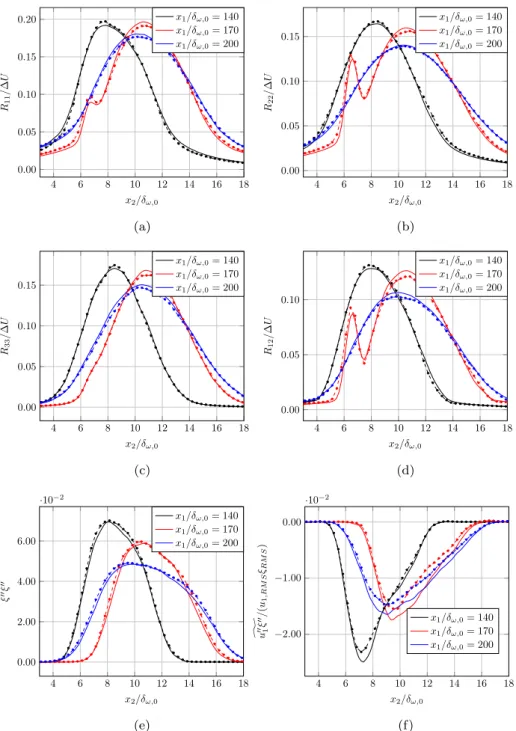
Fig. 21. Profiles of the Reynolds stress tensor components normalized by∆U together with the mixture fraction varianceξ˜′′_ξ′′_{and longitudinal component of the scalar} fluxu˜′′

1ξ′′at three abscissae, same symbols as those retained inFig. 17.

slight overestimate compared to the case where the effects of

κ

are considered. The region that extends from x1

/δ

ω,0

=

150

.

0

until the interaction with the reflected shock is characterized by a significant change of behavior and the values obtained with

κ ̸=

0 are larger than those obtained with

κ =

0. This

re-gion is characterized by strong pressure wave reflection from the upper limit of the computational domain. After the interaction with the reflected shock wave, the maxima of the TKE obtained with or without taking into account the bulk viscosity effects tend to become similar as the end of the computational domain is approached. It can be concluded that, in the absence of the second shock wave interaction and associated parasitic pressure waves issued from the top of the computational domain, the TKE levels

would be slightly underestimated if the effects of

κ

were not taken

into account. In an attempt to better understand the behavior of the TKE, the analysis of the main terms involved in its transport equation is now carried out.

The transport equation for the turbulent kinetic energy Kis

given by

∂

t(

ρ

K)

+

∇ ·

(

ρ˜

uK)

=

P

+

ε +

T

+

Π

+

Σ (12)

In this equation,Pis the production term,

ε

is the dissipation term,

T denotes the turbulent transport term,Πis the pressure–strain

term, and finallyΣthe mass flux term. The budget(12)is deduced

from the transport equation of the Reynolds tensor components:

∂

(

ρ

Rij)

∂

t

+

∂

(

ρ

_˜

ukRij)

∂

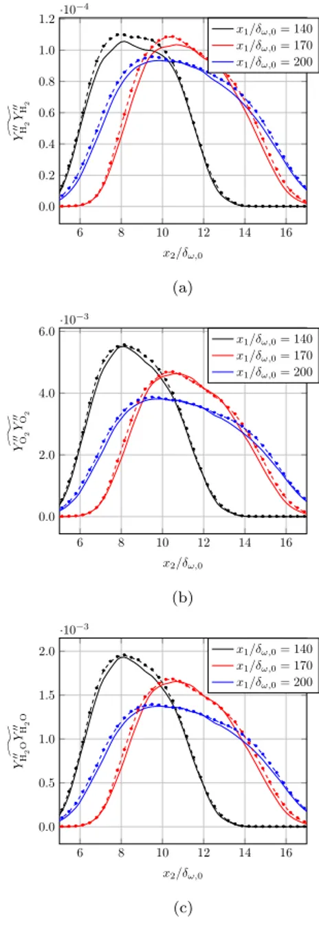
xk

Fig. 22. Profiles of the variances of chemical species mass fractions at three abscissae, same symbols as those retained inFig. 17. with ⎧ ⎪ ⎪ ⎪ ⎪ ⎪ ⎪ ⎪ ⎪ ⎪ ⎪ ⎪ ⎪ ⎪ ⎪ ⎪ ⎪ ⎪ ⎪ ⎨ ⎪ ⎪ ⎪ ⎪ ⎪ ⎪ ⎪ ⎪ ⎪ ⎪ ⎪ ⎪ ⎪ ⎪ ⎪ ⎪ ⎪ ⎪ ⎩ Pij= −ρ ( Rik∂˜uj ∂xk+Rjk ∂˜ui ∂xk ) , (a) εij= −τik′ ∂u′′ j ∂xk −τ ′ jk ∂u′′ i ∂xk, (b) Tij= − ∂ ∂xk(ρu ′′ iu ′′ ju ′′ k+P ′_u′′ iδjk+P′u′′jδik−τjk′u ′′ i −τ ′ iku ′′ j) , (c) Πij=P′∂ u′′ i ∂xj +P ′∂u ′′ j ∂xi, (d) Σij= ( u′′ i ∂ τjk ∂xk +u ′′ j ∂ τik ∂xk ) − ( u′′ i ∂P ∂xj +u ′′ j ∂P ∂xi ) (e) (14)

In the above set of equations, it has been chosen to split the pressure into a mean and a fluctuating part but it should be rec-ognized that there exist other ways to handle pressure terms in the second-order moment transport equations. Here, we are following the same procedure as the one previously considered by

Pantano et Sarkar [38]. However, it is acknowledged that, for other

conditions related, for instance, to transport modeling in turbulent premixed flames in the flamelet regime, keeping the instantaneous pressure can be a better choice since local flamelet relationships may provide relevant closures for the corresponding effects, see for instance Bray et al. [39] or Robin et al. [40].

The analysis of the main terms involved in the TKE transport equation is carried out at two distinct locations to infer the impact

of the volume viscosity.Figure 20shows that the most important

contributions are associated to the production and dissipation

terms. Their amplitude is found to be slightly smaller when

κ

is not

taken into account. The turbulent transport term is positive at the periphery of the mixing layer while it tends to be negative within the mixing layer. This quantity, which is larger in the case featuring

κ ̸=

0, removes energy from regions characterized by large

fluctuations levels to transfer it in regions characterized by lower

levels of TKE.Figure 20also shows that the contributions due to

pressure–strain and mass flux terms remain negligible compared to the others, for both cases.

Figure 21reports the distribution of the Reynolds stress com-ponents together with the variance of the passive scalar and the

scalar flux components for both cases

κ ̸=

0 and

κ =

0. The

three streamwise positions under consideration are representative

of the variations observed on the TKE profile reported inFig. 19.

The profiles of the Reynolds stress components show that the maxima of its diagonal components follow the trends reported in

Fig. 19.Figure 21(f), which displays the longitudinal evolution of the scalar flux component ˜u′′

1

ξ

′′

/

_(u

1,RMS

ξ

RMS), reveals that the

max-imum value of the correlation between the longitudinal velocity fluctuation and the scalar fluctuation is slightly underestimated when the effects of bulk viscosity are not considered.

Figure 22reports the variance of the mass fractions of chemical species present in the mixture. The hydrogen, which is

character-ized by the highest ratio

κ/µ

is the one that displays the largest

differences (up to approximately ten percent) between the two

cases, i.e.,

κ =

0 and

κ ̸=

0. The differences observed at the three

locations concern both the shape and maximum levels, which depend on the species under consideration. Indeed, it is found that the distribution of the profiles for all chemical species is slightly wider – indicating that the fluid is incorporated more markedly – when the effects of bulk viscosity are not taken into account, which leads to a reduction of fluctuations around the averaged value. A similar effect is observed when the convective Mach number values are increased [26,41].

5. Summary and conclusions

In the present manuscript, two- and three-dimensional nu-merical simulations of spatially-developing compressible mixing layers impacted by an oblique shock wave are conducted for a

convective Mach number Mc

=

0

.

48. The emphasis is placed on

the possible influence of the bulk viscosity on the mixing processes. Thus, a mixture of hydrogen and air is considered in conditions that are representative of experimental benchmarks relevant to high-speed flow combustion. In a first step of the analysis, two-dimensional computations of inert and reactive mixing layers are performed. A significant impact of the bulk viscosity is observed on the instantaneous flowfields while averaged quantities do not exhibit any remarkable modification. It is also worth noting that the reactive cases only display slight differences with respect to inert cases: this is especially true for the longitudinal evolutions of the vorticity thickness and turbulent kinetic energy. Three-dimensional simulations of inert mixing layers are subsequently conducted. The influence of the bulk viscosity is more visible in these three-dimensional cases: it tends to reduce the mixing layer growth rate compared to the case where it is not taken into account. The comparison is also performed in terms of higher-order statistical moments. This last part of the analysis shows that the bulk viscosity effects tend to amplify the velocity gradients at the boundaries of the mixing layer, and consequently favor the return to equilibrium. From the above synthesis of the obtained results, one may expect that refined large-eddy simulations (LES) may be rather sensitive to the consideration of bulk viscosity, while Reynolds-averaged Navier–Stokes (RANS) simulations, which are based on statistical averages, are not. One possible perspective of the present work concerns the filtering of the present dataset, which may provide further insights so as to assess this conclusion. Finally, from the present set of results, it is recommended to take the bulk viscosity effects into account especially when highly-resolved large-eddy simulations (LES) are considered.

Acknowledgments

The computations were performed using the High Performance Computing resources from the mésocentre de calcul poitevin and

from genci under allocations x20142a0912 and x20142b7251. The first author benefited from interesting discussions with Aimad Er-raiy. This work has been presented at the tenth International Con-ference on Computational Fluid Dynamics (Barcelona, July 2018). References

[1] U. Balucani, M. Zoppi, Dynamics of the Liquid State, Vol. 10, Clarendon Press, 1995.

[2] M.S. Cramer, Numerical estimates for the bulk viscosity of ideal gases, Phys. Fluids 24 (2012) 066102.

[3] G. Billet, V. Giovangigli, G. De Gassowski, Impact of volume viscosity on a shock–hydrogen-bubble interaction, Combust. Theory Model. 12 (2) (2008) 221–248.

[4] S. Chapman, T. Cowling, The Mathematical Theory of Non-uniform Gases, Cambridge University Press, 1970.

[5] A. Ern, V. Giovangigli, Volume viscosity of dilute polyatomic gas mixtures, European J. Mech. B 14 (5) (1995) 653–669.

[6] A. Ern, V. Giovangigli, Fast and accurate multicomponent transport property evaluation, J. Comput. Phys. 120 (1995) 105–116.

[7] A. Ern, V. Giovangigli,EGlibusers manual, 1996.

[8] G. Fru, G. Janiga, D. Thévenin, Impact of volume viscosity on the structure of turbulent premixed flames in the thin reaction zone regime, Flow Turbul. Combust. 88 (4) (2012) 451–478.

[9] M.S. Cramer, F. Bahmani, Effect of large bulk viscosity on large-Reynolds-number flows, J. Fluid Mech. 751 (2014) 142–163.

[10] F. Bahmani, M.S. Cramer, Suppression of shock-induced separation in fluids having large bulk viscosities, J. Fluid Mech. 756 (2014) 142–163.

[11] A.V. Chikitkin, B.V. Rogov, G.A. Tirsky, S.V. Utyuzhnikov, Effect of bulk viscosity in supersonic flow past spacecraft, Appl. Numer. Math. 93 (2015) 47–60. [12] C. Huete, A.L. Sánchez, F.A. Williams, Diffusion-flame ignition by shock-wave

impingement on a hydrogen/air supersonic mixing layer, J. Propul. Power 33 (2017) 256–263.

[13] R. Buttay, G. Lehnasch, A. Mura, Analysis of small-scale scalar mixing pro-cesses in highly under-expanded jets, Shock Waves 26 (2) (2016) 93–212. [14] R. Boukharfane, Z. Bouali, A. Mura, Evolution of scalar and velocity dynamics

in planar shock-turbulence interaction, Shock Waves 28 (2018) 1117–1141. [15] P.J. Martínez Ferrer, R. Buttay, G. Lehnasch, A. Mura, A detailed verification

procedure for compressible reactive multicomponent Navier–Stokes solvers, Comput. & Fluids 89 (2014) 88–110.

[16] J. Lin, C. Scalo, L. Hesselink, High-fidelity simulation of a standing-wave thermoacoustic–piezoelectric engine, J. Fluid Mech. 808 (2016) 19–60. [17] G.J. Prangsma, A.H. Alberga, J.J.M. Beenakker, Ultrasonic determination of the

volume viscosity of N2,CO,CH4,and CD2between 77 and 300 K, Physica 64 (2) (1973) 278–288.

[18] D. Bruno, V. Giovangigli, Relaxation of internal temperature and volume viscosity, Phys. Fluids 23 (2011) 093104.

[19] A. Ern, V. Giovangigli, Multicomponent Transport Algorithms, Vol. 24, Springer Science & Business Media, 1994.

[20] L. Monchick, E.A. Mason, Transport properties of polar gases, J. Chem. Phys. 35 (5) (1961) 1676–1697.

[21] A. Ern, V. Giovangigli,EGlib: A general-purpose fortran library for multi-component transport property evaluation. Technical report, ManualEGlib

Version, 2004.

[22] A.C. Hindmarsh, P.N. Brown, K.E. Grant, S.L. Lee, R. Serban, D.E. Shumaker, C.S. Woodward, Sundials: Suite of nonlinear and differential/algebraic equation solvers, ACM Trans. Math. Software 31 (3) (2005) 363–396.

[23] J.L. Ziegler, R. Deiterding, J.E. Shepherd, D.I. Pullin, An adaptive high-order hybrid scheme for compressible, viscous flows with detailed chemistry, J. Comput. Phys. 230 (20) (2011) 7598–7630.

[24] R. Boukharfane, F.H.E. Ribeiro, Z. Bouali, A. Mura, A combined ghost-point-forcing/direct-forcing immersed boundary method (IBM) for compressible flow simulations, Comput. & Fluids 162 (2018) 91–112.

[25] J.D. Ramshaw, Simple model for mixing at accelerated fluid interfaces with shear and compression, Phys. Rev. E 61 (5) (2000) 5339.

[26] P.J. Martínez Ferrer, G. Lehnasch, A. Mura, Compressibility and heat release effects in high-speed reactive mixing layers. Growth rates and turbulence characteristics, Combust. Flame 180 (2017) 284–303.

[27] C. Pantano, S. Sarkar, F.A. Williams, Mixing of a conserved scalar in a turbulent reacting shear layer, J. Fluid Mech. 481 (2003) 291–328.

[28] R.E. Mitchell, R.J. Kee, General-purpose computer code for predicting chemical-kinetic behavior behind incident and reflected shocks. Technical report, Sandia National Labs., Livermore, CA (USA), 1982.

[29] M. Ó Conaire, H.J. Curran, J.M. Simmie, W.J. Pitz, C.K. Westbrook, A compre-hensive modeling study of hydrogen oxidation, Int. J. Chem. Kinet. 36 (11) (2004) 603–622.

[30] R. Buttay, G. Lehnasch, A. Mura, Turbulent mixing and molecular transport in highly under-expanded hydrogen jets, Int. J. Hydrogen Energy 43 (17) (2018) 8488–8505.

[31] R. Buttay, L. Gomet, G. Lehnasch, A. Mura, Highly resolved numerical simula-tion of combussimula-tion downstream of a rocket engine igniter, Shock Waves 27 (4) (2017) 655–674.

[32] S.B. Pope, Turbulent Flows, Cambridge University Press, 2000.

[33] M. Brouillette, The Richtmyer-Meshkov instability, Annu. Rev. Fluid Mech. 34 (1) (2002) 445–468.

[34] Y. Yan, C. Chen, P. Lu, C. Liu, Study on shock wave-vortex ring interaction by the micro vortex generator controlled ramp flow with turbulent inflow, Aerosp. Sci. Technol. 30 (1) (2013) 226–231.

[35] C.D. Pierce, Progress-variable Approach for Large-eddy Simulation of Turbu-lent Combustion (Ph.D. thesis), Stanford University, 2001.

[36] L. Gomet, V. Robin, A. Mura, A multiple-inlet mixture fraction model for non premixed combustion, Combust. Flame 162 (2015) 668–687.

[37] H. Gonzalez, G. Emanuel, Effect of bulk viscosity on Couette flow, Phys. Fluids A 5 (5) (1993) 1267–1268.

[38] C. Pantano, S. Sarkar, A study of compressibility effects in the high-speed turbulent shear layer using direct simulation, J. Fluid Mech. 451 (2002) 329– 371.

[39] K. Bray, M. Champion, P. Libby, Premixed flames in stagnating turbulence. Part IV: a new theory for Reynolds stresses and Reynolds fluxes applied to impinging flows, Combust. Flame 120 (2000) 1–18.

[40] V. Robin, M. Champion, A. Mura, A second-order model for turbulent reactive flows with variable equivalence ratio, Combust. Sci. Technol. 180 (2008) 1707–1732.

[41] I. Mahle, Direct and Large-eddy Simulation of Inert and Reacting Compressible Turbulent Shear Layers (Ph.D. thesis), Technische Universität München, 2007.