is an open access repository that collects the work of Arts et Métiers Institute of
Technology researchers and makes it freely available over the web where possible.
This is an author-deposited version published in: https://sam.ensam.eu Handle ID: .http://hdl.handle.net/10985/11834
To cite this version :
Mernhaz FARZAM FAR, Anouar BELAHCEN, Paavo RASILO, Stéphane CLENET, Antoine PIERQUIN - Model Order Reduction of Electrical Machines with Multiple Inputs - Transactions on Industrial Applications - Vol. PP, n°99, p.1-6 - 2017
Any correspondence concerning this service should be sent to the repository Administrator : [email protected]
Abstract -- In this paper, proper orthogonal decomposition method is employed to build a reduced-order model from a high-order nonlinear permanent magnet synchronous machine model with multiple inputs. Three parameters are selected as the multiple inputs of the machine. These parameters are terminal current, angle of the terminal current, and rotation angle. To produce the lower-rank system, snapshots or instantaneous system states are projected onto a set of orthonormal basis functions with small dimension. The reduced model is then validated by comparing the vector potential, flux density distribution, and torque results of the original model, which indicates the capability of using the proper orthogonal decomposition method in the multi-variable input problems. The developed methodology can be used for fast simulations of the machine.
Index Terms--Electrical machines, Finite element methods, Interior permanent magnet machine, Model order reduction, Proper orthogonal decomposition.
I. INTRODUCTION
HE finite-element (FE) method (FEM) is a beneficial and powerful numerical tool in analyzing static or dynamical systems. However, the numerical simulations of real-life problems may face difficulties in design optimization and control due to the complexity of the system, computational high costs, and storage requirement [1]. In order to solve this problem, it is pertinent to use model order reduction (MOR) method such as proper orthogonal decomposition (POD), as one of the most common methods [2]. In this paper, the POD method has been employed to reduce the order of a nonlinear permanent magnet synchronous (PMS) machine with 3 inputs.
POD, also known as Karhunen-Loeve decomposition, principal components analysis, or the empirical eigenfunctions method, was originally developed in the field of structural dynamics [3]. However, nowadays, POD method has a wide range of application in various fields of engineering such as FE modelling [4], fault diagnosis [5], and modal analysis [6]. Moreover, this method is useful in reducing the order of both linear and nonlinear systems
This work was supported by the Academy of Finland under Grant13287395 and 274593.
M. Farzamfar is with the Department of Electrical Engineering and Automation, Aalto University, 02150 Espoo, Finland ([email protected]).
A. Belahcen is with the Department of Electrical Engineering and Automation, Aalto University, Finland and Department of Electrical Engineering, Tallinn University of Technology, Estonia ([email protected]).
P. Rasilo is with Laboratory of Electrical Energy Engineering, Tampere University of Technology, Tampere, Finland and the Department of Electrical Engineering and Automation, Aalto University, 02150 Espoo, Finland ([email protected]).
S. Clénét is with Univ. Lille, Arts et Métiers Paris Tech, EA 2697 - L2EP - Laboratoire d’Electrotechnique et d’Electronique de Puissance, F-59000 Lille, France ([email protected]).
A. Pierquin is with Univ. Lille, EA 2697 - L2EP - Laboratoire d’Electrotechnique et d’Electronique de Puissance, F-59000 Lille, France ([email protected]).
[10]. The key feature of POD method, as a projection method, is to achieve an optimal approximating subspace to a given set of data [11]. The choice of this data set indeed affects the reduced model results. Sirovich [12] introduced a convenient method, known as method of snapshots, to obtain this data set, or snapshots. The snapshots can be selected by solving the system via experiment or numerical simulation in time domain, frequency domain, or any other configuration. Therefore, the POD method is a data dependent method, which does not require a priori knowledge of the system behavior [13].
In this paper, we show that POD method can be used to study nonlinear electrical machines with multiple parameters. Three parameters are selected as the inputs of the machine: terminal current, angle of the terminal current, and rotation angle. The reduced model will be valid for any value of input into the parameter range. In Section II, we provide the basic required background of POD method and an application of this method in electrical machine. Section III is dedicated to the comparison of the original model and the approximated model obtained via the POD method. Finally, in Section IV, the conclusion of the work and the future research perspectives are presented [14].
II. PROPER ORTHOGONAL DECOMPOSITION
A. Numerical Concept of POD
In this section, we provide a brief introduction (see [13] for a more detailed discussion) of using POD method to reduce the order of a nonlinear system with m degrees of freedom (DoF). Assume that this system is defined by the following partial differential equation over some domain of interest [8]
( , , ,..., , )
t x xx x t
Y F Y Y Y (1) where Y is a state vector, subscripts x and t define partial differentiation, and the function F(·) captures the space-vector of system with predefined initial and boundary conditions. Furthermore, assume a scalar quantity y(x, t) to be a solution of the system, obtained by eigenfunction expansion techniques. 1 ( , ) n( ) n( ) n x t a t x
y (2)where the ϕn(x) is an orthogonal set of eigenfunctions and an(t) is the sequence of the configurations functions in association with the corresponding n( )x .
The basis functions n( )x can be generated by different methods such as Fourier series, Legendre polynomials, or Chebyshev polynomials. In this paper, however, the optimal POD basis functions (or POD modes) are built by implementing singular value decomposition (SVD) for a given data set or snapshots. To get the snapshots, let’s assume the mentioned system is solved at n exclusive times,
Model Order Reduction of Electrical Machines
with Multiple Inputs
M. Farzam Far, A. Belahcen, P. Rasilo, S. Clénet, A. Pierquin
frequencies, or other configurations. These solutions are then stored in matrix Sn, called a snapshot matrix, with the size of (m×n) and rank of k. The SVD decomposes the snapshot matrix as
n *
S UΣV (3) where * stands for the transpose of a vector or matrix. The matrices U with the size of m×m and V with the size of n×n are orthonormal matrices containing the left-singular vectors and right-singular vectors, respectively. Σ is a m×n rectangular diagonal matrix with singular values i as the diagonal entries. The singular values are ordered in such a way that 12 ... 0. According to [3], the POD modes are equal to the left-singular vectors of Sn.
After obtaining the POD modes, the question is how many of these modes we should take into account to create a lower-rank approximation of the snapshot matrix while accurately capturing the behavior of the system. The key to this question is the oriented energy distribution of the vector set of the matrix. The SVD of the snapshot matrix provides valuable information regarding this oriented energy distribution. The energy of a vector sequence equals to the energy in its singular spectrum 12,...,2p (p=min(m, n)) and the whole energy of the system is the sum of the squares of all the singular values [3]. Therefore, the POD modes can be optimized with respect to energy content in a least squares sense.
Considering the energy of each mode, one can determine the required number of modes (l, 1≤ l≤ k) by the following criterion to be less than a desired error ε [15]
2 r 2 =1 = +1 n k j j i j i l y y
(4)where y is the unique solution to (1) and yr is the POD approximation of y, defined as r 1 ( , ) l j j i i i y y
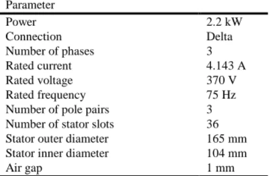
(5) B. Application of POD in Electrical MachineIn this section we focus on the application of the POD in order reduction of the model of an electrical machine with multiple inputs. In this work, the FEM is used to simulate a 2.2 kW interior magnet PMS machine. Second order elements are used for the simulation. Some of the machine characteristics and its FE mesh are presented in Table I and Fig. 1, respectively.
TABLEI PARAMETERS OF THE MACHINE
Parameter Power 2.2 kW Connection Delta Number of phases 3 Rated current 4.143 A Rated voltage 370 V Rated frequency 75 Hz
Number of pole pairs 3
Number of stator slots 36
Stator outer diameter 165 mm
Stator inner diameter 104 mm
Air gap 1 mm
Fig. 1. Computational domain (in cm) and FE mesh of the test machine.
The behavior of the machine is defined in the 2-D cross section of the machine using the magnetic vector-potential formulation [16]. The iron losses are neglected and the non-linearity of the iron is taken into account with nonlinear single valued material properties. By means of the Galerkin method, one can obtain the matrix format of the discretized magnetostatic field equation of the nonlinear machine in the form of [17]
( )
S u u f (6) where S is the sparse stiffness matrix of the system, u is the vector containing the potentials of the nodes, and f is the source vector. In order to solve the system equation (6) for any desired u, a Newton-Raphson iteration scheme is employed to deal with the nonlinearity of the equation. By defining the residual matrix r as r = Su – f, the Newton-Raphson iteration can be written as in (7). The iteration starts from an initial value u0 and continues until the solution ui is obtained, under a certain convergence criterion [18].
1
1 ( 1)
i i i
u u J r u (7) where J is the Jacobian matrix
( i) i i S u J u (8) The aim of this paper is to apply the POD method to the model with multiple variables as input. We consider the magnitude of the terminal current (i), the angle of the terminal current (α), and the electrical rotation angle of the machine (θ) as three inputs of the machine. Therefore, (6) will be dependent on these three variables.
To reduce the order of the model, vector u is approximated to a lower-rank vector ur, which is to say
r
u Φu (9) where the matrix Φ is constructed by the method of snapshots (as discussed in the previous section). To fulfill the purpose of this paper, the snapshot matrix is defined by varying the three defined inputs one at a time. The system is solved for 11 terminal currents equally distributed between zero and the rated current, and the current angle and the electrical rotation angle, each, vary from 0 to 180 electrical degrees with 10 degree angle step. The 3564 computed solutions are stored in the snapshot matrix Sn (1379×3564). Using any scientific software packages, such as MATLAB, one can easily compute the SVD of Sn. The energy (the square of singular values) of the first 100 POD modes are plotted in Fig. 2. According to this figure, the energy of the
modes decay exponentially in spite of the nonlinearity of the machine. This is due to the fact that the first states contain most of the energy of the system [19].
Fig. 2. The energy spectrum of the first 100 POD modes.
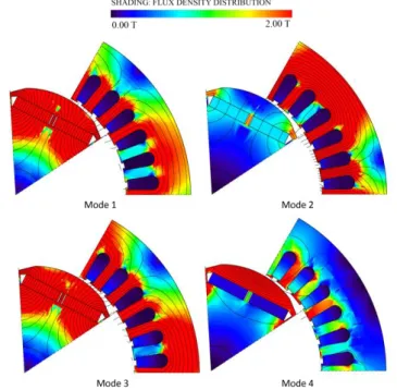
Now we shall determine the required number of the left-singular vectors to be considered as the POD modes. Looking at Fig. 2, it can be observed that the first four POD modes have the highest singular values and, therefore, most of the system energy. These POD modes are shown in Fig. 3. It is worth mentioning that the POD modes do not represent the original model, but their combination through a POD reconstruction provides the most energetic behavior of the system [20], [21]. Moreover, due to the data dependency of the POD method, it is not possible to provide a general physical interpretation of the POD modes, particularly in nonlinear systems [3].
Fig. 3. POD modes of the machine.
The first four POD modes captures a considerable portion (about 93%) of the energy of the system. However, reconstructing the approximated POD model with only these POD modes will not results in a satisfying accuracy (This is shown in (Section IV. A)). This suggests that, in the case of a nonlinear system with multiple inputs, an additional condition is required to select the required number of POD modes than predicting this number merely by comparing the energy of the POD modes visually. Hence, the criterion mentioned in (4) is employed to select the required number of POD modes. The value of ε in this equation is chosen with
respect to the desired accuracy between the original model and its approximation; indeed, the smaller the chosen value is, the more precise the POD model will be. In this work, for an accurate approximation, we set ε to 2×10⁻⁵. With this consideration, the required number of POD modes is 63.
Finally, the approximated POD model can be written in the form of
r r r
S u f (10)
where Sr = Φ*S(Φur)Φ and f r = Φ*f. As mentioned before, S is a sparse matrix; whereas, Sr is a full matrix but it has a smaller size than S. Therefore, the rank of the POD model in (10) is much smaller than the rank of FE model in (6). Here also due to the nonlinearity of the system, the reduced system equation (10) is solved by applying Newton-Raphson method as following
r r r 1 r
1 ( ) ( 1)
i i i
u u J r u (11) where in the reduced case the residual (rr) and Jacobian Jr matrices would be r r r r r S u f (12) r r r r ( ) * S u J Φ JΦ u (13)
III. RESULTS AND DISCUSSION
In this section, the accuracy of the low-rank approximated POD model is examined by comparing the field results of the original model and the approximated model. The comparison is performed at two stages; first, for a local comparison, the two models are solved and compared at two randomly selected operation points and in the second stage, for an average error, the original model and approximated model are solved for 150 unique and randomly chosen input operation points and a global error formula is applied to compute the error of these results. The following sub-sections present each of these two stages in details.
A. Local Error
The approximated POD model is built in two different configurations. In the first configuration, the reduced model is reconstructed by taking into account the first 4 POD modes (according to the singular values), and in the second configuration, the first 63 POD modes (obtained from (4), ε = 2×10⁻⁵) are considered in building the reduced model. Thereafter, the original model and the POD approximation model are solved at two operation points, for each of these configurations. These two points are randomly chosen from the working interval of the PM machine and are assumed to be
Case 1: terminal current i = 1.3 A, angle of the terminal current α = 12.5 º, electrical rotation angle of the machine θ = 115º.
Case 2: terminal current i = 4.1 A, angle of the terminal current α = 35 º, electrical rotation angle of the machine θ = 150º.
The accuracy of the POD reduced model is then examined by comparing the vector-potentials of the original model (u) with its low-rank approximation (Φur), for each case and configuration. The error δ between the vector-potential of the two models is measured by the following equation.
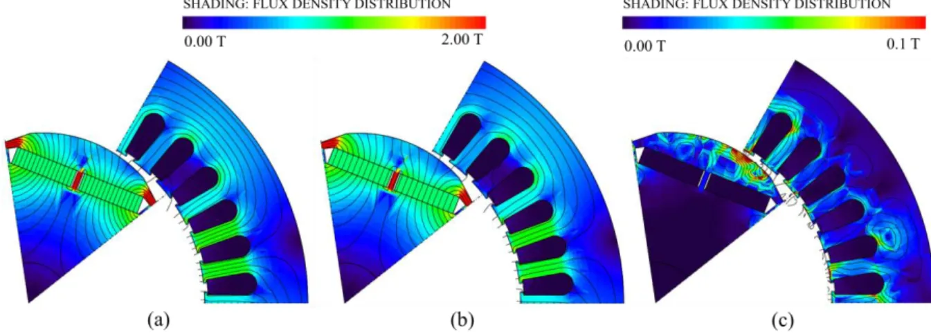
Fig. 5. Flux density distribution of Case 2 obtained from (a) original model, (b) POD approximated model, and (c) their difference
r
Φu
u
u
(14)In the first configuration, in which the system is retained by only 4 POD modes, the percent error is 9.5 % for Case 1 and 23.88 % for Case 2. However, in the second configuration, 63 POD modes are chosen to rebuild the system, the value of δ is 13×10-3 % for Case 1 and this error in Case 2 is 2.2×10⁻³ %. By comparing the figures from these two configurations, we can conclude that in predicting the required number of POD modes, a better accuracy is guaranteed when using (4). Therefore, we select the first 63 left-singular vectors as the POD modes in the rest of the evaluations in this paper.
Furthermore, the flux density distribution and the airgap torque of the original model and its approximation are computed. The results of flux density distribution of both models for Case 1 are shown in Fig. 4 (a), (b) and the results of Case 2 are shown in Fig. 5 (a), (b). Since the flux
distribution of the original and POD models are highly similar and no vivid difference can be observed visually, the difference between the flux density distributions of two models are plotted in Fig. 4. (c) and Fig. 5. (c) for each case. According to Fig. 4. (c) and Fig. 5. (c), the maximum flux density difference between the original model and the low-ranked approximated model is less than 100 mT for Case 1 and less than 30 mT for Case 2, which indicate the accuracy of the approximated model.
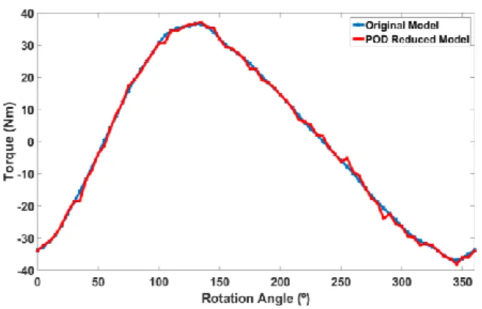
Fig. 6 presents the torque results of the original model and the POD approximated models. The torque is computed by considering the input current of 4.1 A, the current angle of 25º, and varying the rotational angle from zero to 360 electrical degree. The reason of choosing the mentioned value of input current and its angle is to compare the results of the reduced model at operating points, which are not included in the snapshot matrix.
Fig. 6. Air-gap torque computed by the original model and the reduced POD model at different angular positions of the rotor.
The similarity between the torque results of the two models shows the POD model capability to approximate the original model. It should be noted that the snapshot matrix was selected for rotation angle from the interval [0, 180] degree. However, the torque results (Fig. 6) are plotted for the interval [0, 360]. This suggests that POD based models often have the ability of estimating the system outside of the interval where the snapshots are defined [8].
B. Average Relative Error
Previously, the original model and its approximation have been compared at specific input values. In order to test how well the reduced model can represent the original model at any desired input operation point, an average relative error is defined as [22] r av-rel 0
1
N i i i iU
U
E
N
U
(15)where N is the number of input operating points. Ui and Uir are the output quantities associated with the i-th input, obtained from the original model and the POD approximated model, respectively.
In this work, the average relative error is calculated for vector potentials results of the original model and its approximation. For this purpose the vector potential is solved for 150 different samples of the input operating points (N = 150). Each of these N samples are unique and randomly chosen from the working interval of the machine (i ϵ [0, 4.14] A, α ϵ [0, 180] º, θ ϵ [0, 180] º). These samples are then substituted in (10) to obtain Eav-rel. The obtained error for the vector potential is 2.5 %.
The two models are also compared in term of computational time. The average time required to solve the system equation is about 0.18 s for the original model and 0.09 s for the POD approximated model, which implies the capability of POD in reducing the size and the computational time of a high order system.
IV. CONCLUSION
The POD projection method, combined with the Galerkin method, is one of the most efficient methods in reducing the complexity and the computational costs of high-dimensional systems of equations. This work presented a successful attempt to implement the POD method to reduce the model order of a PMS machine with multiple inputs. The achieved accuracy of the vector potential, flux density distribution,
and torque results of the POD reduced model is an indicator that the reduced model presents the original model well on all the operating range of the machine. This accuracy, however, depends on various factors such as the size and the selection of snapshot matrix or the number of POD modes.
It is shown that the POD based model can predict the system even outside of the working domain where the snapshot matrix is defined. Moreover, comparing this work with [19], one can conclude that the number of input variables affects the size of snapshot matrix and the required POD modes. A system with more input variables requires a larger snapshot matrix as well as a greater number of POD modes.
The main advantage of POD is reducing the size and the computational time of a high order model. POD can be performed in two stages, at offline and online operation. In the offline operation, the method of snapshots is applied to construct the POD reduced model; in the online operation, the output results of the system is estimated via POD model for any input of interest. This ability can be of great help in real-time control of electrical machine by decreasing the online-required computational time and memory allocation in the microcontrollers. Therefore, POD can be as a replacement to time-step analyses or applied to reduce the computational burden of real-time problems. The possibility of applying the method in analyzing the real-time system will be investigated in future papers.
V. REFERENCES
[1] M. Sudheer Kumar, S. Harish, A.Dhanamjay Apparao, "Design of PID controller via novel model order reduction technique," IJARCCE, vol. 4, pp. 278-281, May. 2015.
[2] T. Henneron, S. Clenet, "Model order reduction of non-linear magnetostatic problems base on POD and DEI methods," IEEE Trans.
Magn., vol. 50, no.2, pp.33-36, Feb. 2014.
[3] G. Kerschen, J. C. Golinval, A. F. Vakakis, L. A. Bergman, "The method of proper orthogonal decomposition for dynamical characterization and order reduction of mechanical systems: an overview," Nonlinear Dynamics, vol. 41, pp. 147-169, 2005. [4] V. Lenaerts, G. Kerschen, J. C. Golinval, "Identification of a
continuous structure with a geometrical non-linearity. Part II: Proper orthogonal decomposition," Journal of Sound and Vibration, vol. 262, no. 4, pp. 907-919, May, 2003.
[5] P. De Boe, J. C. Golinval, "Principal component analysis of a piezo-sensor array for damage localization," Structural Health Monitoring, vol. 2, no. 2, pp. 263-277, May, 2013.
[6] B. F. Feeny., "On proper orthogonal coordinated as indicators of modal activity," Journal of Vibration and Acoustics, vol. 255, no. 5, pp. 157-160, 2002.
[7] P. Holmes, J.L. Lumley, G. Berkooz, C.W. Rowley. (2012, June).
Turbulence, Coherent Structure, Dynamical System and Symmetry.
(2nd ed.). Cambridge: Cambridge University Press. Available: http://dx.doi.org/10.1017/CBO9780511919701 [10 March 2016]. [8] E. Shlizerman, E. Ding, M.O. Williams, J. N. Kutz, "The proper
orthogonal decomposition for dimensionality reduction in mode-locked lasers and optical system," International Journal of Optics, vol. 2012, Jun. 2011.
[9] M. Hinze, S. Volkwein, "Proper orthogonal decomposition surrogate models for nonlinear dynamical systems: error estimation and suboptimal control," in Dimension reduction of large-scale systems, vol. 45, Ed. Berlin: Springer Berlin Heidelberg, 2005, pp. 261-306. [10] A. Verhoeven, M. Striebel, J. Rommes, E. J. W. Maten, T. Bechtold,
"Proper orthogonal decomposition model order reduction of nonlinear IC models," in Progress in industrial mathematics at ECMI 2008, vol. 15, Ed. Berlin: Springer Berlin Heidelberg, 2010, pp. 441-446. [11] M. Rathinam, L. R. Petzold, "A new look at proper orthogonal
decomposition," SIAM J. NUMER. ANAL., vol. 41, no. 5, pp. 1893-1925, 2003.
[12] L. Sirovich, "Turbulence and the dynamics of coherent structures. I-III, " Quart. Appl. Math., vol. 45, no. 3, pp. 561–590, Oct. 1987.
[13] R. Pinnau, "Model reduction via proper orthogonal decomposition," in Model order reduction, Ed. Berlin: Springer Berlin Heidelberg, vol. 13, 2008, pp. 95-109.
[14] M. Farzamfar, A. Belahcen, P. Rasilo, S. Clénet, A. Pierquin, “Model order reduction of electrical machines with multiple inputs,” XXXII
international Conference on electrical Machines, 4-7.9.2016,
Lausanne, Switzerland.
[15] S. Volkwein. Proper orthogonal decomposition: Applications in optimization and control. Lecture Notes. [Online]. Available: math.uni-konstanz.de
[16] A. Arkkio, "Analysis of induction motors based on the numerical solution of the magnetic field and circuit equations," Ph.D. dissertation, Dept. Elect. Eng., Helsinki Univ. of Technology, Espoo, Finland, 1987.
[17] M. T. Holmberg, "Three-dimensional finite element computation of eddy currents in synchronous machines," Ph.D. dissertation, Dept. Elect. Eng., Chalmers Univ., Goteborg, Sweden, 1998.
[18] E. Dlala, A. Arkkio, "General formulation for the Newton-Raphson method and the fixed-point method in finite-element programs," in
Electrical Machines (ICEM), 2010 XIX Int. Conf., Rome, 2010, pp.
1-5.
[19] M. Farzamfar, P. Rasilo, F. Martin, A. Belahcen, "Proper orthogonal decomposition for order reduction of permanent magnet machine model," in Electrical Machine and systems (ICEMS), 18th Int. Conf., 2015, pp.1945-1949.
[20] W. Haase, M. Braza, A. Revell, "The IMFT circular cylinder experiment," in Desider- a European effort on hybrid Rans-Les
modelling, Ed. Berlin: Springer Berlin Heidelberg, vol. 103, 2009, pp.
97.
[21] K. E. Meyer, D. Cavar, J. M. Pedersen, "POD as a tool for comparison of PIV and LES data," in Particle Image Velocimetry, 7th Int.
Symposium, 2007.
[22] O. Lass, S. Volkwein, "POD Galerkin schemes for nonlinear elliptic-parabolic systems," SIAM J. Sci. Comput., vol. 35, no. 3, pp. 1271-1298, May, 2013.
VI. BIOGRAPHIES
Mehrnaz Farzamfar was born in Shiraz, Iran, in 1986. She received the
B.Sc. degree in electrical engineering from Kerman University, Iran, and the M.Sc. (Tech) degree in electrical engineering from Aalto University,
Espoo, Finland, in 2009 and 2014, respectively. She is currently working toward the D.Sc. degree in Aalto University, Espoo, Finland.
Anouar Belahcen (M13-SM15) received the M.Sc. (Tech.) and Doctor
(Tech.) degrees from Helsinki University of Technology, Finland, in 1998, and 2004, respectively. He is now Professor of electrical machines at Tallinn University of Technology, Estonia and Professor of Energy and Power at Aalto University, Finland. His research interest are numerical modeling of electrical machines, magnetic materials, coupled magneto-mechanical problems, magnetic forces, magnetostriction, and fault diagnostics.
Paavo Rasilo received his M.Sc. (Tech.) and D.Sc. (Tech.) degrees from
Helsinki University of Technology (currently Aalto University) and Aalto University, Espoo, Finland in 2008 and 2012, respectively. He is currently working as an Assistant Professor at the Department of Electrical Engineering, Tampere University of Technology, Tampere, Finland. His research interests deal with numerical modeling of electrical machines as well as power losses and magnetomechanical effects in soft magnetic materials.
Stéphane Clénet received an engineering degree in 1990 and a Ph.D
degree in 1994 both from the Institut National Polytechnique de Toulouse. From 1994 till 2002 he was Assistant Professor with the Electrical Engineering department of the University of Lille. Since September 2002 he is professor at the Ecole Nationale Supérieure d’Arts et Métiers. He teaches courses on electrical machines and power electronics. His research concerns the numerical modelling of electromagnetic devices working at low frequency.
Antoine Pierquin received the Bachelor of mathematics and the M.Sc.
degree in scientific computing from Université Lille 1 respectively in 2009 and 2011, then the Ph.D. degree in electrical engineering from Ecole Centrale de Lille in 2014. He is currently a member of the Laboratoire d’Electrotechnique et d’Electronique de Puissance (L2EP), Lille, France. His research interests include model order reduction, coupling and optimization methods in electrical engineering.