Auditory frequency processing during wakefulness and sleep
par Ramona Kaiser
Département de psychologie Faculté des arts et des sciences
Université de Montréal
Thèse présentée à la Faculté des études supérieures en vue de l’obtention du grade de
Philosophiæ Doctor (Ph.D.) en psychologie
Décembre, 2017
Faculté des études supérieures
Cette thèse intitulée:
Auditory frequency processing during wakefulness and sleep
présentée par: Ramona Kaiser
a été évaluée par un jury composé des personnes suivantes: Nadia Gosselin Président-rapporteur Marc Schönwiesner, Directeur de recherche Annelies Bockstael Membre du jury
Marc Pell Examinateur externe
Thèse acceptée le 10 mai 2018
serait un rêve devenu réalité pour plusieurs. Pendant des décennies, cette idée a été rejetée en se basant sur la supposition que le cerveau endormi ne répond pas et est plutôt isolé. Par contre, quelques études démontrent que de l’information auditive pourrait être perçue et traitée pendant le sommeil, et que même de la nouvelle information pourrait être acquise. Toutefois, très peu est connu au sujet du type d’information qui peut être traitée, et si les étapes de traitement durant le sommeil sont comparables à celles effectuées pendant l’éveil. Le but de cette thèse est d’investiguer le traitement de fréquences auditives pendant le sommeil relativement à l’éveil. Tout au long de cette thèse, l’adaptation est utilisée pour vérifier le traitement fréquentiel (i.e., l’adaptation réfère à une réduction en activation corticale pour un signal prolongé ou répété). Nous avons testé la possibilité de modifier le traitement fréquentiel cortical par l’écoute de musique filtrée pendant l’éveil, ainsi que l’exposition à du bruit filtré pendant une nuit complète de sommeil. Le filtre utilisé est un filtre coupe-bande qui enlève certaines fréquences du signal. De plus, le traitement d’information fréquentielle a été testé pendant une nuit complète de sommeil. Les résultats montrent que l’écoute de musique filtrée pendant plusieurs jours induit des changements au traitement fréquentiel cortical par rapport au filtre appliqué. Des changements similaires ont été détectés après une nuit d’exposition au bruit filtré, ce qui indique un haut niveau de perception et de traitement d’information du cerveau endormi. Par contre, aucune différence en réponse fréquentielle spécifique n’a pu être détectée pendant le sommeil, ce qui indique que l’adaptation pourrait fonctionner différemment pendant le sommeil et l’éveil.
Mots-clés: Sommeil, traitement auditif, traitement fréquentiel, adaptation, filtre coupe-bande.
For decades this idea has been rejected based on the assumption that the sleeping brain is rather unresponsive and isolated. However, a small number of studies demonstrate that auditory information could be perceived and processed during sleep, and that even new information could be acquired. It is still unknown which kind of information can be processed, and whether processing steps performed during sleep are comparable to those performed during wakefulness. The aim of this thesis is to investigate the processing of auditory frequency information during sleep relative to wakefulness. Throughout this thesis frequency processing was measured via adaptation. Adaptation refers to a reduction in cortical activation for a prolonged or repeatedly presented signal. We tested the possibility to alter cortical frequency processing via notched music listening during wakefulness, as well as via notched noise exposure during whole night sleep (i.e., notched-music and notched-noise are sound signals from which certain frequencies have been removed). Furthermore the processing of frequency information was tested throughout whole night sleep. Results show that several day long notched-music listening induces changes in cortical frequency processing relative to the applied notch. Similar changes were detected after one night of notched-noise exposure, indicating a higher level of auditory information processing of the sleeping brain. However no differences in frequency processing could be detected during sleep, indicating that adaptation might function differently during sleep relative to wakefulness.
Keywords: Sleep, Auditory processing, Frequency processing, Adaptation, Notch.
Abstract iv
Le table des matières v
La liste des figures ix
La liste des tableaux x
La liste des sigles et des abréviations xi
CHAPITRE 1: INTRODUCTION 1
1.1. Sleep ...1
1.2. Sleep and Auditory processing ...3
1.3. Auditory frequency processing ...4
1.4. Research method: EEG ...6
1.4.1. General information ...6
1.4.2. Event related potentials (ERPs) ...7
1.4.3. ERPs and Sleep ...9
1.5. Research background ...12
1.5.1. General information ...12
1.5.2. Frequency specificity, Adaptation, and Amplitude modulation ...14
CHAPITRE 2: THE EFFECT OF NOTCHED MUSIC LISTENING (ARTICLE 1) 17 2.1. Introduction ...17
2.2. Methods ...20
2.2.1. Participants ...21
2.2.2. Stimuli and Materials ...21
2.2.2.1. Music listening period ...21
2.2.2.2b Amplitude modulation test ...23
2.2.3. Design ...23
2.2.4. Procedure and Data acquisition ...24
2.2.4.1. Adaptation test ...25
2.2.4.2. Amplitude modulation test ...25
2.2.5. Data processing ...25
2.2.5.1. Music listening period ...25
2.2.5.2. Adaptation test ...26
2.2.5.3. Amplitude modulation test ...27
2.3. Analyses and Results ...30
2.3.1. Music listening ...30
2.3.2. Adaptation test ...30
2.3.2a Notch range activation ...30
2.3.2b Frequency activation ...33
2.3.3. Amplitude modulation test ...35
2.3.3a Notch range activation ...35
2.3.3b Frequency activations ...37
2.4. Discussion and Conclusion ...38
2.4.1. Comparison of EEG tests...39
2.4.2. Result 1: Induced changes in cortical frequency processing ...40
2.4.3. Result 2: Increased activation for frequency in within-notch range ...41
2.4.4. Result 3: Increased activation for frequencies in both notch ranges ...43
3.1. Introduction ...47
3.2. Methods ...50
3.2.1. Participants ...50
3.2.2. Material ...51
3.2.3. Design ...51
3.2.4. Procedure and Data acquisition ...52
3.2.5. Data processing ...53
3.3. Analyses and Results ...57
3.3.1. Frequency processing during wakefulness ...57
3.3.2. Frequency processing during sleep ...59
3.3.3. Differences in frequency processing between wakefulness and sleep ...60
3.4. Discussion ...62
3.4.1. Result 1: Frequency specific responses during wakefulness and sleep ...63
3.4.2. Result 2: Frequency specific responses across wakefulness and sleep ...65
CHAPITRE 4: AUDITORY PLASTICITY INDUCED DURING SLEEP (ARTICLE 3) 68 4.1. Introduction ...68
4.2. Methods ...72
4.2.1. Participants ...72
4.2.2. Stimuli and Material ...73
4.2.2.1. Night recording ...73
4.2.2.2. Test recordings ...74
4.2.3. Design ...75
4.2.4. Procedure and Data acquisition ...75
4.2.5. Data processing ...77
4.2.5.1. Night recording ...77
4.2.5.2. Test recordings ...78
4.3. Analyses and Results ...81
4.3.1. Night recording ...81
4.3.2. Test recordings ...82
4.3.2.1. Notch range activations ...82
4.3.2.1a Notch range differences ...82
4.3.2.1b Notch range mean ...83
4.3.2.2. Frequency activations ...84
4.4. Discussion and Conclusion ...86
4.4.1. Result 1: Rapidly induced effect of notched-noise exposure ...86
4.4.2. Result 2: Increased activation for the within-notch range ...89
4.4.3. Result 3: Effect limited to lowest frequency in the within-notch range ...90
CHAPITRE 5: GENERAL DISCUSSION 93 5.1. Notched sound exposure ...93
5.2. Frequency processing during sleep ...97
5.3. The impact of sleep on EEG measures ...99
BIBLIOGRAPHIE 102
Figure 2.1: Graphical display of frequency composition...22
Figure 2.2: Adaptation test: Grand average ERPs. ...28
Figure 2.3: Amplitude modulation test: Mean FFT. ...29
Figure 2.4: Adaptation test: Participant data for within-notch range across test sessions. ...32
Figure 2.5: Adaptation test: Notch range activations across test sessions. ...32
Figure 2.6: Adaptation test: Frequency activations. ...34
Figure 2.7: Amplitude modulation test: Notch range differences across test sessions per group. ...36
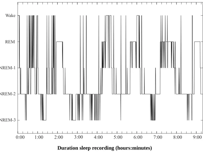
Figure 3.1: Hypnogram. ...55
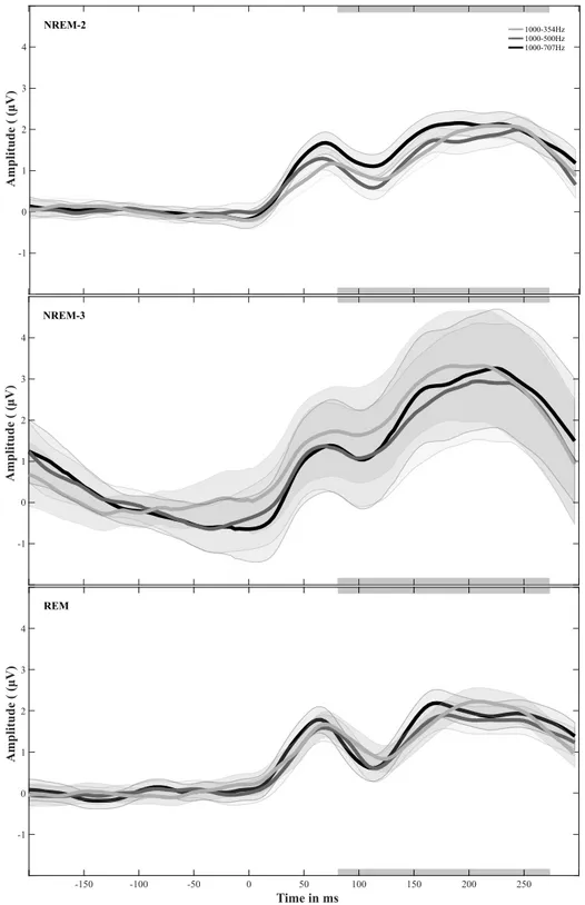
Figure 3.2: Grand average ERPs during sleep. ...56
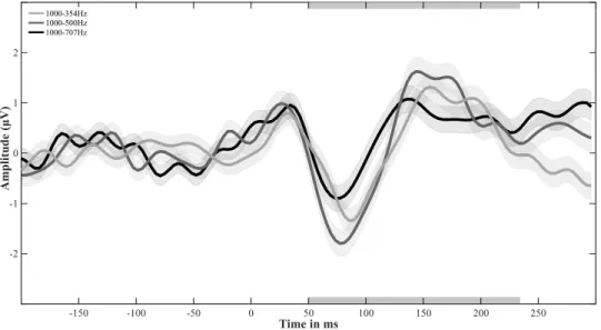
Figure 3.3: Grand average ERPs during wakefulness. ...57
Figure 3.4: Probe tone responses during sleep. ...59
Figure 3.5: Probe tone responses during sleep and wakefulness. ...61
Figure 4.1: Graphical display of frequency composition. ...75
Figure 4.2: Grand average ERPs. ...80
Figure 4.3: Mean notch range activations across test sessions. ...84
Figure 4.4: Frequency activations. ...85
Table 2.1: Amplitude modulation test: Frequency activations. ...38
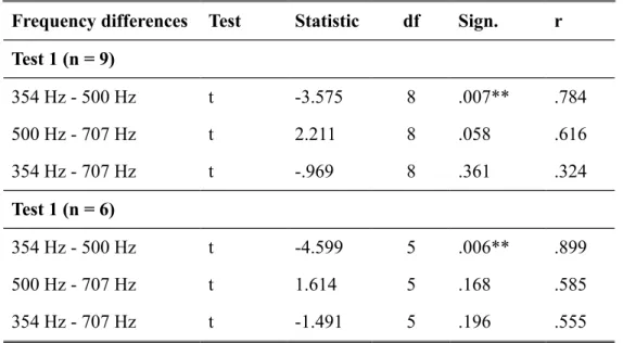
Table 3.1: Probe tone responses during wakefulness. ...58
Table 3.2: Probe tone responses during sleep and wakefulness. ...60
Table 3.3: Probe tone responses during REM sleep and wakefulness. ...62
AD Adaptation test; Performed in notched-music listening study (Chapitre 2) AM Amplitude modulation test; Performed in notched-music listening study
(Chapitre 2)
dB HL Decibel Hearing Level
dB SPL Decibel Sound Pressure Level
EEG Electroencephalography, Neuroimaging technique ERP Event related potential
fMRI Functional Magnetic Resonance Imaging, Neuroimaging technique Hz Hertz; Unit for frequency
MEG Magnetoencephalography; Neuroimaging technique REM Rapid eye movement sleep
NREM Non-rapid eye movement sleep
NREM-1 Non-rapid eye movement sleep – Sleep stage 1 NREM-2 Non-rapid eye movement sleep – Sleep stage 2 NREM-3 Non-rapid eye movement sleep – Sleep stage 3
N1 ERP component, Negative deflection of ERP waveform, around 100 ms after event onset
P2 ERP component; Positive deflection of ERP waveform, around 200 ms after event onset
INTRODUCTION
1.1. Sleep
“Sleep is the intermediate state between wakefulness and death; wakefulness being regarded
as the active state of all the animal and intellectual functions, and death as that of their total suspension.”
(Macnish, 1834; in Pelayo & Dement, 2017).
As indicated in this early definition, sleep has been considered a passive state in the beginning of sleep research. No clear differentiation was made between sleep and other states of low or no consciousness, like for example, coma or hibernation (Pelayo & Dement, 2017). Although the number of studies investigating sleep has increased tremendously over the last years, still little is known about its function and mechanisms (Walker & Stickgold, 2006). It is evident that, within a day, the human brain cycles through different levels of activity and arousal ranging from wakefulness to sleep. Sleep itself can be divided into rapid eye movement (REM) sleep and non-REM (NREM) sleep. Within one night NREM sleep and REM sleep interchange within sleep cycles. The length of sleep cycles, the average sleeping time, as well as the NREM-REM sleep ratio change throughout lifetime. For a healthy young adult a normal sleep night consists of about 75% - 80% NREM sleep and 20% - 25% REM sleep. Short periods of wakefulness may also occur during an average night sleep.
Normal sleep begins with a NREM sleep period and the first REM sleep period might occur as early as 80 minutes after sleep onset. Thereafter NREM and REM sleep periods alternate in cycles of about 90 minutes, however REM sleep periods tend to become longer throughout the night (Carskadon & Dement, 2017).
Theories about dreaming and sleep can be dated back to the earth’s earliest civilizations (Barbera, 2008). First research on sleep is tightly linked to the development of the Electroencephalography (EEG) method by Hans Berger in 1929 to measure electrical brain activity in humans. The EEG method allowed, for the first time, to perform sleep measurements with little or no disturbance for the sleeper (for a detailed historical review on sleep research see Dement, 1998). Today’s sleep research requires, at least, the application of EEG, electromyography (EMG), and electrooculography (EOG), which, in combination, are essential to estimate the sleep onset and to identify sleep stages and sleep cycles (for an overview on sleep staging see Hirshkowitz, 2017; see also Keenan & Hirshkowitz, 2017). Polysomnography, which implies measures like, for example, leg movements, the airflow during respiration, or electrocardiography (ECG), can be applied additionally to test for indications of sleep disorders or abnormalities (Mendelson, 1987). The identification of sleep stages is based on predefined norms. The first standardized classification system for human sleep was developed by Rechtschaffen and Kales in 1968. Their system defined seven separate sleep stages and was applied for decades worldwide. In 2007 the American Academy of Sleep Medicine (AASM) introduced, not without controversy, a new guideline for sleep research (Carskadon & Dement, 2017). Following the 2007 guideline NREM sleep is divided into three stages, stage 1 (NREM-1), the onset period of sleep which is often also referred to as ‘drowsiness’, stage 2 (NREM-2), and stage 3 (NREM-3), which is also known to as slow wave
sleep (SWS) due to the dominance of delta activity, that is slow oscillating high amplitude waves, during this sleep stage (Carskadon & Dement, 2017). The EEG signal during REM sleep, or paradoxical sleep, seems rather desynchronized and the rapid low amplitude waves resemble brain activity during wakefulness (Maquet, 2001). REM sleep is usually treated as one uniform sleep stage, however it can be divided into tonic and phasic REM sleep (pREM and tREM) based on the presence or absence of rapid eye movements (Ferri & Fulda, 2017). The sleep research presented in this thesis is based on the 2007 guideline.
1.2. Sleep and Auditory processing
For decades is has been assumed that the sleeping brain is shut down and disconnected from its environment, an idea that was probably encouraged by the observable unresponsiveness to environmental events during sleep. Theories about the brain’s functional disconnectivity have been proposed by a number of researchers (e.g, Horne, 1989; Pompeiano, 1970; Steriade, 1994; see also Hobson, 2005). However, everyday life experiences indicate that the sleeping brain can be reached. The simple fact that a loud sound, the nagging of an alarm clock, an increasing amount of light, or sensations of touch or movement can interrupt and terminate sleep, are clear evidence that sensory information can be received in the state of sleeping. However, as not every event leads to awakening, the interesting question is which events do and why? It has been suggested that auditory thresholds during sleep are elevated. Awakening thresholds have been reported to be near 70 - 90 db SPL (Bonnet, Johnson & Webb, 1978; Bonnet, 1982) which resembles a loudness ranging from a normal conversation to standing next to a busy street (Moore, 2008a). Beside the sound level, the significance of
the presented sound seem to play an important role. Oswald, Taylor, and Treisman (1960) showed that participants are more likely to awaken to their own name relative to any other name. A finding that has been replicated by a number of studies (e.g., Langford, Meddis & Pearson, 1974; McDonald, Schicht, Frazier, Shallenberger & Edwards, 1975; Voss & Harsh, 1998). Furthermore it has been shown that mothers awaken more easily by the sound of their baby (Formby, 1967; Poitras, Thorkildsen, Gagnon & Naiman, 1973).
Single-unit recordings (i.e., measure of single neuron responses) indicate that visual and somatosensory information can be processed during sleep, however cortical activations are more attenuated during sleep than during wakefulness (e.g., Evarts, 1963; Gücer, 1979; Livingstone & Hubel, 1981). Interestingly, results on auditory processing during sleep are more complex. While some studies suggest a decreased neural activity during sleep (e.g., Brugge & Merzenich, 1973; Czisch et al., 2004), others report similar activations during sleep and wakefulness (Portas et al., 2000), or even an elevated activity during sleep for a number of neurons (Peña, Pérez-Perera, Bouvier & Velluti, 1999; Edeline, Dutrieux, Manunta & Hennevin, 2001). Thalamic gating (McCormick & Bal, 1994; Steriade, McCormick & Sejnowski, 1993) has been considered to be the reason for the decreased neural activity found in the primary visual and somatosensory cortex during sleep. The less uniform results found in the auditory domain indicate that thalamic gating alone might not be a sufficient model to estimate or describe the effects of sleep on auditory processing (Issa & Wang, 2008).
1.3. Auditory frequency processing
An auditory signal carries a number of sound features like sound level, direction, and of course frequency. The frequency range of the human ear spans from about 16 Hz to 20 kHz
(Blauert, 1997), and is most sensitive for frequencies between 1 kHz and 4 kHz (Gazzaniga, Ivry & Mangun, 2009). The frequency information of a sound is processed in different levels along the auditory pathway. After a sound enters the ear channel, it is compressed and passed on to the cochlea which acts as a rough Fourier analyzer, transforming the sound information into frequency based activations (Moore, 2008a). The basilar membrane, located within the cochlea, is organized in a tonotopic fashion, that is each membrane segment responds to specific frequencies. Arriving sound information sets the basilar membrane into motion evoking peaks and valleys which resemble the sound’s frequency composition. The movements, or better vibrations, of the basilar membrane are translated into afferent action potentials which are passed on from the auditory nerve through a number of subcortical structures to the primary and secondary auditory cortex. Throughout the auditory pathway neurons are thought to have frequency tuning and to remain organized based on frequencies in a tonotopic fashion (Gazzaniga, Ivry & Mangun, 2009; Romani, 1986; Bitterman, Mukamel, Malach, Fried & Nelken, 2008). Frequency tuning refers to an increased sensitivity for a specific frequency. The frequency that evokes the strongest neural response is called the ‘best frequency’ or ‘critical frequency’ (Moore, 2008a).
The processing of frequency information is rather flexible and can be altered due to active training or passive sound exposure. The intensive and persevering practice of musicians, for example, plays a substantial role in the superior frequency detection and discrimination accuracy found for musicians relative to non-musicians (e.g., Kishon-Rabin, Amir, Vexler & Zaltz, 2001; Lee, Skoe, Kraus & Ashley, 2009; Pantev et al., 1998). It has also been shown that the ability to discriminate frequencies can be improved in non-musicians within several days of training (e.g., Menning, Roberts & Pantev, 2000; Jäncke, Gaab,
Wüstenberg, Scheich & Heinze, 2001). Furthermore it has been demonstrated that cortical processing of frequency information can be altered when listening to notched music, that is music from which a frequency band has been removed. Listening to notched music for several days or months are reported to reduce the cortical processing of the removed frequencies (e.g., Okamoto, Stracke, Stoll & Pantev, 2010; Pantev, Wollbrink, Roberts, Engelien & Lütkenhöner, 1999). While all these findings indicate plasticity in the domain of auditory frequency processing, they are limited to the state of wakefulness. In fact still little is known about the general effect of sleep on the processing of auditory frequency information, and even less about the specific possibility to alter frequency processing in the sleeping brain. The research presented in this thesis has been performed to gain insights in exactly this area. Before presenting the performed studies and their outcomes in more detail, a short overview will be given about the applied research method and the specific research background.
1.4. Research method: EEG
1.4.1. General Information
EEG has been used as research method in all three studies described in this thesis. It is one of several functional neuroimaging techniques that have been developed in the last decades, and is widely used in research and day-to-day medical care. Comparing EEG to other, more recently developed functional neuroimaging techniques, it becomes evident that each of them has their own advantages and disadvantages. In comparison to functional magnetic resonance imaging (fMRI), for example, EEG has a higher temporal but a lower spatial resolution, which makes EEG preferable for time sensitive measurements.
Magnetoencephalography (MEG) is like EEG based on synaptic activity. However both methods differ in their sensitivity towards activation sources. While MEG captures mainly activations that create a dipole parallel towards the scalp (i.e., tangential sources), EEG captures activations with a dipole directed vertically towards the scalp (i.e., radial sources) as well as tangential sources. Related to the cortex, gyri are mostly radial sources, while sulci are mostly tangential sources (Srinivasan, 1999). The sensitivity differences between EEG and MEG implies that MEG can have a higher location accuracy, but might fail to detect the complete activation (Cohen et al., 1990; Shahin, Roberts, Miller, McDonald & Alain, 2007). Furthermore, the EEG method holds a higher level of flexibility. EEG electrodes are attached to the participants skull, and allow for a certain degree of head and body movements. The development of portable EEG systems allows even to move testings outside the laboratory setting. A number of sleep studies have been performed using fMRI or MEG (e.g., Portas et al., 2000; Manshanden, De Munck, Simon & da Silva, 2002; Horovitz et al., 2008; Klinzing, et al., 2016). However, as mentioned above, sleep research is historically tightly connected to EEG, and is still the method of choice especially when measuring whole night sleep. No other method has that little impact on normal sleep behaviour. Recordings can be performed with participants sleeping in a bed. The attached electrodes limit movements to some extent, however they still allow for average motions of head and body.
1.4.2. Event related potentials (ERPs)
EEG captures changes in cortical activation, which is based on synaptic activity of a large number of neurons (Light et al., 2010, Teplan, 2002). Small voltage changes are captured through electrodes which are attached to the subject’s scalp. To probe the response for
a specific stimulus, a large number stimulus repetitions is necessary to separate the stimulus related signal from the ongoing EEG signal. The required number of repetitions is based on the signal-to-noise ratio of the area of interest. Stimulus responses at the brainstem, for example, are rather small compared to the general brainstem activity, which calls for a high repetition rate per stimulus when performing recordings in this area (Colrain & Campbell, 2007; Teplan, 2002). The stimulus response averaged across repetitions is known as event related potential (ERP). ERPs are time-logged to the stimulus presentation. The level of cortical information processing is indicated by ERP components, which are positive and negative deflections of the ERP waveform (Näätänen & Winkler, 1999). ERP deflections that occur shortly after the stimulus onset (1 ms - 50 ms) are considered sensory or exogenous ERP components. They reflect activations at the beginning of the sensory pathway (peripheral and subcortical), and are highly dependent on physical features of the stimulus like, for example, its signal strength or its sensory modality. Later ERP deflections are considered cognitive or
endogenous ERP components. They reflect cortical activations based on cognitive processes
involved in the stimulus processing like, for example, attention or memory. Cognitive ERP components are complex and thought to originate from different generators (Bastuji & García-Larrea, 1999, Donchin, Ritter & McCallum, 1978; Näätänen & Winkler, 1999). ERP components can be divided further based on their latency, which is closely linked to the information processing along the auditory pathway. Early latencies, which occur within the first 10 ms after stimulus onset, indicate activations in the auditory nerve and brainstem, middle late latencies, around 10 ms to 50 ms after stimulus onset, indicate activity in the primary and secondary auditory cortex, and late latencies, which comprise a time range starting at 50 ms after stimulus onset, have cortical origin, reflect cognitive processing, and are
thought to be affected by vigilance, attention and experimental environment (Campbell & Colrain, 2002; Pratt, 2012).
The late auditory ERP components N1 and P2 are most relevant for the current thesis. When analyzed together, these two components are often referred to as ‘vertex potential’ (Crowley & Colrain, 2004). The N1 component is a negative deflection that occurs around 100 ms after stimulus onset. Its multiple generators are not fully understood, however they are thought to be located, bilaterally, in the supratemporal auditory cortex and in frontal regions (Atienza, Cantero & Escera, 2001a; Ibáñez, Martín, Hurtado & López, 2009). The P2 component is less well studied. Often it is only considered as part of the vertex potential, reduced to one peak-to-peak measure with the linked N1, and rarely treated as a functional independent component (Crowley & Colrain, 2004). The P2 is a positive deflection which occurs around 200 ms after stimulus onset and generates from multiple sources in frontal regions (Crowley & Colrain, 2004; Ibáñez et al., 2009). Both ERPs, N1 and P2, can be elicited by attended and unattended stimuli, which leads to the assumption that both components are partly exogenous responses (Crowley & Colrain, 2004). Functionally the N1 is thought to be evoked by transient changes in an auditory signal, and to reflect processing of physical stimuli features like intensity or location (see Näätänen & Picton, 1987). Similar to the N1, the P2 reflects processing of physical parameters like pitch or intensity. Furthermore the P2 is thought to be involved in the organization of stimulus information (see Crowley & Colrain, 2004).
1.4.3. ERPs and Sleep
ERPs can be measured passively, that is without active response behaviour of the participant, which makes them a great tool for sleep research (e.g., Cote, 2002; Ibáñez et al.,
2009). Although brain activity differs tremendously between states of wakefulness, REM sleep and NREM sleep (Hobson, 2005), most ERPs that can be measured during wakefulness also occur during sleep. While early latency ERPs are nearly unaffected by sleep, later ERP components tend to be state dependent (Atienza, Cantero & Escera, 2001a), that is features like latency and amplitude differ between wakefulness and sleep, as well as between the different sleep stages (e.g., Bastuji & García-Larrea, 1999; Colrain & Campbell, 2007; Ibáñez et al., 2009). The relation between potentials measured during wakefulness and sleep are still not fully understood and have to be treated with caution. For example, the P3, a late positive potential which is often related to the processing of attended stimuli and consciousness during wakefulness, has been reported by a number of authors to also occur during sleep (for a review see Cote 2002). While there is some evidence that a P3-like wave can be elicited during REM sleep (e.g., Niiyama et al., 1994; Bastuji et al., 1995), it is still highly debated to which extent this sleep-potential is related to a measure of attention and conscious. Concerning the N1 and P2, the ERP components relevant for the presented research, it has been shown that both components can be elicited during NREM and REM sleep. As mentioned above, the N1 component is studied more extensively than the P2 component, which holds true for research on sleep. It has been demonstrated that the N1 latency increases throughout NREM sleep, and adjusts slightly to the latency during wakefulness in REM sleep (Campbell & Colrain, 2002). The N1 amplitude decreases throughout NREM sleep, beginning with the sleep onset period (Bastuji, García-Larrea, Franc, & Mauguière, 1995; Nordby, Hugdahl, Stickgold, Bronnick & Hobson, 1996) and diminishes further during NREM-2 and NREM-3 (Van Hooff, De Beer, Brunia, Cluitmans & Korsten, 1997; Winter, Kok, Kenernans & Elton, 1995). During REM sleep the N1 amplitude recovers and augments to approximately a quarter or half of its awake
amplitude (Bastuji et al., 1995). Results for the less well studied P2 indicate, that the P2 amplitude increases throughout NREM sleep, from sleep onset period (Ogilvie, Simons, Kuderian, MacDonald & Rustenburg, 1991), to NREM-3 (Campbell, Bell & Bastien, 1992; Winter et al., 1995), and returns to about half their waking state amplitude during REM sleep (Crowley & Colrain, 2004). Considering the effects for both components, sleep seems to shift their activations towards a more positive response. Explanations for this sleep-related shift vary. Campbell, Bell and Bastien (1992) suggest that the differences are based on ‘waking processing negativity’, that is, attention induces a slow negative wave which alters N1 and P2 measures during wakefulness, and the non-existence of this negative wave during sleep results in the detected differences. Näätänen and Picton (1987) on the other hand suggest that sleep introduces a slow positive wave (for a discussion see Crowley & Colrain, 2004; see also Campbell & Colrain, 2002).
It is important to point out that auditory ERPs averaged across NREM sleep, especially NREM-2, contain neural activations of K-complexes, a sleep specific potential (Perrin, Garcı́a-Larrea, Mauguière, & Bastuji, 1999) and sleep spindles (Berger, 1933; Loomis,, Harvey & Hobart, 1935). K-complexes occur only during NREM sleep and consist of positive and negative ERP deflections (N350, N550, and P900). The negative deflections are by far the largest activations that can be measured for humans (Bastien & Campbell, 1992; Colrain & Campbell, 2007). K-complexes were first described in 1939, and have been reported to be responses to external stimuli (Loomis, Harvey & Hobart, 1939), as well as spontaneous activations that occur independent of sensory information (Davis, Davis, Loomis, Harvey & Hobart, 1939). The function of K-complexes are still not fully understood, however they are thought to indicate a state of arousal (e.g., Halasz, 1993; Roth, Shaw & Green, 1956), or to
reflect events that protect sleep, that is states of reduced arousal (e.g., Nicholas, Trinder & Colrain, 2002; Peszka & Harsh, 2002). Sleep spindles are transient potentials specific to NREM sleep, and in the EEG signal visible as bursts of oscillatory activity with a frequency of 12 Hz to 14 Hz (De Gennaro & Ferrara, 2003). Sleep spindles are generated in the thalamus and thought to play a crucial role in the induction, regulation, and maintenance of sleep (e.g., Steriade, McCormick & Sejnowski, 1993; Urakami, 2008; Astori, Wimmer & Lüthi, 2013). That is, they promote deeper sleep, and their activity seems to be crucial for a controlled information flow within the thalamocortical network. Spindles are thought to induce membrane hyper-polarization which leads to a reduced synaptic responsiveness, and consequently to an interrupted flow of information (Steriade, McCormick & Sejnowski, 1993, Velluti, 1997;.De Gennaro & Ferrara, 2003). That means sensory information that occurs simultaneously with sleep spindles is less likely to arouse or awake a sleeping person and might not be passed along the thalamocortical network. Additionally, increased synchronized activity or discharge within the thalamocortical network is thought to be a reason for the increased ERP amplitudes during NREM sleep, especially NREM-3 (Velluti, 1997).
1.5. Research background
1.5.1. General information
Research on sleep indicates that environmental information can be received and to certain extent processed (see above). However far too little is known about which information is processed and whether processing steps performed during sleep are comparable to those performed during wakefulness. The research presented in this thesis aims to gain more insights
into the effects of sleep on auditory information processing, more precisely, on the cortical processing of auditory frequency information. This could not only help to gain a better understanding of how the brain processes auditory frequency information, but also help to better understand the differences in the functioning of our brains during sleep relative to wakefulness. In my thesis I tested the effects of sleep on the processing of frequency information directly and indirectly. The direct approach consisted of night recordings in which the processing of frequency information was measured during whole night sleep. The indirect measure is based on the application of a training paradigm by Pantev and colleagues, who demonstrated that listening to notched music, (i.e., music from which certain frequencies have been removed) for an extended period of time reduces the cortical processing of the removed frequencies (e.g., Okamoto, Stracke, Stoll & Pantev, 2010; Pantev, Wollbrink, Roberts, Engelien & Lütkenhöner, 1999). I applied this training paradigm during whole night sleep to test the effects of sleep on frequency processing indirectly. That is, changes in cortical frequency processing could be detected after the ‘sleep training’ would be an indication that profound frequency processing takes places during sleep. To assure that we are able to perform this training paradigm correctly, I performed an additional study in which the training paradigm was performed during wakefulness. The three main research questions that have been addressed in my thesis are: (1) Effects of notched music listening on the cortical processing of frequencies within and below the music notch in awake participants. (2) Whether responses specific to auditory frequency processing can be measured during whole night sleep, and (3) whether the sleeping brain remains perceptive enough throughout whole night sleep to induce cortical changes in auditory frequency processing. Before
presenting each of the three studies, this introduction will be completed by giving a brief overview about three concepts that are relevant for the performed research.
1.5.2. Frequency specificity, Adaptation, and Amplitude modulation
The cortical response specific to the processing of one frequency relative to others is called Frequency specificity and can be measured via amplitude modulation, or by comparing the cortical responses of simultaneously or subsequently presented frequencies (Ross, Draganova, Picton & Pantev, 2003). Adaptation designs are based on a subsequent frequency presentation. The term adaptation refers to a decrease in evoked neural activity after the repeated or prolonged presentation of a stimulus. The effect is fairly stable and has been demonstrated across senses and in numerous experimental conditions. Adaptation is just one of many terms that can be found in the literature to describe this effect. Names like ‘repetition suppression’ or ‘neural priming’ are used amongst others (Grill-Spector, Henson & Martin, 2006). The underlying neural mechanisms of adaptation are still not fully understood, however a number of models have been proposed (see Grill-Spector, Henson & Martin, 2006). Related to frequency specificity, an adaptation response is generated by the repeated or prolonged presentation of one frequency (adapter tone). The subsequent presentation of a second frequency (probe tone) will generate an adaptation release response. This frequency specific adaptation release response is based on the activation of unadapted neurons. A strong adaptation response, and therefore a strong adaptation release response, can be induced when using long adapter tones, and short inter-stimulus intervals between adapter and probe tone (Lanting, Briley, Sumner & Krumbholz, 2013). Furthermore it has been shown that adaptation decreases with increasing frequency difference between adapter and probe tone
(Briley & Krumbholz, 2013; Butler, 1968). The adaptation test applied in this thesis is based on a prolonged presentation of an adapter frequency which is followed by a probe frequency. Both frequencies are presented within one stimulus (two-tone stimuli), with the probe frequency being presented continuously (silent-free) after the adapter frequency. The frequency specific response to these stimuli was ascertain via the vertex-potential (N1-P2) of the probe tone response.
Amplitude modulation, the second of the above mentioned approaches to measure frequency specific responses, refers to the effect that amplitude modulated sounds evoke a neural response that follows the envelope of the modulation frequency (Kuwada, Batra & Maher, 1986). This response can be considered as an auditory steady state response (Stapells, Linden, Suffield, Hamel & Picton, 1984), with differing generators, based on the applied modulation frequency. Lower modulation frequencies (25 - 55 Hz) are thought to originate in the cortex, higher modulation frequencies (100 - 400 Hz) are thought to generate in the midbrain (Kuwada, Batra & Maher, 1986). In contrast to ERPs, which are transient evoked potentials (Crowley & Colrain, 2004), the auditory steady state response is considered a sustained response or potential (Plourde, 2006). Amplitude modulation measures have gained tremendous interest in auditory research and clinical settings due to its frequency specificity and the close relation between the cortical measure and the results of behaviourally obtained auditory threshold estimations. A 40 Hz amplitude modulation is preferable when testing awake subjects, as this modulation frequency will evoke the strongest cortical responses (Kuwada, Batra & Maher, 1986; Picton, Skinner, Champagne, Kellett & Maiste, 1987). A modulation frequency of 80 Hz is suggested when testing the cortical processing of frequency information in sleeping subjects, as activations in the midbrain are less state
dependent (Levi, Folsom & Dobie, 1993). Responses to amplitude modulated sounds can be ascertained via frequency analyses, like fast Fourier analyses, of the EEG recording (Picton, John, Dimitrijevic & Purcell, 2003). The amplitude modulation test employed in this thesis has been applied to test frequency processing in awake subjects and consisted of pure tones that have been presented with a 40 Hz amplitude modulation (see below article 1).
In the following three studies focussing on the processing of frequency information during sleep and wakefulness, will be presented in more detail. This research was supported by the National Science and Engineering Council of Canada, the NSERC-Create program in Auditory Cognitive Neuroscience, and by the Fonds de recherche du Québec – Santé.
Article 1 (in preparation)
The effect of notched music listening
Ramona Kaiser and Marc Schoenwiesner
2.1. Introduction
A number of studies suggest that listening to ‘Notched music’ for a short period of time can alter the cortical processing of frequencies within the frequency range of the music notch. ‘Notched music’ refers hereby to music in which a specific frequency range has been removed via notch- or band-pass filter. Pantev, Wollbrink, Roberts, Engelien, and Lütkenhöner tested this idea in 1999 for the very first time. The authors asked eight normal hearing participants to listen to notched music for three hours per day on three subsequent days. Each day participants performed two MEG sessions, one before and one after the three hours of music listening. During each MEG session two stimuli were presented, a test stimulus whose frequency corresponded to the center of the music notch, and a control stimulus with a frequency 1 octave below the test stimulus (music notch: 700 Hz - 1300 Hz, test stimulus 1000 Hz, control stimulus 500 Hz). Effects of notched-music listening were ascertained via changes in the strength of the N1m component for both stimuli within and across test days. Results indicate a decreased cortical activation for the test stimulus after the second and third day of notched-music listening, but no differences in the processing of the control stimulus.
The authors propose that the reduced neural activity of the tested within-notch frequency is based on lateral inhibition. Notched-music listening activates all neurons sensitive to the presented music frequencies. The activation of neurons tuned to frequencies of the music notch are actively suppressed by the surrounding neurons inducing over time a functional deafferentation (Okamoto, Stracke, Stoll & Pantev, 2010; Pantev, Okamoto & Teismann, 2012).
In a second study Okamoto, Stracke, Stoll, and Pantev (2010) tested the effects of notched-music listening on participants with tonal tinnitus. Tinnitus can be described as an auditory phantom sensation which has been related to peripheral hearing loss and a related maladaptive reorganization in the auditory cortex (Jastreboff, 1990; Eggermont & Roberts, 2004). Tonal tinnitus refers hereby to phantom sounds that resemble a whistling or ringing sound (e.g., Meikle, Vernon, & Johnson, 1984). Okamoto et al., (2010) asked their participants to listen to notched music daily for 12 months. The music notch was adjusted to each participants’ tinnitus perception by centering the music notch around the individual tinnitus frequency. All participants performed three MEG sessions, one before, one after 6 months of music listening and one at the end of the music listening period. As in the study by Pantev et al. (1999) two sound stimuli, a test stimulus and a control stimulus, were presented throughout each MEG session. The test frequency corresponded to each participants’ tinnitus frequency. The control stimulus was, constant across participants, a 500 Hz tone. Stimuli were presented as partly amplitude modulated pure tones (i.e., a 40 Hz amplitude modulation was introduced 300 ms after stimulus onset). Such stimuli allow the recording of two auditory potentials, the auditory steady-state response (ASSR), and the transient N1-P2 component (Engelien, Schulz, Ross, Arolt, & Pantev, 2000). Effects of notched-music listening were ascertained by
comparing N1m and ASSR measures across test sessions. The authors report a significant effect of notched-music listening for the test frequencies with a decreased source strength for N1m and ASSR measures after 6 months, and after 12 months of notched music listening.
In 2011 a tinnitus treatment, the Tailor-Made Notched Music Training (TMNMT), was proposed by Teismann, Okamoto, and Pantev based on the above mentioned results (see also Pantev, Okamoto & Teismann, 2012). The authors showed a decreased cortical activation of participants’ tinnitus frequency after 6 hours of notched-music listening on 5 subsequent days. The effects of the suggested tinnitus treatment were tested further in a number of follow up studies, all performed in the group around Pantev. It has been shown, for example, that already 3 days of TMNMT can reduce tinnitus related cortical activation (Stein et al., 2015a) and that the width of the music notch has no impact on the TMNMT outcome (Wunderlich et al., 2015).
All of the above mentioned studies support the claim that notched-music listening alters the processing of frequencies within the notched frequency range. However despite the respectable number of studies surprisingly little is known about the effect of notched-music listening on the processing of frequencies within and outside the music notch. All mentioned studies tested the neural activity of only two frequencies, one within and one below the music notch range. The within-notch frequency corresponded always to the center frequency of the music notch. The below-notch frequency remained, across all studies, a 500 Hz stimulus independent of the applied notch range. The small number of test frequencies and the restricted relation between test and control frequencies and the notch range do not allow for a systematic analysis of the effects induced by notched music listening.
The aim of the present study was to gain a better understanding of the effects of notched-music listening on the processing of frequencies within and below the music notch. Test frequencies, systematically distributed within and below the notch, have been presented to participants before and after a period of notched music listening. Changes in frequency processing have been ascertained via two measures. An adaptation test which measures changes in the frequency specific response, and an amplitude modulation test which measures changes in the ASSR. The latter test was adopted from the test design used in almost all of the above mentioned studies. The two tests have been applied to compare both approaches, adaptation and amplitude modulation, for the measure of cortical frequency processing. Based on the outcomes of this study, the most promising test will be used in the remaining two studies of this thesis.
2.2. Methods
The study consisted of three parts, a music listening period and two EEG sessions, one performed before and one directly after the music listening period. Each EEG session consisted of two EEG tests, an Amplitude modulation test (AM) and an Adaptation test (AD). The order of the two EEG tests varied between participants, but remained constant across EEG sessions. Half of the participants performed the Adaptation test first (AD1), the remaining half performed the Amplitude modulation test first (AD2), during each test session.
2.2.1. Participants
A total of 16 persons (7 male and 9 female), with an average age of 27 years (age range 23 – 36 years), provided written informed consent, and participated as paid volunteers in the present study. All participants had normal or corrected-to-normal vision and did not report a history of hearing disorders or neurological diseases. Participants were screened for normal hearing (i.e., hearing thresholds below 20 dB HL for octave-spaced frequencies between 125 Hz and 8000 Hz). The study was in accordance with the Declaration of Helsinki and approved by the ethics committee of the Faculty of Arts and Sciences of the University of Montreal, Quebec/Canada. All testing was performed at the International Laboratory for Brain, Music and Sound Research (BRAMS) in Montreal, Quebec/Canada.
2.2.2. Stimuli and Materials
2.2.2.1. Music listening period
Each participant provided their own music in MP3 quality (sampling rate 44.1 kHz, 16 bit, stereo). A notch filter with cutoff frequencies at 600 Hz and 1200 Hz, was applied to each music file using SOX (sox.sourceforge.net). Participants could receive new notched music at any time during the music listening period. During the listening period participants were asked to respond to a daily questionnaire to collect information related to the music listening like, for example, the daytime and duration participants had listened to the notched music, the sort of headphone that has been used, and whether participants listened to the music actively or passively (i.e., whether the music listening was an exclusive activity or performed additionally to other activities).
2.2.2.2. EEG tests
In both EEG tests, AM and AD, the same stimuli frequencies were used. The frequencies were selected based on the following criteria: (1) The filter edge frequency has to lie outside the critical bandwidth of the lower cut-off frequency of the notch filter (600 Hz). The critical bandwidth was calculated based on equivalent rectangular bandwidth (ERB) method:
ERBN = 24.7(4.37 * frequency + 1)
The critical bandwidth for the lower cut-off frequency was estimated around 510 Hz, and the filter edge frequency was set to 500 Hz. (2) Half of the test frequencies lie below, and the remaining half lie within the frequency range of the music notch. (3) Test frequencies are equally spaced above and below the edge frequency with a distance of 0.5 octave and 1 octave (see Figure 2.1). The resulting test frequencies have been: 250 Hz, 354 Hz, 707 Hz and 1000 Hz.
Figure 2.1: Graphical display of frequency composition. Grey shaded area represents the frequency range of the music notch (upper and lower cut-off frequency of the notch filter are shown as grey numbers). The edge frequency, represented as a star, lies more than one critical bandwidth below the lower cut-off frequency. Test frequencies are shown as squares (1 octave distance to edge frequency) and circles (0.5 octave distance to edge frequency). Test frequencies within the frequency range of the music notch are displayed in darker grey, test frequencies below the music notch are displayed in lighter grey.
500 707 1000 354 250 1 octave 1 octave 0.5 octave 0.5 octave 600 1200 Frequency (Hz) (Moore, 2008b)
2.2.2.2a Adaptation test
Four sound stimuli were presented during the adaptation test. Each sound stimulus consisted of two merged pure tones, a 500ms long adaptation tone followed by 100 ms long probe tone. The frequency of the adaptation tone corresponded to the edge frequency (500 Hz) and remained constant across stimuli. The frequency of the probe tone varied between the four sound stimuli and corresponded to the test frequencies (250 Hz, 354 Hz, 707 Hz, and 1000 Hz). Each stimulus lasted 600 ms including a 10ms cosine fade-in and fade-out.
2.2.2.2b Amplitude modulation test
Five sound stimuli were presented in the Amplitude modulation test. Each sound stimulus consisted of a 1000 ms long pure tones with a 40 Hz-amplitude modulation for the last 700 ms. The stimuli frequencies included the four test frequencies as well as the edge frequency. All sound stimuli had a 10ms cosine fade-in and fade-out.
2.2.3. Design
Each EEG test followed a mixed between subject design with three within-subject variables and one between-within-subject variable. The within-within-subject variables have been ‘Test session’ (pre-test and post-test), ‘Notch range’, which comprises the test frequencies below and within the frequency range of the music (below-notch and within-notch range), and ‘Test frequencies’, which comprises the test frequencies presented in each EEG test. The between-subject variable ‘Test order’ indicates the test order of the performed EEG tests (AD1 and AD2). The effect of notched-music listening was quantified both EEG tests by
comparing differences between pre- and post-test measurements for both notch ranges and the presented test frequencies.
2.2.4. Procedure and Data acquisition
For the music listening period participants were asked to listen to their notched music for at least 3 hours per day on at least 12 subsequent days. EEG recordings were performed in a soundproofed faraday room. Participants were seated in a comfortable chair in about 100 cm distance to a shielded Sony G520 CRT screen on which a muted movie with subtitles was presented throughout the EEG recordings (screen refreshment rate 60 Hz, screen resolution 1400 x 1050 pixels). Auditory stimuli were presented to both ears via Etymotic ER-1© inserts with ER1-14a eartips. Stimulus presentation was implemented using Matlab and a signal processing system by Tucker-Davis Technologies (RX6). The EEG signal was recorded via a BioSemi ActiveTwo system (BioSemi, Amsterdam, The Netherlands) using elastic caps with 64 EEG electrodes plus 6 external electrodes. The external electrode were positioned at the mastoids, below the left eye to measure vertical electrooculogram (EOG), lateral to each eye to measure horizontal EOG, and one reference electrode at the tip of the nose. Signals were recorded with a sampling rate of 1024 Hz using BioSemi ActiView software. During test sessions participants had no test task other than to to watch the movie (passive EEG recordings). Participants were asked to remain relaxed and to avoid any unnecessary head- or body movements throughout the recording.
2.2.4.1. Adaptation test
Stimuli were presented in pseudorandom order, pre-conditioned to alternate between test frequencies below and within the frequency range of the music notch. Stimuli were presented with a jittered inter stimulus interval ranging from 450 ms to 500 ms. The sound level of both stimulus tones, adapter tone and probe tone, were adjusted to a sound level of 80 dBA SPL. Throughout one test session each of the four stimuli was repeated 550 times (total of 2200 trials). One test session lasted for 39 minutes.
2.2.4.2. Amplitude modulation test
Stimuli in the Amplitude modulation test were presented in pseudorandom order, pre-conditioned to alternate between frequencies below and within the frequency range of the music notch. Stimuli were presented with a jittered inter stimulus interval ranging from 500 ms to 550 ms. All five stimuli were presented with a sound level of 80 dBA SPL. Throughout one test session each of the five sound stimuli were repeated 400 times (total of 2000 trials). One test session lasted 51 minutes.
2.2.5. Data processing
2.2.5.1. Music listening period
Participant’s individual exposure time was calculated by averaging the reported daily hours of notched-music listening (mean exposure time). As nearly no participant reported active listening, a separate calculation of exposure time for active and passive music-listening was not performed.
2.2.5.2. Adaptation test
Each continuous EEG recording was preprocessed using the EEGlab toolbox (Delorme & Makeig, 2004) and ERPlab toolbox (Luck & Lopez-Calderon, 2010) in combination with Matlab . The preprocessing steps have been as follows: (1) The signal was re-referenced to the averaged mastoids signal, (2) resampled to a sample rate of 256 Hz, and (3) filtered applying basic FIR (finite impulse response) filters with a lower edge frequency of 1 Hz and a higher edge frequency of 30 Hz. (4) An independent component analysis (ICA), applying the runica algorithm, was performed to detect and remove blinks and eye-movement related artifacts in the EEG signal (Jung et al., 2000; Bell & Sejnowski, 1995). In preparation for the ICA analyzes noisy samples and channels were manually removed from the data set. (5) Following the ICA, external electrodes were removed, the continuous EEG recording was epoched with epochs ranging from 200 ms prior probe tone onset (i.e., 300 ms after stimulus onset) to 200 ms post stimulus offset, and epochs were baseline corrected relative to the 200 ms interval prior the probe tone onset. (6) EEGlab ’s automatic artifact rejection for epoched data was performed with the initial threshold of 5 standard deviations and a threshold limit of 1000 microVolt. In average 13% of epochs (range: 1% to 29% of epochs) were rejected by the end of the signal preprocessing, resulting in an average of 478 trials per stimulus. Finally, (7) missing EEG electrodes were interpolated and (8) average event related potential (average ERPs) were calculated for each participant and probe tone frequency.
In preparation for data analyses participants’ average ERP signals were used to ascertain the N1-P2 activation for each probe tone and test session. First, the root mean square (RMS) of the average ERP signals was calculated across channels for each sample point
within a time window that comprised the N1-P2 deflections. The sample range of this window was estimated based on the grand average and ranged from +67 ms to +270 ms relative to the probe-tone onset (see Figure 2.2). Secondly, the mean ‘area under the curve’ (m-AUC) was calculated from the RMS-signal as a measure of global cortical activation for the N1-P2 component (Ponton, Don, Eggermont & Kwong, 1997). The resulting m-AUC values were z-score normalized for each participant across stimuli and test sessions.
2.2.5.3. Amplitude modulation test
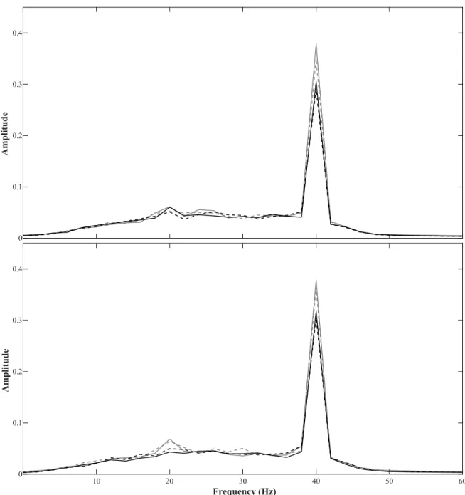
The continuous EEG recordings of the amplitude modulation test were processed following the same first seven steps as described for the Adaptation test (see above). The applied FIR filter in this test had a lower edge frequency of 1 Hz and a higher edge frequency of 40 Hz. Subsequently to step 7, the epoched signal was imported into Letswave 6, a matlab toolbox by André Mouraux, (http://nocions.github.io/letswave6), to perform the final processing steps. In Letswave (1) average ERPs were calculated for each participant and stimulus frequency. (2) Each average ERP was baseline corrected applying a Frequency spectrum signal to noise ratio (SNR) transform. (3) Fast Fourier Transform (FFT) analysis were performed to ascertain cortical responses to the 40 Hz amplitude modulation. (4) Mean FFT values were calculated for each stimulus, test session, and participant based on the maximum peak response between 38 Hz and 42 Hz across all channels (see Figure 2.3). In preparation for data analyses mean FFT values were z-score normalized for each participant across stimuli and test sessions.
-3 -2 -1 0 1 2 3 4 V) (μ de itu Ampl -1 50 -1 00 -5 0 0 50 10 0 15 0 20 0 25 0 T im e in m s -3 -2 -1 0 1 2 3 4 V) (μ de itu Ampl -1 50 -1 00 -5 0 0 50 10 0 15 0 20 0 25 0 T im e in m s A B D C F ig u re 2 .2 : A da p ta ti on t es t: G ra n d av er ag e E R P s. G ra nd a ve ra ge E R Ps f or e ac h pr ob e to ne p re se nt ed d ur in g th e A da pt at io n te st . G re y sh ad ed sq ua re s in di ca te r an ge o f th e N 1-P2 w in do w u se d to c al cu la te t he A U C v al ue s. S ha de d ar ea s in di ca te t he s ta nd ar d er ro r ac ro ss p ar tic ip an ts . P re -t es t re su lts a re s ho w n in l ig ht g re y, p os t-te st r es ul ts a re s ho w n in d ar k gr ey . A : R es po ns e fo r th e 25 0 H z to ne . B : R es po ns e fo r th e 35 4 H z to ne . C : R es po ns e fo r th e 70 7 H z to ne . D : R es po ns e fo r th e 10 00 H z to ne .
Figure 2.3: Amplitude modulation test: Mean FFT. Mean FFT values for test frequencies of the amplitude modulation test. Pre-test results are shown as dashed lines, post-test results are shown as solid lines. Upper plot: Test frequencies of below-notch range. In lighter grey responses for 250 Hz tone, in darker grey responses for 354 Hz tone. Lower plot: Test frequencies of within-notch range. In lighter grey responses for 707 Hz tone, in darker grey responses for 1000 Hz ton.
0 0.1 0.2 0.3 0.4 A m p li tu d e 10 20 30 40 50 60 Frequency (Hz) 0 0.1 0.2 0.3 0.4 A m p li tu d e
2.3. Analyses and Results
The effect of notched-music listening was ascertained by analyzing differences in cortical activations between pre-test and post-test recordings for test frequencies below and within the music notch (notch range activations), as well as for each test frequency separately (frequency activations). The same analyzes were applied to both EEG tests, adaptation test and amplitude modulation test. All results reported in this sections have been adjusted for multiple comparisons (i.e., Bonferroni correction).
2.3.1. Music listening
Analyzes of the daily music listening questionnaires revealed that participants have listened in average to 34 hours of notched music throughout the music listening period (range 22 to 47 hours), and in average 3.2 hours of notched music listening per day (range: 2.4 to 4 hours). Results of an independent t-test showed no differences in the reported hours of music listening between the two participant groups which have been created due the performed test order (t(14) = -.835, p = .418, r = .218), where r represents an effect size measure that is calculated, following Field (2009), as sqrt(t2/(df + t2)).
2.3.2. Adaptation test
2.3.2a. Notch range activations
Notch range activations represent the combined responses of test frequencies within one notch range. Each notch range activation is based on the difference between the frequencies of one notch range and has been calculated, for each notch range and test session,
by subtracting the 1-octave tone response from the related 0.5-octave tone response (below-notch: 250 Hz - 354 Hz; within-notch: 1000 Hz - 707 Hz). Subsequently the obtained post-test values were subtracted from the pre-test values to estimate changes in activation across test sessions and the resulting values have been used in the following analyzes. Upon inspection of the data, an outlier was detected for the within-notch measure with a mean value more than two standard deviations apart from the sample mean (see Figure 2.4). The data of this participant were excluded from all adaptation test analyses. The distribution of both notch ranges were tested for normality applying Shapiro-Wilk tests. Both distributions were found to be normally distributed (below-notch: W(15) = .965, p = .779;
within-notch: W(15) = .908,p = .124). The use of parametric tests in the following analyzes is therefore adequate. Subsequently, independent t-tests were performed to test the effect of test order, which revealed no significant difference between participants who performed the Adaptation test first or last for both distributions (below-notch: t(13) = 1.425, p = .178, r = .368;
within-notch: t(13) = 1.012, p = .330, r = .270). The variable Test order will therefore be ignored in the following analyzes.
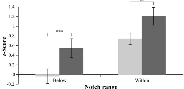
The changes in notch range activation across test sessions was analyzed for each notch range applying one-sample t-tests with the test value 0. Results show significant differences between pre- and post-test session for both notch ranges (below-notch: t(14) = -4.325, p < .001, r = .756, within-notch: t(14) = -3.023, p < .01, r = .628,). For both distributions, a significant increase in activation differences was found for post-test measures relative to pre-test measures, indicating a change in the processing of frequencies due to the notched-music listening period (see Figure 2.5).
Figure 2.4: Adaptation test: Participant data for within-notch range across test sessions. Participants mean activation for the within-notch range are shown as stars. Participant mean is shown as grey dashed line. The grey shaded area indicates the range of 2 standard deviations around the participant mean. The outlier, which is more than two standard deviations apart from the sample mean has been removed from all analyzes of the adaptation test.
Figure 2.5: Adaptation test: Notch range activations across test sessions. Notch range activations represent mean differences between frequencies within each notch range per test session. Pre-test values are shown in light grey, post-test values are shown in darker grey. Error bars indicate standard error across participants. Significance levels of performed analyzes (one-sample t-test: Notch range activation across test sessions) are indicated as follows: *** p < .001; ** p < .01; * p < .05. 1 2 3 4 5 6 7 8 9 10 11 12 13 14 15 16 -2.0 -1.0 0.0 1.0 2.0
Participants
A
ct
iv
at
io
n
(
μ
V
)
Below Within -0.2 0 0.2 0.4 0.6 0.8 1 1.2 1.4Notch range
** * * *z-S
co
re
2.3.2b Frequency activations
In a second set of analyses the effect of notched-music listening was ascertained for each of the presented frequencies. The difference between frequency responses across test sessions was calculated for each test frequency by subtracting its post-test activation from its pre-test activation. The resulting values have been used in the following analyzes. Shapiro-Wilk tests were applied to for violations of the normality assumption. Results indicate that all distributions are normally distributed (250Hz: W(15) = .928, p = .251; 354Hz: W(15) = .937, p = .351; 707Hz: W(15) = .944, p = .433; 1000Hz: W(15) = .964, p = .760). Independent t-tests were performed to test the effect of test order. Results reveal no significant differences between the two participant groups (250Hz: t(13) = 1.469, p = .166, r = .377;
354Hz: t(13) = .483, p = .637, r = .133; 707Hz: t(13) = .320, p = .754, r = .088;
1000Hz: t(13) = .905, p = .382, r = .243). The variable test order will therefore be ignored in the following analyzes. Differences between pre- and post-test activations were analyzed for each test frequency applying one-sample t-tests with the test value 0. Results indicate a significant difference between pre- and post-test activations for test frequencies 1 octave below and 1 octave above the edge frequency with a significant increase in activation for the post-test relative to the pre-test for both test frequencies (250Hz: t(14) = -2.899, p < .05, r = .612;
1000Hz: t(14) = -2.633, p < .05, r = .575). No significant difference between pre- and post-test activations were found for test frequencies 0.5 octave below or 0.5 octave above the edge frequency (354Hz: t(14) = .037, p = .971, r = .010, 707Hz: t(14) = -.900, p = .383, r = .234; see Figure 2.6).
Figure 2.6: Adaptation test: Frequency activations. Frequency responses across test sessions. Pre-test values are shown in light grey, post-test values are shown in darker grey. Frequencies left of the dotted line lie below the music notch, frequencies right of the dotted line lie within the music notch. Upper plot shows mean frequency responses before z-score transform. Lower plot shows z-normalized data (data used for analyzes). Error bars indicate standard error across participants. Significance levels of performed analyzes (one-sample t-test: Frequency activations across test sessions) are indicated as follows: *** p < .001; ** p < .01; * p < .05.
250 Hz 354 Hz 707 Hz 1000 Hz 0.0 0.5 1.0 1.5 2.0 2.5 3.0 3.5 Stimuli A ct iv at io n ( μ V ) 250 Hz 354 Hz 707 Hz 1000 Hz -1 -0.5 0 0.5 1 1.5 2 Stimuli z-Sc or e * *
2.3.3. Amplitude modulation test
Following the analyzes of the Adaptation test, the effect of notched-music listening was ascertained by analyzing differences between pre- and post-test session for both notch ranges activations, as well as for each test frequency.
2.3.3a. Notch range activations
The two notch range distributions were tested for normality applying Shapiro-Wilk tests, and both were found to be normally distributed (below-notch: W(16) = .976, p = .929;
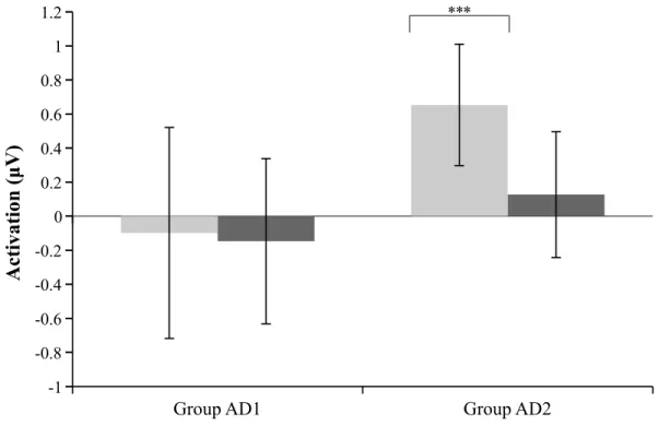
within-notch: W(16) = .941, p = .359). The effect of test order was analyzed via independent t-tests. Results reveal a significant effect of test order for the below-notch range (t(14) = -2.974, p < .01, r = .622), indicating differences in the measures of the below-notch range between participants who performed the amplitude modulation test first (AD2) or last (AD1). No effect for test order was found for the within-notch range differences (t(14) = -1.272, p = .224, r = .322). Due to the significant effect of test order, found for below-notch range measures, analyzes for this measure will be performed individually for each group. One-sample t-tests with the test value 0 were performed to analyze differences across test days for each notch range. The within-notch range difference was analyzed across all participants (N = 16). The below-notch range difference was analyzes with two separate t-tests, one for each group (n = 8). Results reveal a significant difference for the below-notch range for group AD2, with significant increased frequency differences in post-test measures relative to pre-test measures (t(7) = 5.182, p < .001, r = .891). No significant difference between pre- and post-test were