Analysis and design of multipole, super-conducting rotating electric machines for ship propulsion.

ANALYSIS AND DESIGN OF MULTIPOLE, SUPERCONDUCTING ROTATING ELECTRIC MACHINES FOR SHIP PROPULSION

by

Joseph Vito Minervini

B.S., United States Merchant Marine Academy (June, 1970)

Submitted in Partial Fulfillment of the Requirements for the Degree of Master of Science in Mechanical Engineering

at the

MASSACHUSETTS INSTITUTE OF TECHNOLOGY February, 1974

Signature of Author:

arfent-of Mechahical Engineering

January 23, 1974

Certified by:

Accepted by:

Thesis Apervisor

Chairman, Departmental Committee on Graduate Students

Archives

APR 11974

ANALYSIS AND DESIGN OF MULTIPOLE, SUPERCONDUCTING ROTATING ELECTRIC MACHINES FOR SHIP PROPULSION

by

Joseph Vito Minervini

Submitted to the Department fo Mechanical Engineering on January 23, 1974, in partial fulfillment of the requirements for the degree of Master of Science in Mechanical Engineering.

ABSTRACT

The use of superconducting electric machines for ship propulsion offers several advantages in increased power den-sity, flexibility of plant layout, and elimination of large reduction gears and propeller shafts.

In this study large diameter, multipole synchronous machines are modeled as linear machines with flat armature and field windings. Full field, inductance, and power rating expressions are developed for a linear geometry and compared with corresponding cylindrical expressions.

A 29.82 M.W., 60 pole, 120 R.P.M. motor is designed from this model and compared with a conventional synchronous motor designed for a ship propulsion system. An analysis of motor starting and synchronizing is also included.

Thesis Supervisors Philip Thullen

3

ACKNOWLEDGMENT

I would like to acknowledge the guidance of my advisor, Professor Philip Thullen, who molded my erratic efforts into

a somewhat distinct path. Particular thanks go to Doctor Thomas Keim who led me through some rather sticky places, in

TABLE OF CONTENTS PAGE Abstract 2 Acknowledgment 3 List of Figures 5 List of Tables 6 Glossary of Terms 7 I. Introduction 11

II. Linear Analogy of Large, Multipole 14 Synchronous Machines

III. Design of a Motor 33

IV. Motor Starting 46

V. Conclusions 63

Appendix A. Field Analysis of Linear Geometry 65 Appendix B. Limiting Analysis of Cylindrical 73

Expressions

Appendix C. Alternative Design 76

LIST OF FIGURES PAGE 1. Field and Armature Configuration ₁₅ 2. Field Intensity Variation in Y- Direction 20

3. Field Intensity Variation in X-Direction 21

4. Angular Orientation of Field 22

5. Voltage-Current Relationship 25

6. Armature Thickness Effectiveness 28

7. Power Density versus Pole Pitch 30 8. Power Rating Ratio versus Pole Pairs 34

9. Comparative Motor Sizes, Side View 39

10. Comparative Motor Sizes, End View 40

11. Magnetic Shear Stress versus Machine Rating 44

12. Configuration for Solution of Fields 48 Around Damper Shield

13. Contour for Calculation of E Field 48 14. Field Attenuation versus Slip Factor 56

15. Induction Starting Forces on Damper Shield 59 16. Current Distribution in Current Sheet 66 17. Configuration for Solution of Magnetic Fields 68 18. Configuration of Full Field Winding 70

LIST OF TABLES PAGE

I. Glossary of Terms 7

II. Field Expressions for Linear Winding Geometry 16 A. Full Expressions

B. Without Lower Iron Shield C. With Nb Iron Shields

III. Self and Mutual Inductance Expressions 23 for Linear Winding Geometry

IV. Electrical and Mechanical Machine Parameters 38 V. Comparison of Magnetic Shear Stress Levels for 42

Various Superconducting and Conventional Electric Machines

VI. Constants for Field Expressions Around 52 Damper Shield

VII. Simplified Field Expressions Around 54

TABLE I Glossary of Terms Symbols A b Bsat D Ef E g Ia If Ja Jf k K L La Ld L f Lab Lad Ma M N Nat Nft n p p

Cross-sectional area of one pole winding Pole face dimension

Magnetic flux density

Shield material saturation flux density Outside diameter of rotor

RMS open circuit voltage Electric field intensity Magnetic force density Air gap dimension

Magnetic field intensity Rated RMS armature current Rated field current

Rated armature current density Rated field current density Wave number, Chapter IV Sheet current density Pole pitch

Straight section length

Armature phase-a self-inductance Damper shield self-inductance Field winding self-inductance

Mutual inductance, phase-a to phase-b Mutual inductance, phase-a to damper Mutual inductance field to phase a

Vertical distance from origin to upper iron shield Vertical distance from origin to lower iron shield Number of armature winding turns

Number of field winding turns

Positive integers (1,2,3,...) indicating harmonics Number of pole pairs

TABLE I (cont'd) r R Rm Rt s S Swf Swa t a tf td t s u Vtip Vt xa Xa X Y Radius

Winding or shield radii, subscripted Mean radius of field winding

Damper shield radius Slip

Slip factor used in damper shield analysis Field winding dimension

Armature phase winding dimension Armature winding thickness

Field winding thickness Damper shield thickness Magnetic shield thickness

Horizontal coordinate in fixed frame, Figure Tip velocity of rotor

Rated terminal voltage

Synchronous reactance, per unit with Ef as base voltage

Synchronous reactance, ohms Rai/Rao

Rfi/Rfo

Distance from x axis to outside of field windin Distance between damper current sheet and armat current sheet

Distance from x axis to inside of armature wind Distance between damper current and iron shield

2A (Appendix C) fo

Distance from x axis to inside of iron shield Skin depth

Rotor axis displacement from phase a axis, (Figure ) cartesian coordinates

g

ure ing

TABLE I (cont'd) Angular displacement

Field winding included angle

PEwf

Armature winding included angle pewa

wa

Subscripted, flux linkage nYJ

n, Appendix A

Magnetic permeability Conductivity (mhos/meter) Surface conductivity (mhos)

Rotor axis displacement from phase-a axis, cylindrical coordinates

Scalar potential, Appendix A Power factor angle

Angular velocity or frequency Subscripts a a b c d f i m o s w w Armature winding Phase a Phase b Phase c Damper Field winding Inner, inside Mutual Outer, outside Shield Winding Within wfe 0 wa 0 wae 1' S

10

TABLE I (cont'd) Superscripts

a Damper shield analysis, region between iron shield and armature current sheet

b Damper shield analysis, region between armature current sheet and damper current sheet

c Damper shield analysis, region below damper current sheet

Chapter I. Introduction

The application of superconductors to rotating electric machinery promises advantages over conventional electric machine technology. This is especially true in the use of superconducting electric generators and motors for marine propulsion systems.

In general, superconducting electric propulsion plants with gas turbine prime movers offer many advantages over steam turbine systems and diesel engines in weight and volume reduction of the overall system. Also, the elimi-nation of large, direct mechanical reduction gears and long propulsion shafts results in a highly desirable flexibility of component placement. Gas turbine-generator set units can be placed in positions readily accessible for easy

main-tenance, and intake and exhaust ducting lengths may be considerably decreased. Motors can be directly coupled to the propeller shafts. For certain high performance craft, entire steerable pods containing motor and propeller may be practical. In large propulsion systems the parallel

oper-ation of several generators and motors offers a wide range of operating modes for different load, speed, and emergency conditions.

The technical and economic reasons for considering superconducting electric propulsion systems are many. However, there are some important problems that must be

overcome. Ship drive systems must be capable of operating at several different maneuvering speeds between zero and normal cruising speed. In electric systems this can be accomplished by several different methods. One of these is by varying the electrical frequency of the motor by means of a frequency or cycloconvertor. Another method is to have the motor-generator speed ratio fixed by the field-pole ratio of the two machines in a synchronous system and then affect propeller speed changes by varying the prime mover speed. This results in inefficient operation of the prime mover during maneuvering operations involving many speed

changes. However, for normal commercial vessels, the time spent maneuvering is only a small fraction of the time spent at normal cruising speeds where the system is designed for

optimum efficiency.

This work is concerned with solving the problems en-countered in the design of a large power rating, slow speed, multipole, synchronous electric motor for use with a

synchronous generator. In this type of system a large speed reduction is necessary for the efficient operation of a high speed prime mover, such as a gas turbine, coupled with the relatively slow speed propeller. This requires a large number of field poles on the motor. For large power requirements, the problem, then, is to get enough of the flux created in the field windings to link the armature

windings. Electric machines with large air gap to pole pitch ratios have a large amount of leakage flux if not properly designed. Conventional machines have iron in the rotor core and stator flux circuits to enhance flux linkage with the armature windings and reduce leakage flux. Iron is not used in superconducting machines because the high magnetic fields created would exceed the saturation limit.

Early efforts in this study to solve this problem centered on non-conventional geometries to improve flux linkage, and these may be found in Appendix C. However, this approach did not yield very encouraging results. Therefore, the principal approach taken was to model a large diameter, multipole, cylindrical machine as a flat stationary armature and a flat, moving field winding. This proved to be a good simplified model. The field expressions developed from this model can be reduced to a very simpli-fied form which is easy to use and understand. The effects of changing certain design parameters are readily computed. This yields a relatively easy method for the first rough design of large, multipole synchronous electric machines.

The next step taken was the design of a superconducting motor based on these results and a comparison of this design with a conventional ship propulsion motor proposed by one

of the major electric machinery manufacturers. This is primarily an electrical design with minimum consideration given to the mechanical and thermal design.

Chapter II. Linear Analogy of Large, Multipole, Synchronous Machines.

A linear (flat) stationary armature and moving linear field winding were used to model the stationary armature and rotating field winding of a large diameter, multipole, cylindrical synchronous electric machine. Field expressions were derived for a flat, three phase, armature winding and flat field winding with ferromagnetic upper and lower

shields. Figure 1 shows the physical configuration. The derivations are presented in Appendix A and the results are summarized in Table II.

This is a two-dimensional analysis. The field ex-pressions were done on a per-unit length basis, and actual end-turn effects were not analyzed.

The actual physical arrangement of a superconducting machine can be modeled mathematically by setting the lower iron shield at an infinite distance from the field winding. This leaves the moving field winding, stationary armature and the upper iron shield as the components of the machine. Except for the upper iron shield, there is no ferromagnetic material in the machine. These expressions may be simplified

even further by placing the upper iron shield at infinity. The form of the field expressions demonstrates explicitly the field variations in the x and y directions.

AXIS OF FIELD WINDING I AXIS _{OF PHASE A}

A+

C-

B

A-

C+

B-

A+

I

_I

-

_I

B+

A-

C+

B-V

I

.-s

I

I

TABLE II

FIELD EXPRESSIONS FOR LINEAR WINDING GEOMETRY

N < y < -t /2 - f H = xfi n odd 4Jf _{n Swf} - sin( ) 2 2 2% nT -2nTrM (1+e - ) n7T t -2nvM -2nwN 2R (e A - e T ) -nery n )-[e - (y-2N) H y = -yfi n odd -2nrM nt 4

f sin ) (+e sinh ) X

2 2 2R -2nTM -2nN 2 n (eT- e A ) (-2N) -ngyr [e- y - 2 N ) + e k ] -t f/2 < y < +t f/2 Hxfw = n odd xfw n odd 4J f f 22 n r nir S wf sin( 2 -2n7rM -2nrN (e - e , ) nht -n- nN fsinh \ 2kf - e (y-2M-2N) + -ns sinh(-n [e-(t /2+2N) s n r) 4J f yfw n odd 2 2 nir n(tf/22]} os e -(t /2-2M)]} Cos(nrx f ]~ ck nSTwf sin( (-2 ) -2nrM -2nrN -2nrM -2nrN (e e + (e T-e eT ) t t -nu f n tf nvt nu -n n

cosh( ) [e-- 2N e -2M)]-sinh( f (e-(y-2M-2Ne a ]}sin( )

k k, nox cos (--) k nux sin 9,T~

+tf/2 < y < M -2nvN 4J Z n7TS H 4J f n wf (1+e k ) xfo n odd 2 2s 2 -2n M -2nvN [e k -e k ] nTft sinh( ) 2k - n _{eX - e --}jy n -r_(y-2M) [eA - eA] H = -E yfo n odd 4Jf 9, f 2 2 n T .n Swf sin( - ) 2R -2nrN (l+eT -') -2niM -2nTN [e - eT ] nt sinh( --- ) 29 nI(2M -n7T [e ( y - 2 M)+ e 9 ] TABLE IIB

FIELD EXPRESSIONS WITHOUT LOWER SHIELD

(lim N -* -co) y < -t /2 f H E 4JfZ xfi n odd 2 2 nT[ H yfi odd yfi n odd nT Swf sin( 29 ) 2 A 4 Jf nS wf 2 2 sin( 2, ) 2 2 2 n Tr ntf sinh (- n-) finh sinh( ) 2R -2nM nry [(l+e )e ] cos ( ) -2nTM nry [(1+e 9 )e , ] sin(-- ) k -t f/2 < y < +tf/2 xfw = 4J f n odd 2 2 nTr H yfw odd yfw n odd nTrS ny t n 2M -nT tf sin( - )[sinh(--- )e--( y - _2M)-sinh(n

)e- -] cos( )

4Jf, nTS nTt nTr -nTt f

f wf f (y-2M) f (nTy

2 in( )[+sinh(-- )e (y-2M)-cosh(n T)e ] sin(nx

nT cos(nx) - -nwx sin ( -) k,

18

+t f/2 < y < M

4J f nSwf n7T t nTr -,ny T

H E sin(f ) sinh(T- - e ] cos(nrx

xfo n odd 2 2 2 P 2

nw

4J f n7TS nTrt n 27T -n7T

Hyfo od sin( ) sinh( ) [e - ( y - M+ e x sin(x

H

yfo n odd 2 2 2Y n 2s

TABLE IIC

FIELD EXPRESSIONS WITH NO IRON SHIELDS

(lim M - oo) (lim N -* -)

y <_-t /2

4Jwf nS nTt n7 Hxf odd 22 sin( ) sinh(--) e cos

xfi n odd 2 2 2R 2R R

n 7

4Jf n Swf n t n s )

H 4 sin( ) sinh( n t) e T sin( )

yfi n odd 2 2 sin( sinh( 2 nu

-tf/2 <_ y < +tf/2

-nft

4Jft n wf i . y ,x

H -sin( n= ) sinh ) e 2Y cos(--)

xfw n odd -2 2 2

H = sin( ) [1 - cosh(ny e ] sin(-)

y < +t /2 f 4J f H =

e

cos

IHI

SIN(3

= .3 053

o.s50

FIRST HARMONIC TERM

0.40

,3

2

=0

FIG. 2

FIELD

INTENSITY VARIATION

2 2 4 4 2 2 2

74 J

A= .3053 0.50-YUQ ya.

y.

tj/

II

0.40-1-+

INTENSITY

VARIATION

IN

I

,~B s,.RI

)

IV

X

_

V

.Y= 0

Y-6=

ARC TA

NTAN (

ToANAIs)1

-SIN H - ) I I I _I X

8

4

8

2

8

FIG.

4

ANGULAR

8o

oQ

ORIENTATION

OF

FIELD

TABLE III

SELF AND MUTUAL INDUCTANCE EXPRESSIONS FOR LINEAR WINDING GEOMETRY

N' =N+ (g Maf = -odd pL n odd t t + +) 2 2 16p , 55 n 7 N nTS ft wf ( )sin( ) wf f N at S ta wa a t t M' = M- (g +t +2 ) 2 wa nwd sin( S) cos( -) x 21 k -2nrN (1+e k ) -2nirM -2nirN (eT F- eZ' T ) nrt -2n:M nTy nlTw -nw -n7 sinh(- ) [e F (e - e )+(e - )] 2 Lf pL n odd 32po k 55 niT Nft 2 2 nSwf nt ( sin ( ){ f St 2f 2 wf f tf ntf [e-( + N)-2 +sin( -2n2 2R -2n'fM en~ (-2M)] -2nrN (e -- e 7-) -nr 2 nhtf [1+e -(2M + 2N) - sinh ( [l+e 2 -2n M -2nN (e 2 - e ) 32p 04 n odd 5 5 n T Nat 2 2 wa ta N ) sin ( w){ S t _{2 2} wa a t t -nT a nT a v nh ta [ e-- +2N')- _e (-2M 2/ -2nrM -2nvN (e I-- e ) n2 nT a [1+e-g ( 2 M ' + 2 N ' ) - sinh2( a r 1 2k -2nwM' -2nrN' (e T - e- ) L Lab pL n odd 32p1Y4 55 nT Nta ₂ wa a n2 ( wa 2n sin ( ) cos( 2R 3 t nta te-n-~ +2N') sinh (a) I e---2nMN

en- ( -2M')

-2nirN'

n2 a

-sinh2 2.

(e - - e e )

(All inductances are for one pole pair)

(1+e (2M'+2N') -2nrM' -2nirN' (e 2 - e ) L a pL flirt a (2_2R

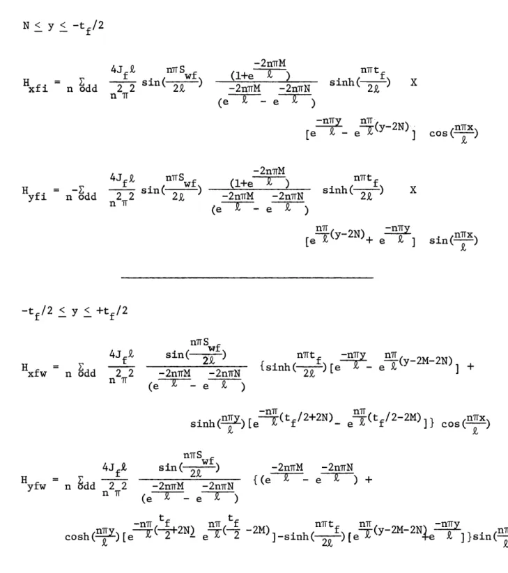
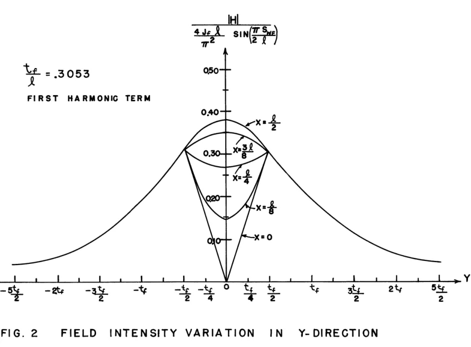
Figures 2 and 3 show graphically how field intensity, H, varies in these directions. The variation of the field

in-tensity in the y direction is shown in Figure 2. Figure 3 demonstrates the field variation in the x direction. The angular orientation of the field is displayed in Figure 4.

Expressions for the self and mutual inductances of the field and armature windings are derived by integrating the fields over the area of the windings. This is done in Appendix A and presented in Table IL These expressions are also based on a per-unit straight section length.

The field intensity expressions contain terms for armature current density and field current density. These are given by:

Nft If Nat Ia

f Swf t and a Swa ta

where Ia is the r.m.s. value of armature terminal current. Power Rating

With these expressions we can now derive a power rating for the linear geometry machine.

Vt P = 3VtIt = 3EfIt(E-)

V_t is rated terminal voltage, It is related to current density by the armature winding geometry and Ef is gener-ated internal voltage, given by:

E= eMlIf = Vtip

FIG.

5

VOLTAGE

CURRENT

RELATIONSHIP

XAlA

Ef is the r.m.s. value and Vtip is the velocity of the

moving field winding. Power then is:

-2'iM 1 48 w 'P J J L 9 kwa S f l+exp( ) P - o5 sin )sin(eofa tf where y = _g+ -+ t_a rttf -27 rM T X sinh(f e (e ) + (e -e

- e

(f-)

+--As there is no iron within the field winding of a super-conducting machine, we can simplify this by removing the lower iron shield.

lim N

--48 4 T wf awa tf)

P - eo J J aL sin(-2T-) sin( 2 ) sinh(2R X

-r2 r f( Z- 2 2 -27 M ,

e T(e

vt

and (E ) =1 - Xa cos - Xasin f

(See Figure 5 )

Cos i is the power factor and Xa is per-unit synchronous reactance with Ef as base voltage.

Xal a x =Ef

e (La _{- Lab)Ia}

_

a _Ef

4~(La _{- Lab )Ia} M If

Figure 5 shows the voltage-current relationship.

For first harmonic terms only, and no iron shields (lim N -- - , M M -- + W), this expression becomes:

utwa ta _7rta La Ja sin 2a a - eg/

a L m _mf Jf sin( wf _{2 ) l-e --} - al _l-e-7f

This expression, along with the simplified power rating

expression (lim __ _ utf _ Tt_a

w-

-

-

a

p 24 Z 4 PL J J sin( wf) sin(TS wa (-e )(-e )

- 'Tg V X (e ) ( -)

f

First we can see that the power falls off exponentially with the characteristic air gap dimension, E . It becomes

obvious that we should design a machine with the minimum air gap necessary for mechanical clearance.

The term that contains the armature geometry effects, - Ita

(1-e k ), indicates that there is a point of diminishing effectiveness for increases of armature thickness, as shown in Figure 6. Pm is the power output from a machine with an armature of infinite thickness. An armature thickness can be chosen for the initial design that gives, perhaps, a 90%

or 95% effectiveness.

Although the power rating expression has a similar term for the field winding thickness, (1-e Z ), the same criterion of effectiveness cannot be used to determine an optimum field

P/P.O

winding dimension. This dimension must be determined by taking into account the maximum field density which occurs within the winding volume.

A superconductor may be driven into the normal region by an excessively strong magnetic field. Therefore, the magnetic characteristics of the superconductor must be

known to choose the maximum value of flux density, with

sufficient operating margin from the transition line between normal and superconducting regions. The field winding

thickness required to achieve this operating point can then be calculated from the field intensity expression for the region within the winding volume.

Power Density

The linear dependence of power rating (or power density) with field current density demonstrates a major advantage of superconducting machines over conventional machines. This is because superconductivity allows the use of much higher field current densities than are possible in conventional machines. Figure 7 demonstrates this point. Power density is the power per active volume of one pole pair.

P

Lm2k (tf+g+ta) = Power Density

For this particular study certain parameters were fixed. ar Swf

The winding dimension, -2 -- , was chosen so as to make

300

250

N200

I

150

(METERS)

thickness that gave a ninety percent effectiveness was chosen, i.e. (t_a = .735 a). For simplicity, the air gap dimension was assumed to be zero. The characteristic field winding

'it

thickness, ---- , that gave a maximum field density of 40 kilogauss, was used. This ratio of field thickness to pole pitch varied with different values of k, but for the large pole pitches it is small compared with the armature thickness

ta

to pole pitch ratio (--). The power density could then be approximated by:

Power Density

22 Lm

Other parameters held constant were the electrical frequency,

We = 377 radians/sec, and the current densities,

Ja = 2.5 X 06 Amps/m2 and Jf 1.25 X 10 Amps/m2

Also, no iron shields were used. A family of curves could be plotted by varying any one of these parameters indepen-dently of the others. The curve for a conventional machine would have a similar shape but a much smaller slope due to the lower values of field current density that may be used.

The curve is nonlinear at the smaller values of pole pitch because the field thickness to pole pitch ratio is not negligible here. The power density goes to zero at some finite value of pole pitch because the synchronous reactance approaches unity at this value of pole pitch. This is really an artificial situation because Xa can be changed by

a new curve. The approximations and assumptions break down in this lower region, but good approximations of power

density can be made from the larger pole pitches in the linear region.

This curve may be used to determine several different parameters of the machine. There are several expressions relating machine parameters which may be used in the approx-imation of a large cylindrical machine.

TV

£ _ tip _TR

V _{= WR}

W p tip m

e

With these relations and the pole pitch versus power density curve (Figure 7) we can determine the machine dimensions. Usually the electrical frequency, we , at which the machine will be operated is known. Also, the mechanical speed is known from the speed requirements of the load. These two

frequencies then will determine the number of the poles

required on the motor. If a tip speed is known, this, along with the mechanical speed, will fix the rotor diameter and the pole pitch.

We have thus far determined the electrical frequency, rotor speed, tip speed, rotor diameter, number of poles, and the pole pitch. A power density of the machine can then be determined from Figure 7 for the corresponding pole pitch. Thus, an approximate power rating per unit length is deter-mined. This linear analysis demonstrates the ease of deciding machine parameters for a first approximation.

Chapter III. Design of a Motor

With the linear geometry model complete, the next step is the design of a large power rating, multipole, synchronous motor based on this new model. First, however, the validity of the model must be determined. The accuracy of the linear expressions for the field intensities and the inductances was checked by taking the limit of the corresponding

cylindrical geometry expressions as the number of pole pairs and the radius approach infinity. By careful use of power series expansions it can be shown that;

Lim L(r,e) = L(x,y) Lim H(r,O ) = H(x,y)

R -+ 0 R

-This limit-taking process is done in Appendix B.

Once the accuracy of the expressions has been checked, it must be shown that they are good approximations of the cylindrical expressions for multipole machine designs. This can be done by comparing the power rating expressions over a range of pole pairs. The results of this analysis are shown in Figure 8 where the ratio of the flat power rating to the cylindrical power rating is plotted versus pole pairs.

To actually compare the two expressions numerically, certain parameters were fixed. A family of such curves can be plotted by changing one of the independent parameters. For this study the speed was chosen as 75 feet per second

_ - . -- - -__- =--- - - - _{x R;D 83.6u} ll XRl 3 5 .8 " -/ / INCREASING 9. I R = 11.9 " S11. _VTI P= 75 F PS / f. =.1905 M

-I

t =:.05816 M

P(POLE

P

AIRS)

FIG. 8

POWER

RATING RATIO

VERSUS

POLE PAIRS

which is to be on the linear portion of the power density vs. pole pitch curve, Figure 7. The electrical frequency was fixed at 60 hertz. These two parameters, then, fixed the pole pitch,

k, at .1905 meters (7.5 inches). To maintain a constant pole pitch, the diameters of the machine had to vary directly

proportional to the number of pole pairs. In Figure 8, as we move to a higher number of pole pairs, we get increasingly

larger diameter machines.

R= EL where R (Rfi + tf/2) = (R tf/ 2 )

m Tr m fi f fo

The armature thickness, t_{a ,} was chosen from Figure 6 to yield a ninety percent effective armature. The field winding

thickness, tf, gives a maximum field flux density of

1.25 X 10 A/m2 . The air gap dimension, g, was arbitrarily chosen as one inch. Effects due to iron shields were

neglected, and Vt/Ef was held constant at unity.

The results of this analysis were consistent with the re-sults of the limiting case of the cylindrical expressions. The linear analogy yields poor results for small diameter machines with a low number of pole pairs, but rises asymptotically to unity as the pole pair number and machine diameter approach

infinity. This plot indicates that simplified linear power rating expressions give results of ninety percent accuracy for machines with fourteen pole pairs, a pole pitch of 7.5" and a radius of 33.4". The conclusion is drawn that a linear anaysis

yields a good approximation of large diameter, multipole, cylindrical machines.

Motor Design

The linear analysis is now used to design a large,

superconducting, propulsion motor. The motor is required to match the performance of a conventional synchronous motor proposed by the General Electric Co. for an electric ship propulsion system with gas turbine prime movers and speed control by varying prime mover speed. Comparisons of the two designs can then be made.

The motor is required to have a power rating of 40,000 horsepower (29.82 MW) at a shaft speed of 120 revolutions per minute. Gas turbine design speed is 3600 revolutions per minute. The direct coupled synchronous generator is a two pole, 60 hertz machine. This requires 60 poles on the motor for sychronous speed reduction to 120 r.p.m. The

three steps of the design procedure are: 1) determine primary machine dimensions from the linear expressions

for the initial design; 2) utilize the dimensions determined in step one in the cylindrical expressions for the actual machine design; and 3) compare the superconducting machine design with the conventional design. Table IV lists the machine parameters determined from step one and step two. In the linear analysis the tip speed of seventy-five feet per second was chosen from the linear portion of Figure 7.

The tip speed, along with the electrical frequency, determine the pole pitch. The pole pitch and the pole pair number

determine a mean radius (Rm). m rr

The superconducting machine in this design has a maximum field of 40 kilogauss in the winding with a field current density of 1.25 X 108 A/m2 . This requires the field winding to be 2.29 inches thick. An air gap dimension of one inch was chosen to allow for mechanical support structure and an electro-thermal damper shield. A magnetic iron shield was positioned just behind the armature winding. The minimum thickness required is determined from Bmax < Bsaturation

within the magnetic shield. Saturation of iron occurs at a flux density of about 15 kilogauss. An armature current density of 2.5 X 106 Amp/m2 is assumed. All of these para-meters can be then used in the power rating expression to determine the straight section length required to produce

29.82 megawatts.

With these parameters determined, the equivalent dimen-sions were substituted into the cylindrical power rating expression. A new machine length, shorter than the flat

rating length, was calculated. Results are listed in Table IV Step three of this procedure entails a comparison of

this new superconducting motor design with a conventional motor design for similar performance requirements.

TABLE IV

Electrical and Mechanical Machine Parameters

Power Rating: P Shaft Speed: N

Electrical Frequency: we

Power Factor: cos

P

Number of Poles: 2p Rotor Tip Speed: Vti_p Pole Pitch:k

Field Winding Thickness: tf Armature Winding Thickness: ta Air Gap Dimension: g

Inside Field Radius: Rfi Outside Field Radius: Rfo Inside Armature Radius: Rai Outside Armature Radius: Rao Magnetic Shield Radius: R_s Magnetic Shield Thickness: _{t s} Armature Radius Ratio: X Field Radius Ratio: Y

Maximum Field in Winding: _Bmax Effective Length: _Lm

Synchronous Reactance: _xa (Normalized to Ef)

Armature Current Density: Ja Field Current Density: Jf

Linear 40,000 HP (29.82MW') 120 R.P.M. 60 Hertz 1.0 60 75 fps 7.5 inches 2.29 inches 5.56 inches 1.0 inch 1.35 inch 40 kilogauss .52855m 20.blin. .169 2.5x106 Amp/m2 1.25x10 Amp/m2 Cylindrical 40,000 HP (29.82 MW) 120 R.P.M. 60 Hertz 1.0 60 75 fps 7.5 inches 2.29 inches 5.56 inches 1.0 inch 69.23 inches 71.52 inches 72.52 inches 78.08 inches 78.05 inches 1.35 inch .9293 .9650 .27 2.5x106Amp/m2 1.25x10 8Amp/m2

FIG. 9

COMPARATIVE

SIDE VIEW

CONVENTIONAL IRON

MOTOR

SIZES

FIG. 10 COMPARATIVE

END VIEW

CONVENTIONAL

IRON

MOTOR

SIZES

The General Electric Company has a design for a

40,000 HP, 60 pole, 120 R.P.M. synchronous motor for a ship propulsion system. Exact electrical and mechanical para-meters are not available, but overall physical size can be compared with the superconducting design. The conventional motor has an overall outside diameter of twenty-six (26) feet compared with fifteen (15) feet for the superconducting design. The rotor lengths are of about equal dimensions; approximately four (4) feet. Figures 9 and 10 demonstrate the approximate physical sizes and the significant increase in power density that can be obtained with superconducting machinery.

Another conventional propulsion motor design by the General Electric Company has approximately the same physical dimensions as this superconducting design. It is a 72 pole,

100 R.P.M., unity power factor, synchronous motor, but has a power rating of only 12,500 horsepower.

The comparison of the superconducting motor dimensions from this design with the large propulsion motors of the General Electric Company demonstrates explicitly the advan-tage of superconducting machinery in power density increases. By this analysis, a size reduction of approximately one-half

is possible by use of superconductors.

A simple method of comparing all rotating electric machines of varying dimensions, speed, and power ratings,

TABLE V

Comparison of Magnetic Shear Stress Levels for Various Superconducting and Conventional Electric Machines

Machine Power Mechanical Rotor Rotor (PSI)

Description Rating Frequency Diameter Length m

P(KW) OM D(in.) L(in) 1) AVCO, S.C. 8 1257 2.18 4.49 1.68 operating 2) First MIT 80 377 5.75 4.5 7.76 S.C. oper. 3) USSR S.C. 62 314 5.51 9.84 3.72 operating 4) USSR S.C. 1Xl03 157 20.3 21.4 4.07 operating 5) Second MIT 2X103 377 8.0 24.0 19.47 S.C. oper. 6) Westinghouse 5X103 377 10.2 17.6 40.81 S.C. oper. 6') Proj. capa- 1.5X10 377 10.2 17.6 147 bility Wvmod. 7) Westinghouse 3X104 18.85 87.25 27.0 43.4 S.C. Ship Drive Design 8) MIT Design 3X104 12.57 143.04 20.0 31.0 of Thesis 9) IRD, S.C. 5X 105 377 41.3 145.0 36.29 Paper design 10) MIT, S.C. 1X106 377 35.2 123.3 97.7 Paper design 11) G.E., S.C. 2 X106 377 43.0 117.5 98 Paper design 12) MIT, S.C. 1X106 377 21.6 130.0 246.4 IEEE Paper design 13) G.E. Ship 3X104 12.57 240 48 4.86 Drive Motor Conventional 14) Westinghouse 5X103 _{1257 10} 10.5 20.38 Airborne S.C. Operational

Machine Description Power Rating P(KW) TABLE V (Continued) Mechanical Frequency m Rotor Diameter D(in.)

15)Various conventional alternators, operating, mostly on (1964) 3 x 105 (1953) 4.4 X 104 (1953) 1.12 105 (1953) 1.47 x 105 (1953) 1.25x105 (1970) 8.0 x 105 (1970) 8.0 X 105 1.3o0 x lO5 AEP system: 377

377

377

377

377

38.0

56.0

15o.o

I0O

cn

0 0

W

0

I

(n

08

Z

It is a measure of the machine size and the average magnetic power transmitted across the air gap. It can be calculated from the power rating and the machine dimensions.

P _{= T"}

T = (shear stress)(surface area)(adius) = (m)(7TDL)()

2P

m _{r D2Lw}

m

This gives a quite simple measure of power per unit volume. A survey of various conventional and superconducting electric machines has been made, including both machines already in

operation and proposed paper designs. These results are listed in Table V and the corresponding values of magnetic shear stress versus machine rating are plotted on a log-log scale in Figure 11. This figure exhibits basically an

exponential growth in achievable shear stress levels with increases in magnetic shear stress of up to approximately an order of magnitude by superconducting machines over conventional designs.

Chapter IV: Motor Starting

An important requirement in the design of a synchronous motor is that it possess the ability to start itself by

induction motor action. This can be accomplished with short-circuited damper or amortisseur bars imbedded in the field pole faces to form a squirrel cage rotor. A cylindrical copper damper shield also serves the same purpose. With the unexcited field winding circuit closed through a large

resistance the motor should approach synchronous speed by induction motor action. Then when the external resistance is removed from the field winding circuit, and the field is excited, the rotor should pull into synchronism with the armature field.

In a synchronous system for ship propulsion this is difficult because the motor must be started under load, directly coupled to the propeller. During maneuvering operations the motor must be capable of being repeatedly

brought up to about one quarter of full speed ahead or astern and then synchronized, without excessive rotor heating. It would not be feasible to bring the speed of the motor up

from zero with the field energized by raising the gas turbine speed, because the turbine has a minimum idling speed.

This motor design utilizes a cylindrical conducting copper shield for induction motor starting and for use as an electrical damper winding during machine transients and

faults. An analysis of this damper shield was done to

determine its induction starting capabilities and its ability to be pulled into step. The analysis consists of three parts. The first step involves the solution of the fields created by the armature winding and the induced asynchronous currents

in the damper shield during starting. These fields are then utilized in part two to solve for the magnetic forces on the shield by application of Maxwell's stress tensor. These forces can then be converted into a torque-speed character-istic curve to analyze the motor's induction starting

capability. The third part of the analysis is to determine whether or not the rotor will pull into synchronism when the field is energized.

Solution of the Magnetic Fields

The damper shield can be modelled as a flat sheet with surface conductivity as permeability o and moving with velocity V. The armature is modelled as a flat traveling wave of surface current K;

K = K cos(w t - kx)T

where ws is the synchronous frequency of the armature

currents and k is the wave number. There is no contribution to the magnetic fields from the field winding because it is unenergized and short circuited through a large external

resistance during starting. Figure 12 shows the geometric configuration of the flat model.

2

//

HE

/)

TRAVELING WAVE V

I V

4

Xr-*

-CONDUC TING SHEET

2 I

L

3

FIG.12

CONFIGURATION

FOR

SOLUTION OF

FIELDS

AROUND DAMPER SHIELD

FIG. 13 CONTOUR FOR CALCULATION OF

E FIELD

We must solve for the B fields in the three regions a) between the armature and the upper iron boundary;

b) between the armature and the shield; and c) below the shield. One other unknown is Kf, the induced current in the moving shield conducting sheet. Maxwell's equations give us governing equations which apply in the three current-free regions, a, b, and c.

VXH = o and V.B = o

We know one other constitutive relation from the application of Ohm's Law in the moving current sheet:

K = E'

f s

Primes denote quantities measured in the moving frame. With the field transformations this becomes:

K = s(E + VxB) K' = Kf

E' = (E + VxB)

Now we can write H as the gradient of a scalar potential 0. H = -V

Therefore, Laplace's equation applies in the three regions. V 2 = 0

We can assume variable separable solutions of the form, P = X(x)Y(y)T(t).

In this analysis we assume there are no variations in the Z direction. We also assume the time varying part of the solution has the same form as the time part of the driving function.

T(t) = A cos w t + B sin t

By substitution into Laplace's equation, the form of the solution for H then becomes:

x = k {(cl ek+c 2e-ky)cos st sinkx- (ceky+c e-ky)sin

t _coskx

+ (c5eky+c6e-ky)sin Ust sinkx- (c7ek+ce-ky)cos wst cos kx} ix

H = k {(cleky-c2e - k y )c o s w st sin kx - (ceky+c e-ky)sin t cos kx

+ ky -ky (ceky -ky

+ (c7ek -c 6e-k)sin _{s t} cos kx + (c7ekc ₈e -k)cos _{s t} sin kx } y The boundary conditions that must be satisfied are:

1) at y = Ha =0 x 2) at y = a x(a b nx(H-H ) K -a -b x x = -K 3) aty= a S a b H a -H b y y 4) at y = 0 x (b

-c

One other equation is necessary to complete the solution. When applying Ohm's law on the moving current sheet we must carefully apply the integral form of Maxwell's equation to determine the E field on the sheet.

Choose a contour c in the fixed reference frame with the current sheet moving through the contour.(see Figure 13). The contour bounds an area length L in the z direction and differential widthdx) in the x direction. Assume components of the E field in the z direction only as we assume that currents only flow axially (z direction) in this analysis.

g d _{i = - n da}

E d

EzL - (FE + 'x dx)L = - d (By dx L)

a

E _dBy

ax dt

Integrating this, we get: E = f dx

Ohm's Law at y " 0 becomes:

Kf = I's 5)4()dx zi + VB

We can now solve for the unknown constants in each of the three regions. These operations are quite involved. The constants for regions b and c are listed in Table VI

TABLE VI

b k(a- 2)) -ka [a -2kg s - kV

b {K(e + e )[((o0s)(1+e )( s )]

1 [4k2+(p a) _{2 (1+e-2kB) 2 (ws- kV) 2}

K(ek(a- 28) -ka [a -2kS w - kV

b =K(ek(a - 28+ e-k )[( o s) (1+e- 2k)( X s )

3 (+e 4k2+(poa S₎ 2 (+e-2k ) 2 (s _- kV) 2]

cb =K(ek(os - 28)+ ekLA)[( os) (l+e-2k )( s - kV)

S k(+e - 2) k2+( ) 2 (e -2k) 2 ( - kV b K(e + e )[( o s)(1+e )( s )] 4 (1+-2k)[k4 2+( a) 2 -2kB 2 2 b = K(ek(a- 28) - L -ka 2 _{-2k8 2k uo 2 -2k 2 0} - kV 2 + e )[4k (l+e )+( o s) (1+e ) ( s ) ]' -2k) 2 2 -2k2 s- kV) 2 2k(1+e )[4k +(v i ) (1+e ) (w- kV)

b K(ek( - 2)_ e -k)[( oCs) 2 (1+e 2k) 2 ( s - kV) 2] 6 2k(l+e-2k )[4k2+( ) 2 (l+e-2k) 2 (w- kV)2

Cb =_ K(ek(a - 28)+ e-k1 ) [4k2 (l+e-2k)+( Iops)2

(l+e-2_{k )}2 _(ws-kV)2_] 2k(l+e- Z Y ) [ 4k+ (p oas)z _OS (1+e-LK)L (w _S- kV) ]

b K(ek(t - 28)+ e-k )[( po s)2 (+e )2k2s- s kV( 2]

8 -- 2k 2

2k(l+e-2k)[4k2+(o a)2 (l+e-2k 2 (W- kV)

I

TABLE VI

(Continued)

C = K(ek(a- 28)+ e-ka )[(os)(l+e-2kB)( s - kV

[4k +(pI aOs) 2 (l+e-2k) 2 (s- kV) 2] c o

Cc _ K(ek( - 28)+ e-k)[(Pofs) (l+e-2k) (s- kV)]

3 [4k2+(a ) 2 (+e-2kB) 2 (w- kV) 2 C = 0 4 c 5 C C₆ c 7 k(a- 28) -ka 2kK(e - 2 + e-k ) 2 S 2 -2k2 (w- k) 2 2kK(ek( - 2)+ e-k) [4k2+(a) 2 (1+e-2k) 2 (w -kV) 2 os (s c =0

TABLE VII

0< y< a

-k-k S 2-ky

-+ b _{H =} 2ke S _{sinh(ky)sin(wst} K -ka ky+ Se - kx) + e [ek+ -]

x 4k2+S2 s 2 4k2+S2 cos(w st- s kx) }Ix

-ka S2e-ky

- b 2kKe kS K -ka ky S 52

H = 2 cosh(ky)cos( t- kx)- - e [e- sin(w t- kx)}1

H 4k2+S2 s 2 4k2+S2 s y y< 0 eka ky Sc kKe-k e k y x _4k2+S 2 c kKe-k [S y 4k2+S2 sin(wst- kx)+ 2k cos(w t- kx)]} i sn(ws t s I I x cos(wst- kx) - 2k sin(w st- kx)]}l -2kB S = (y 0)(l+e )(cs - kV)

No upper iron shield (lim -* )

-ka

{ Keka 2

f {2 4k= [kS sin(~st _- kx) - S cos(w t - kx)]}4

removing the upper iron shield and by defining a slip factor

S, where S = (po~s)(le2kB) - kV).

The simplified field expressions are listed in Table VII. The phase velocity of the traveling wave is -S, and S is

zero when the velocity V of the conductor is equal to the phase velocity. At this velocity, the rotor is moving in synchronism with the armature field, and there are no in-duced currents in the damper shield. At speeds other than synchronous speed the induced currents have a frequency proportional to the difference in the speeds, (u - kV).

Figure 14 demonstrates the damping effect of the shield on the magnitude of the magnetic fields. As S approaches zero, the shield speed approaches the phase velocity of the armature wave. When they are in synchronism there are no induced currents in the shield and, therefore, no attenuation of the fields passing through it. As the slip increases the induced currents in the shield increase in an attempt to keep the flux passing through it constant. An important

assumption of this model is that the actual shield thickness is less than the skin depth of the material. For this

design the shield thickness was chosen to be 0.50 inch, which is less than the skin depth of 0.667 inch. This is

the skin depth corresponding to a maximum asynchronous frequency of 94.25 radians/sec during starting.

.I IHCI

K

r'

2

FIG. 14 FIELD ATTENUATION SLIP FACTOR

I

I

I

I

(-K

10

Magnetic Forces on the Damper Shield

With these expressions for the fields surrounding the moving shield we can apply Maxwell's stress tensor to

determine the forces of magnetic origin acting upon the shield. Choose a surface that encloses the damper shield as shown in Figure 12. We calculate the force per pole by enclosing one pole with an axial depth L. Surfaces 1 and 2 are E , one wave length,apart. This is equivalent to

k 9

encompassing one pole. Surface 3 is very far below the

shield where the fields are of zero magnitude. The traction on this surface is zero and contributes nothing to the

force's acting on the shield. Surface 4 is at an infinit-esimal distance above the shield but in the region b. The tractions on surfaces 1 and 2 are of equal magnitude, being one pole apart, but of opposite direction, therefore

cancelling each other. Hence the only.contribution to the force is due to the tractions on surface 4. Surfaces 5 and 6 (in the x-a plane) also have tractions of equal magnitudes and opposite direction.

fm = Tmnnda

fx =f Txxda - Txxda + Txyda - Txyda

1 2 4 3

On surfaces 1 and 2: On surface 3: c2

Txx ( x + H c2) T 0

On surface 4:

b b

T _xy = H H

ox y

f = L fo 2 k PoHxbHyb/l =o dx

Total force per pole in the x-direction is:

poLK 7Se S2

x k2 2 2

(4k

+ S

)1

4k +S

S

This force can be non-dimensionalized and plotted versus

k

fx S [4+2S)

LK e [4 + (k)2

The curve displays typical induction motor characteristics. For starting purposes of this particular machine synchronous speed was chosen to be one-fourth of normal operating speed. For zero rotor speed then, S/k = 5.38.

To determine the motor's capability to start itself as an induction motor it is necessary to plot the torque speed characteristics of the load. The intersection of the two curves will determine the asynchronous speed at which the rotor will turn. Certain assumptions were made to determine the torque-speed characteristics of a typical propeller load. The propeller is required to transmit 40,000 horsepower at 120 revolutions per minute. This corresponds to a normal cruising torque of 1.75 x 106 ft.-lbs. The optimum propeller

S

ON

DAMPER

FIG.15

INDUCTION

STARTING

FORCES

SHIELD

diameter for this speed and power, 23.5 feet, was computed from the following approximation:

D = (50)(SHP) 0 2

0.6 (N)

This may not be the actual propeller diameter that would be used for this ship drive as it neglects many other propeller design parameters such as tip velocity and submergence

under water. However, this value was used for a first approximation. Also a normal cruising speed of 17 knots was assumed. The expression relating torque, speed, and propeller diameter is:

T = CQp D 2 + N2D2

where p is the density of sea water (1.94 slugs/ft3),

C is the torque coefficient, and Vp is the speed of advance of the propeller. It is defined by:

V = (1 - w)V

where V is the ship speed and w is the wake ratio, w = (V - V p)/V

The torque coefficient, C., was determined from the operating torque delivered at normal cruising speed and propeller R.P.M. Two values were computed for wake ratios of zero and unity, and the average value was used (C =.0312). A torque-speed curve was then determined over a range of

speeds from zero to 30 R.P.M. For this curve, ship speed was assumed to be zero. The curve was then normalized by

the motor rotor radius, number of pole pairs, and the product (£L oK0 2e-2ka). The load curve was then

super-imposed on the induction starting characteristic curve as shown in Figure 15. This was done for starting currents of one per-unit and two per-unit. These values of starting current are conservative. The induction motor action of the damper shield should quickly accelerate the propeller to approximately 26 R.P.M., or 13.5% slip.

Synchronizing

To synchronize the rotor with the armature field, the field winding should be energized at this steady state speed. To determine whether the rotor will be pulled into step it is necessary to know the weight and inertia of the rotor and the inertia of the load. These quantities were not determined in this preliminary electrical study.

However, 13.5% slip appears to be a relatively large value of slip from which to synchronize. This can be improved be increasing the stator current. But the problem of shield heating and heat dissipation by rotor cooling must be

analyzed. The length of time the motor is run as an

induction motor before synchronizing must also be taken into

account.

One of many possible methods to synchronize this motor is by performance of the following steps:

speed up by induction motor action to a value greater than synchronizing speed. If you wish the motor to be synchro-nized at 30 R.P.M., bring the speed to just over 30 R.P.M. by running the prime mover and the generator at the required speed greater than 900 R.P.M.;

2) Slow the prime mover speed quickly to 900 R.P.M. for a corresponding synchronous frequency of 15 hertz;

3) The motor will begin to slow down. When the rotor is turning at exactly 30 R.P.M., energize the field winding. The motor will now be synchronized.

This type of operation is somewhat delicate and more

complicated than a straightforward, conventional synchronizing operation. However, it is a feasible method of insuring

motor synchronism without slipping poles. It appears that it is possible to start this motor by induction motor action on the damper shield and synchronize it.

Chapter V. Conclusions

The linear geometry machine proved to be a good model for large diameter, multipole, synchronous electric machines.

Field and power rating expressions for flat geometry machines are good approximations of the corresponding cylindrical ex-pressions when applied to large, multipole designs. The flat power rating is approximately 90% of the value determined from the cylindrical power rating for a machine with fourteen (14) pole pairs, a tip speed of 75 feet per second, and a diameter of about 5 1/2 feet.

An important advantage of the flat model over the cylin-drical model is the simplicity of the field and power rating expressions in the basic form. The field expressions demon-strate explicitly the field distribution. The results of changing the basic design parameters such as armature thick-ness, field thickthick-ness, and pole face angle, air gap dimension, and field and armature currents, are readily computed. Their

effect on the machine power rating gives the designer a

relatively simple method of determining good approximate values of these parameters for the initial design.

The significant parameters for machine design are the pole pitch, k, and the dimensionless parameters:

r g tf ta and H

2-- sin( -)

The power rating falls exponentially with an increasing air gap dimension. The machine output is also limited by these

other design parameters. The effective coupling with the armature is demonstrated in Figure 6. With existing super-conductors the field current density, and thus machine rating, is limited by the maximum field allowed in the winding.

Figures 2 and 3 show these maximum values. From the power density versus pole pitch curve, Figure 7, we can see that, without careful design, a machine may be designed with finite

dimensions and zero power output. This could occur when certain design parameters such as field current and armature current densities are chosen at optimum values, but the

synchronous reactance causes zero terminal voltage.

This analysis has also shown that large multipole synchro-nous machines can be designed with significant power density increases over conventional machines. The 29.82 M.W., 60 pole, 120 R.P.M., superconducting motor designed in this study has a diameter of approximately one half that of a conventional electric motor for similar performance requirements.

The analysis of starting the motor on the damper shield by induction motor action has shown that it may be possible to start and synchronize the motor in this fashion. However, in a ship propulsion system where rapid speed and directional changes are common during maneuvering operations, this damper shield will undergo a heavy duty. Further study should be devoted to careful design of the shield and rotor cooling requirements during transients. This coincides with a more detailed analysis of the propeller load to which the motor is coupled.

APPENDIX A

Field Analysis for Linear Geometry

I. Solution of the Magnetic Field

The problem is to solve for the magnetic field dist-ribution in free space due to a linear field winding of

finite thickness between two plane parallel magnetic iron boundaries. The first step is to solve the problem for a

current sheet between the two iron boundaries and then expand the sheet by superposition into a winding of finite thickness.

Eirst the current sheet is represented as a summation of cosine functions in a Fourier analysis. The current distribution in the current sheet is shown in Figure 16.

f(x) = K cos n=l where +K 0 <x < -S S f(x) 0 F < x < 2 +b -K + b < x < R

Kn is determined from standard Fourier's methods to be

0 n = 2,4,6,p,...

Kn =

Kn= n'rS,

K sin n = 1,3,5,7,9,...

Now the field solutions must be found. The differential forms of Maxwell's equations in current free space are written as: V

.

I 4- ,A

CURRENT

DISTRIBUTION

IN

CURRENT SHEET

This allows us to define a scalar potential, 9 , such that:

H = - V

In current-free space, we then have Laplace's equation: 2

V 4) =0

and, in a linear coordinate system: 2

ID +- ₌₀ Sx2 Dy2

In our two-dimensional model there is no variation of the field in the z direction, i.e. - 0. Our solution

is independent of z. We can assume variable separable solutions. = X(x) Y(y) Therefore, X" y X" 2 Y" 2 - - 0 and X - X2, = + X X Y X Y

These ordinary differential equations have solutions of the form:

Xy -Xy

X = A cos Xx+ B sin Xx Y = Ce + De

nu where = n

= (Cle + C2e -)cos Xx + (Ce + C e-Xy)sin Xx

Figure 17 shows the geometric configuration of the current sheet and the magnetic boundaries. Our solutions must hold for two regions, one between the current sheet and the upper iron boundary, and the other between the current sheet and the lower iron boundary. Boundary conditions must be given for these two regions at the iron boundaries and at the

IR ON BOUNDARY

,/

00

Fo

7/

d

CONFIGURATION

FOR

SOLUTION

MAGNETI

C

FIELDS

FIG. 17

OF

I

Y

_S1

m

-current sheet joining the two regions. They are: 1) n * (H - H*) = 0 across the current sheet

at y =0 H = H * inside outside

2) n x (H* - H ) = K across the current sheet

n x

at y = 0 Hx* - H = -K cos

x x n

inside outside

3) Hx* = 0 at upper iron boundary

y = M

4) H_x = 0 at lower iron boundary y=N

The equation -V x 1 - y 1T along with the ax x ay y

boundary conditions gives us enough equations to solve for the unknown constants, and thus for the fields. In the region O< y <M,

KH n (+e-2X N (e Y-e(Y-2M))cos(Xx) T

- (e -e )

(e -2 XK e-2X N )x

-(X(y-2 M) +e- ) sin(Xx) ly and in the region 0< y < N,

H - Kn (l+e - 2 ) (eXYeX(y2N))cos(xx)

i

2 (-2 M_ -2XN x

(e -e )

- (eX(Y N) +e-Xy)sin(Xx) ]i

Full expressions for the fields are found by summing the Fourier components of Kn and then integrating over all of the differential current sheets to form a winding of

IRON SHIELD

I

Y

M

SSWF

-LI

-0