Science Arts & Métiers (SAM)
is an open access repository that collects the work of Arts et Métiers Institute of
Technology researchers and makes it freely available over the web where possible.
This is an author-deposited version published in: https://sam.ensam.eu
Handle ID: .http://hdl.handle.net/10985/16676
To cite this version :
Rubén IBAÑEZ, Emmanuelle ABISSET-CHAVANNE, Amine AMMAR, David GONZALEZ, Elias CUETO, Antonio HUERTA, Jean-Louis DUVAL, Francisco CHINESTA - A Multidimensional DataDriven Sparse Identification Technique: The Sparse Proper Generalized Decomposition
-Complexity - Vol. 2018, p.1-11 - 2018
Any correspondence concerning this service should be sent to the repository Administrator : [email protected]
A
Multidimensional Data-Driven Sparse Identification
Technique:
The Sparse Proper Generalized Decomposition
Rubén Ibáñez,
1Emmanuelle Abisset-Chavanne,
1Amine Ammar ,
2David González ,
3El-as Cueto ,
3Antonio Huerta,
4Jean Louis Duval,
5and Francisco Chinesta
11ESI Chair, ENSAM ParisTech. 151, bvd. de l'Hˆopital, F-75013 Paris, France 2LAMPA, ENSAM ParisTech. 2, bvd. de Ronceray. F-49035 Angers, France
3Aragon Institute of Engineering Research, Universidad de Zaragoza. Maria de Luna, s.n. E-50018 Zaragoza, Spain 4Laboratori de C`alcul Num`eric, Universitat Polit`ecnica de Catalunya. Jordi Girona 1-3, E-08034 Barcelona, Spain 5ESI Group. Parc Icade, Immeuble le Seville, 3 bis, Saarinen, CP 50229, 94528, Rungis Cedex, France
Correspondence should be addressed to El´ıas Cueto; [email protected]
Copyright © 2018 Rub´en Ib´a˜nez et al. This is an open access article distributed under the Creative Commons Attribution License, which permits unrestricted use, distribution, and reproduction in any medium, provided the original work is properly cited. Sparse model identification by means of data is especially cumbersome if the sought dynamics live in a high dimensional space. This usually involves the need for large amount of data, unfeasible in such a high dimensional settings. This well-known phenomenon, coined as the curse of dimensionality, is here overcome by means of the use of separate representations. We present a technique based on the same principles of the Proper Generalized Decomposition that enables the identification of complex laws in the low-data limit. We provide examples on the performance of the technique in up to ten dimensions.
1. Introduction
In recent years there has been a growing interest in incor-porating data-driven techniques into the field of mechanics. While almost classical in other domains of science like eco-nomics, sociology, etc., big data has arrived with important delay to the field of computational mechanics. It is worth noting that, in our field, the amount of data available is very often no so big, and therefore we speak of data-driven techniques instead of big-data techniques.
Among the first in incorporating data-driven technolo-gies to the field of computational mechanics one can cite the works of Kirchdoerfer et al. [1, 2], or the ones by Brunton et al. [3–5]. Previous attempts exist; however, to construct data-driven identification algorithms, see, for instance [6, 7]. More recently, the issue of compliance with general laws like the ones of thermodynamics has been also achieved, which is a distinct feature of data-driven mechanics [8]. Other applications include the identification of biological systems [9] or financial trading [10], to name but a few.
The problem with high dimensional systems is that data in these systems is often sparse (due precisely to the high
dimensional nature of the phase space) while the system has, on the contrary, low dimensional features—at least very frequently. Based on this, a distinction should be made between methods that require an a priori structure of the sampling points and others which do not require such a regularity.
Regarding the methods that need a rigid structure in the sampling points, the Nonintrusive Sparse Subspace Learning (SSL) method is a novel technique which has proven to be very effective [11]. The basic ingredient behind such a technique is that the parametric space is explored in a hierar-chical manner, where sampling points are collocated at the Gauss-Lobato-Chebychev integration points. Also, using a hierarchical base allows improving the accuracy adding more hierarchical levels without perturbing the previous ones. To achieve such hierarchical property, just the difference at a given point between the real function minus the estimated value, using the precedent hierarchical levels, is propagated. For more details about the method, the reader is referred to [11]. However, in the high-dimensional case, this technique shows severe limitations, as will be detailed hereafter.
On the other hand, nonstructured data-driven techniques are commonly based on Delaunay triangularization tech-niques, providing an irregular mesh whose nodes coincides with the sampling points. Afterwards, depending on the degree of approximation inside each one of the Delaunay triangles, it gives rise to different interpolation techniques; i.e., linear, nearest, cubic, and natural, among other tech-niques, are commonly used. Apart from techniques that depend on a given triangularization, it is worth mentioning Kriging interpolants as an appealing technique to provide response surfaces from nonstructured data points. The key ingredient behind such technique is that each sampling point is considered as a realization of a random process. Therefore, defining a spatial correlation function allows to infer the position of unknown points just like providing confidence intervals based on the distance to the measured points. Nevertheless, the calibration of the correlation matrix has an important impact in the performance of the method itself.
Kriging also possesses a very interesting property: it is able to efficiently filter noise and outliers. Therefore, it is expected that it also could help us in problems with noise in the data.
However, in high dimensional settings, all of the just mentioned techniques fail to identify the nature of the system due precisely to the curse of dimensionality. A recent alternative for such a system could be Topological Data Analysis (TDA), which is based on the use of algebraic topology and the concept of persistent homology [12]. A sparse version of this technique also exists [13].
Hence, if a competitive data-driven identification tech-nique is desired, such a techtech-nique should meet the following requirements:
(i) Nonstructured data set: this characteristic provides versatility to the method. Indeed, when evaluating the response surface requiring a lot of computational effort, recycling previous evaluations of the response surface, which do not coincide with a given structure of the data, may be very useful. In addition, the SSL technique establishes sampling points at locations in the phase space with no physical meaning in an industrial setting.
(ii) Robustness with respect to high dimensionality: triangularization-based techniques suffer when dealing with multidimensional data just because a high dimensional mesh has to be generated. Nevertheless, the separation of variables could be an appealing technique to circumvent the problem of generating such a high dimensional mesh.
(iii) Curse of dimensionality: all previous techniques suf-fer when dealing with high dimensional data. For instance, the SSL needs 2𝐷 sampling points just to reach the first level of approximation. Thus, when dealing with high dimensional data (𝐷 > 10 uncor-related dimensions) plenty of sampling points are required to properly capture a given response surface. In what follows we present a method based on the concept of separate representations to overcome the curse of
dimensionality. Such separate representation has previously been employed by the authors to construct a priori reduced-order modeling techniques, coined as Proper Generalized Decompositions [14–20]. This will give rise to a sparse Proper Generalized Decomposition (s-PGD in what follows) approach to the problem. We then analyze the just developed technique through a series of numerical experiments in Section 4, showing the performance of the method. Examples in up to ten dimensions are shown. The paper is completed with some discussions.
2. A Sparse PGD (s-PGD) Methodology
2.1. Basics of the Technique. In this section we develop a novel
methodology for sparse identification in high dimensional settings. For the ease of the exposition and, above all, representation, but without loss of generality, let us begin by assuming that the unknown objective function𝑓(𝑥, 𝑦) lives in R2 and that is to be recovered from sparse data. As in previous references, see, for instance [21]; we have chosen to begin with a Galerkin projection, in the form
∫
Ω𝑤
∗(𝑥, 𝑦) (𝑢 (𝑥, 𝑦) − 𝑓 (𝑥, 𝑦)) 𝑑𝑥 𝑑𝑦 = 0, (1)
where Ω ⊂ R2 stands for the—here, still two-dimensional—domain in which the identification is performed and 𝑤∗(𝑥, 𝑦) ∈ C0(Ω) is an arbitrary test function. Finally,𝑢(𝑥, 𝑦) will be the obtained approximation to𝑓(𝑥, 𝑦), still to be constructed. In previous works of the authors [8] as well as in other approaches to the problem (e.g., [21]), this projection is subject to additional constraints of thermodynamic nature. In this work no particular assumption is made in this regard, although additional constraints could be imposed to the minimization problem.
Following the same rationale behind the Proper Gener-alized Decomposition (PGD), the next step is to express the approximated function𝑢𝑀(𝑥, 𝑦) ≈ 𝑢(𝑥, 𝑦) as a set of separate one-dimensional functions,
𝑢𝑀(𝑥, 𝑦) = ∑𝑀
𝑘=1
𝑋𝑘(𝑥) 𝑌𝑘(𝑦) . (2) The determination of the precise form of functional pairs 𝑋𝑘(𝑥)𝑌𝑘(𝑦), 𝑘 = 1, . . . , 𝑀, is done by first projecting them on a finite element basis and by employing a greedy algorithm such that once the approximation up to order𝑀−1 is known, the new𝑀th order term
𝑢𝑀(𝑥, 𝑦) = 𝑢𝑀−1(𝑥, 𝑦) + 𝑋𝑀(𝑥) 𝑌𝑀(𝑦) =𝑀−1∑
𝑘=1
𝑋𝑘(𝑥) 𝑌𝑘(𝑦) + 𝑋𝑀(𝑥) 𝑌𝑀(𝑦) , (3) is found by any nonlinear solver (Picard, Newton,. . .).
It is well-known that this approach produces optimal results for elliptic operators (here, note that we have in fact an identity operator acting on 𝑢) in two dimensions, see [14] and references therein. There is no proof, however, that
this separate representation will produce optimal results (in other words, will obtain parsimonious models) in dimensions higher than two. In two dimensions and with𝑤∗ = 𝑢∗ it provides the singular value decomposition of 𝑓(𝑥, 𝑦) [15]. Our experience, nevertheless, is that it produces almost optimal results in the vast majority of the problems tested so far.
It is worth noting that the product of the test func-tion 𝑤∗(𝑥, 𝑦) times the objective function 𝑓(𝑥, 𝑦) is only evaluated at few locations (the ones corresponding to the experimental measurements) and that, in a general high dimensional setting, we will be in the low-data limit neces-sarily. Several options can be adopted in this scenario. For instance, the objective function can be first interpolated in the high dimensional space (still 2D in this introductory example) and then integrated together with the test function. Indeed, this will be the so-called PGD in approximation [15], commonly used when either 𝑓(𝑥, 𝑦) is known everywhere and a separated representation is sought or if 𝑓(𝑥, 𝑦) is known in a separated format but a few pairs𝑀 are needed for any reason. Under this rationale the converged solution 𝑢(𝑥, 𝑦) tries to capture the already interpolated solution in the high dimensional space but in a more compact format. As a consequence, the error due to interpolation of experimental measurements on the high dimensional space will persist in the final separate identified function.
In order to overcome such difficulties, we envisage a projection followed by interpolation method. However since information is just known at𝑃 sampling points (𝑥𝑖, 𝑦𝑖), 𝑖 = 1, . . . , 𝑃, it seems reasonable to express the test function not in a finite element context, but to express it as a set of Dirac delta functions collocated at the sampling points,
𝑤∗(𝑥, 𝑦) = 𝑢∗(𝑥, 𝑦)∑𝑃 𝑖=1 𝛿 (𝑥𝑖, 𝑦𝑖) = (𝑋∗(𝑥) 𝑌𝑀(𝑦) + 𝑋𝑀(𝑥) 𝑌∗(𝑦))∑𝑃 𝑖=1 𝛿 (𝑥𝑖, 𝑦𝑖) , (4) giving rise to ∫ Ω𝑤 ∗(𝑥, 𝑦) (𝑢 (𝑥, 𝑦) − 𝑓 (𝑥, 𝑦)) 𝑑𝑥 𝑑𝑦 = ∫ Ω𝑢 ∗(𝑥, 𝑦)∑𝑃 𝑖=1 𝛿 (𝑥𝑖, 𝑦𝑖) (𝑢 (𝑥, 𝑦) − 𝑓 (𝑥, 𝑦)) 𝑑𝑥 𝑑𝑦 = 0, (5)
The choice of the test function 𝑤∗(𝑥, 𝑦) in the form dictated by (4) is motivated by the desire of employing a collocation approach while maintaining the symmetry of standard Bubnov-Galerkin projection operation.
2.2. Matrix Form. Let us detail now the finite element
pro-jection of the one-dimensional functions 𝑋𝑘(𝑥) and 𝑌𝑘(𝑦), 𝑘 = 1, . . . , 𝑀, (often referred to as modes) appearing in (2). Several options can be adopted, ranging from standard piecewise linear shape functions, global nonlinear shape
functions, maximum entropy interpolants, splines, kriging, etc. Regarding the kind of interpolant to use, an analysis will be performed in the sequel. Nevertheless, no matter which precise interpolant is employed, it can be expressed in matrix form as 𝑋𝑘(𝑥) =∑𝑁 𝑗=1𝑁 𝑘 𝑗(𝑥) 𝛼𝑘𝑗 = [𝑁1𝑘(𝑥) . . . 𝑁𝑁𝑘 (𝑥)] [ [ [ [ [ 𝛼𝑘 1 ... 𝛼𝑘 𝑁 ] ] ] ] ] = (N𝑘𝑥)𝑇a𝑘, (6) 𝑌𝑘(𝑦) =∑𝑁 𝑗=1 𝑁𝑗𝑘(𝑦) 𝛽𝑗𝑘= [𝑁1𝑘(𝑦) . . . 𝑁𝑁𝑘 (𝑦)][[[[ [ 𝛽𝑘 1 ... 𝛽𝑘 𝑁 ] ] ] ] ] = (N𝑘 𝑦) 𝑇 b𝑘, (7)
where 𝛼𝑗𝑘 and 𝛽𝑘𝑗, 𝑗 = 1, . . . , 𝑁, represent the degrees of freedom of the chosen approximation. We employNkas the most usual nomenclature for the shape function vector. It is important to remark that the approximation basis could even change from mode to mode (i.e., for each𝑖). For the sake of simplicity we take the same number of terms for both𝑋𝑘(𝑥) and𝑌𝑘(𝑦), namely, 𝑁.
By combining (1), (2), (4), (6), and (7) a nonlinear system of equations is derived, due to products of terms in both spatial directions. An alternate direction scheme is here preferred to linearize the problem, which is also a typical choice in the PGD literature. Note that, when computing modes𝑋𝑀(𝑥), the variation in the other spatial direction vanishes,𝑌∗(𝑦) = 0, and vice versa.
In order to fully detail the matrix form of the resulting problem, we first employ the notation “⊗” as the standard tensorial product (i.e.,b ⊗ c = 𝑏𝑖𝑐𝑗) and define the following matrices
A𝑘ℓ𝑥 = N𝑘𝑥⊗ Nℓ𝑥,
A𝑘ℓ𝑦 = N𝑘𝑦⊗ Nℓ𝑦,
C𝑘ℓ𝑥𝑦= N𝑘𝑥⊗ Nℓ𝑦.
(8)
For the sake of simplicity but without loss of generality, evaluations of the former operators at point (𝑥𝑖, 𝑦𝑖) are denoted as
A𝑘ℓ𝑥𝑖 = N𝑘𝑥(𝑥𝑖) ⊗ Nℓ𝑥(𝑥𝑖) ,
A𝑘ℓ𝑦𝑖 = N𝑘𝑦(𝑦𝑖) ⊗ Nℓ𝑦(𝑦𝑖) ,
C𝑘ℓ𝑥𝑖𝑦𝑖 = N𝑥𝑘(𝑥𝑖) ⊗ N𝑗𝑦(𝑦𝑖) .
(9)
Equations (10)-(11) below show the discretized version of the terms appearing in the weak form, (1), when computing
modes in the𝑥 direction. Again, 𝑀 stands for the number of modes in the solution𝑢(𝑥, 𝑦) while 𝑃 denotes the number of sampling points. ∫ Ω𝑢 ∗(𝑥, 𝑦)∑𝑃 𝑖=1 𝛿 (𝑥𝑖, 𝑦𝑖) 𝑢 (𝑥, 𝑦) 𝑑𝑥 𝑑𝑦 =∑𝑀 𝑘=1 𝑃 ∑ 𝑖=1 ((b𝑀)𝑇A𝑀𝑘𝑦𝑖 b𝑘) ((a∗)𝑇A𝑀𝑘𝑥𝑖 a𝑘) , (10) ∫ Ω𝑢 ∗(𝑥, 𝑦)∑𝑃 𝑖=1 𝛿 (𝑥𝑖, 𝑦𝑖) 𝑓 (𝑥, 𝑦) 𝑑𝑥 𝑑𝑦 =∑𝑃 𝑖=1 𝑓 (𝑥𝑖, 𝑦𝑖) ((a∗)𝑇C𝑀𝑀𝑥𝑖𝑦𝑖b𝑀) . (11) Hence, by defining M𝑥=∑𝑃 𝑖=1 ((b𝑀)𝑇A𝑀𝑀 𝑦𝑖 b 𝑀) A𝑀𝑀 𝑥𝑖 , m𝑥= 𝑀−1 ∑ 𝑘=1 𝑃 ∑ 𝑖=1 ((b𝑀)𝑇A𝑀𝑘𝑦𝑖 b𝑘) A𝑀𝑘𝑥𝑖 a𝑘, f𝑥=∑𝑃 𝑖=1 𝑓 (𝑥𝑖, 𝑦𝑖) C𝑀𝑀 𝑥𝑖𝑦𝑖b 𝑀, (12)
allows to write a system of algebraic equations
M𝑥a𝑀= f𝑥− m𝑥. (13)
Exactly the same procedure is followed to obtain an algebraic system of equations forb𝑀. This allows performing an alternating directions scheme to extract a new couple of 𝑋𝑀(𝑥) and 𝑌𝑀(𝑦) modes.
This formulation has several aspects that deserve to be highlighted:
(1) No assumption about𝑓(𝑥, 𝑦) has been made other than assuming known its value at sampling points. Indeed, both problems of either interpolating or making a triangulation in a high dimensional space are circumvented due to the separation of variables. (2) The operatorM𝑥is composed of𝑃 rank-one updates,
meaning that the rank of such operator is at most𝑃. Furthermore, if a subset of measured points share the same coordinate𝑥𝑖, the entire subset will increase the rank of the operator in one unity.
(3) The position of the sampling points will constrain the rank of the PGD operators. That is the reason why even if the possibility of having a random sampling of points is available, it is always convenient to perform a smart sampling technique such that the rank in each direction tends to be maximized. Indeed, the higher the rank of the PGD operator is, the more cardinality ofa and b can be demanded without degenerating into an underdetermined system of equations.
There are plenty of strategies to smartly select the position of the sampling points. They are based on either knowing an a priori error indicator or having a reasonable estimation of the sought response surface. Certainly, an adaptive strategy based on the gradient of the precomputed modes could be envisaged. However, the position of the new sampling points will depend on the response surface calculated using the previous sampling points, making parallelization difficult. That is the reason why Latin hypercube is chosen in the present work. Particularly, Latin hypercube tries to collocate 𝑃 sampling points in such a way that the projection of those points into𝑥 and 𝑦 axis are as far as possible.
2.3. Choice of the 1D Basis. In the previous section, nothing
has been specified about the basis in which each one of the one-dimensional modes was expressed. In this subsection, we will use an interpolant based on Kriging techniques. Simple Kriging has been used throughout history in order to get relatively smooth solutions, avoiding spurious oscillations characteristic of high order polynomial interpolation. This phenomena is called Runge’s phenomenon. It appears due to the fact that the sampling point locations are not chosen prop-erly; i.e., they will not be collocated, in general, at the Gauss-Lobato-Chebychev quadrature points. Kriging interpolants consider each point as a realization of a Gaussian process, so that high oscillations are considered as unlikely events.
Hence, by defining a spatial correlation function based on the relative distance between two points,D(𝑥𝑖− 𝑥𝑗) = D𝑖𝑗, an interpolant is created over the separated 1D domain,
𝑋𝑘(𝑥) =∑𝑁 𝑖=1 𝛼𝑘 𝑖 𝑁 + 𝑁 ∑ 𝑗=1 𝜆 (𝑥 − 𝑥𝑗) (𝛼𝑘𝑗−∑𝑁 𝑙=1 𝛼𝑘 𝑙 𝑁) , (14) where 𝜆(𝑥 − 𝑥𝑗) is a weighting function which strongly depends on the definition of the correlation function and the𝛼𝑖 coefficients are the nodal values associated to the𝑥𝑖 Kriging control points. Note that these control points are not the sampling points. We have chosen this strategy so as to allow us to accomplish an adaptivity strategy that will be described next. In the present work, these control points are uniformly distributed along the 1D domain. Although several definitions of the correlation function exist, a Gaussian distribution is chosen as
D𝑖𝑗= D (𝑥𝑖− 𝑥𝑗) = 1 𝜎√2𝜋𝑒
−(𝑥𝑖−𝑥𝑗)2/2𝜎2, (15)
where𝜎 is the variance of the Gaussian distribution. Several a priori choices can be adopted to select the value of the variance based on the distance between two consecutive control points, e.g.,𝜎 = ℎ√(𝑥𝑖+1− 𝑥𝑖)2. The magnitude ofℎ should be adapted depending on the desired global character of the support. To ensure the positivity of the variance, ℎ should be in the interval]0, +∞[.
Let us define now a set of𝐶 control points
x𝑐𝑝= [𝑥𝑐𝑝1 , 𝑥𝑐𝑝2 , . . . , 𝑥𝑐𝑝𝐶] (16) and the𝑃 sampling points
Let us define in turn a correlation matrix between all control points and a correlation matrix between the control points and the sampling points as
C𝑐𝑝−𝑐𝑝𝑖𝑗 = D (𝑥𝑐𝑝𝑖 − 𝑥𝑐𝑝𝑗 ) ,
C𝑐𝑝−𝑠𝑝𝑖𝑗 = D (𝑥𝑐𝑝𝑖 − 𝑥𝑠𝑝𝑗 ) . (18)
Under these settings, we define a weighting function for each control point and for each sampling point as
Λ = (C𝑐𝑝−𝑐𝑝)−1C𝑐𝑝−𝑠𝑝, (19) where𝜆(𝑥𝑐𝑝𝑖 − 𝑥𝑠𝑝𝑗 ) = Λ𝑖𝑗.
If we reorganize the terms in the same way that we did in the previous section to have a compact and close format of the shape functionN𝑘𝑥, we arrive to
𝑋𝑘(𝑥𝑠𝑝𝑗 ) =∑𝑁 𝑖=1 N𝑘𝑖(𝑥𝑠𝑝𝑗 ) 𝛼𝑘𝑖 = [𝑁1𝑘(𝑥𝑠𝑝𝑗 ) . . . 𝑁𝑁𝑘 (𝑥𝑠𝑝𝑗 )][[[[ [ 𝛼𝑘 1 ... 𝛼𝑘 𝑁 ] ] ] ] ] = (N𝑘 𝑥𝑠𝑝𝑗) 𝑇 a𝑘, (20)
where each shape function is given by
𝑁𝑖𝑘(𝑥𝑠𝑝𝑗 ) = 1 − ∑
𝑁
𝑗=1Λ𝑖𝑗
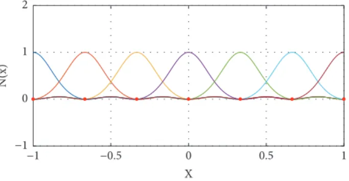
𝑁 + Λ𝑖𝑗. (21) Figures 1 and 2 depict the appearance of the simple Krig-ing interpolants usKrig-ing 7 control points uniformly distributed along the domain, for ℎ = 1 and ℎ = 1/3, respectively. It can be highlighted that both the Kronecker delta (i.e., strict interpolation) and the partition of unity properties are satisfied for any value ofℎ. Moreover, it is worth noting that the higher the variance the correlation function has, the more global the shape functions are. Furthermore, it is known that 99 per cent of the probability of a Gaussian distribution is comprised within an interval of[𝑚−3𝜎, 𝑚+3𝜎], being 𝑚 the mean value of the distribution. This issue explains perfectly well why the support of each Gaussian distribution takes 2 elements for the case, whereℎ = 1/3. Indeed, the shape of the interpolants is quite similar to standard finite element shape functions, but with a Gaussian profile. The remaining 1 per cent of probability is comprised in the small ridges happening in the middle of the elements.
In light of these results, a family of interpolants based on Kriging can be easily created just selecting the value of the variance within the correlation function. Therefore, globality of the support can be easily adjusted always under the framework of the partition of unity.
−1 0 1 2 N(x) −0.5 0 0.5 1 −1 X
Figure 1: Kriging shape functions using𝜎 = √(𝑥𝑖+1− 𝑥𝑖)2 for 7
control points uniformly distributed along the 1D domain.
−1 0 1 2 N(x) 0 0.5 1 −0.5 −1 X
Figure 2: Kriging shape functions using𝜎 = (1/3)√(𝑥𝑖+1− 𝑥𝑖)2for
7 control points uniformly distributed along the 1D domain.
2.4. Modal Adaptivity Strategy. In a standard PGD
frame-work, the final solution is approximated as a sum of𝑀 modes or functional products; see (2). Each one of the separated modes must be projected onto a chosen basis to render the problem finite dimensional. A standard choice is to select the same basis for each one of the modes:
N1= N2= ⋅ ⋅ ⋅ = N𝑀. (22) Despite of the fact that this choice seems reasonable, when dealing with nonstructured sparse data, it may not be such. In the previous section we proved that the rank of the separated system strongly depends on the distribution of the data sampling. Therefore, the cardinality of the interpolation basis must not exceed the maximum rank provided by the data sampling. Indeed, this constraint, which provides an upper bound to build the interpolation basis, only guarantees that the minimization is satisfied at the sampling points, without saying anything out of the measured points. Hence, if sampling points are not abundant, in the limit of low-data regime, high oscillations may appear out of these measured points. These oscillations are not desirable since the resulting prediction properties of the proposed method could be potentially decimated.
In order to tackle this problem, we take advantage of the residual-based nature of the PGD. Indeed, the greedy PGD algorithm tries to enrich a solution composed by𝑀 modes,
𝑢𝑀(𝑥, 𝑦) = ∑𝑀
𝑘=1
just by looking at the residual that accounts for the contribu-tion of the previous modes, as shown in 8).
Therefore, an appealing strategy to minimize spurious oscillations out of the sampling points is to start the PGD algorithm looking for modes with relatively smooth basis (for instance, Kriging interpolants with a few control points). Therefore, an indicator in order to make an online modal adaptive strategy is required. In the present work, we use the norm of the PGD residual,
R𝑀P = 1
√𝑃√𝑖∈P∑(𝑓 (𝑥𝑖, 𝑦𝑖) − 𝑢𝑀(𝑥𝑖, 𝑦𝑖))
2,
(24) whereP is the set of 𝑃 measured points and 𝑓(𝑥, 𝑦) is the function to be captured.
In essence, when the residual norm stagnates, a new control mesh is defined, composed by one more control point and always uniformly distributed, following
ΔR𝑀P = R𝑀P− R𝑀−1P < 𝜖𝑟. (25) By doing this, oscillations are reduced, since higher-order basis will try to capture only what remains in the residual. Here,𝜖𝑟is a tolerance defining the resilience of the sPGD to increase the cardinality of the interpolation basis. The lower 𝜖𝑟is, the more resilient method is to increase the cardinality.
To better understand the method, we will quantify the error for two set of points: the first set is associated with the sampling points,P, EP= #P1 ∑ 𝑠∈P √ (𝑓 (𝑥𝑠, 𝑦𝑠) − 𝑢𝑀(𝑥𝑠, 𝑦𝑠)) 2 𝑓 (𝑥𝑠, 𝑦𝑠)2 , (26) where𝑓(𝑥𝑠, 𝑦𝑠) is assumed not to vanish and where L also includes points other than the sampling points. This is done in order to validate the algorithm, by evaluating the reference solution—which is a priori unknown in a general setting—at points different to the sampling ones,
EL= #L1 ∑ s∈L
√ (𝑓 (𝑥𝑠, 𝑦𝑠) − 𝑢𝑀(𝑥𝑠, 𝑦𝑠))2
𝑓 (𝑥𝑠, 𝑦𝑠)2 . (27) Since the s-PGD algorithm minimizes the error only at the sampling pointsP it is reasonable to expect that EP ≤ EL.
2.5. A Preliminary Example. To test the convergence of the
just presented algorithm, we consider
𝑓1(𝑥, 𝑦) = (cos (3𝜋𝑥) + sin (3𝜋𝑦)) 𝑦2+ 4, (28)
which presents a quite oscillating behavior along the𝑥 direc-tion, whereas the𝑦 direction is quadratic. We are interested in capturing such a function in the domainΩ𝑦= Ω𝑥= [−1, 1]. Figures 3 and 4 show the errorsEPandELin identifying the function𝑓1(𝑥, 𝑦). In this case, we consider two distinct
sPGD (PGD points) sPGD (All points) 15 15.5 16 0 5 10 Er ro r [%] 5 10 15 20 25 0 # PGD Modes
Figure 3:EL (points) andEP (asterisk) versus the number of
modes for𝑓1(𝑥, 𝑦), #P = 100, #L = 1000. No modal adaptivity.
sPGD (PGD points) sPGD (All points) 5 10 15 20 0 5 10 Er ro r [%] 5 10 15 20 25 0 # PGD Modes
Figure 4: EL (points) andEP (asterisk) versus the number of
modes for𝑓1(𝑥, 𝑦), #P = 100, #L = 1000. Modal adaptivity based
on the residual,𝜖𝑟= 1e-2.
possibilities: no modal adaptivity at all and a modal adaptivity based on the residual, respectively. Several aspects can be highlighted. The first one is that EP (asterisks) decreases much faster when there is no modal adaptivity. This is expected, since we are minimizing with a richer basis since the very beginning, instead of starting with smooth functions like in the residual based approach. However, even if the min-imization in the sampling points is well achieved, when no modal adaptivity is considered, the error out of the sampling points may increase as the solution is enriched with new modes. Nevertheless, the residual-based modal adaptivity alleviates this problem. As it can be noticed, starting with relatively smooth functions drives the solution out of the sampling points to be smooth as well, avoiding the problem of high oscillations appearing out of the sampling points.
3. A Local Approach to s-PGD
It is well-known that, as in POD, reduced basis or, in general, any other linear model reduction technique, PGD gives poor results—in the form of a nonparsimonious prediction—when the solution of the problem lives in a highly nonlinear manifold. Previous approaches to this difficulty included the employ of nonlinear dimensionality reduction techniques such as Locally Linear Embeddings [22], kernel Principal
Component Analysis [23, 24] or isomap techniques [25]. Another, distinct, possibility, is to employ a local version of PGD [18], in which the domain is sliced so that at every sub-region PGD provides optimal or nearly optimal results. We explore this last option here for the purpose of sparse regres-sion, although a bit modified, as will be detailed hereafter.
The approach followed herein is based on the employ of the partition of unity property [26, 27]. In essence, it is well-known that any approximating function (like finite element shape functions, for instance) that forms a partition of unity can be enriched with an arbitrary function such that the resulting approximation inherits the smoothness of the partition of unity and the approximation properties of the enriching function.
With this philosophy in mind, we proposed to enrich a finite element mesh with an s-PGD approximation. The resulting approximation will be local, due to the compact support of finite element approximation, while inheriting the good approximation properties, already demonstrated, of s-PGD. In essence, what we propose is to construct an approximation of the type
𝑢 (𝑥, 𝑦) ≈ ∑ 𝑖∈I 𝑁𝑖(𝑥, 𝑦) 𝑢𝑖 + ∑ 𝑝∈Ienr ∑ 𝑒∈I𝑝 𝑁𝑒(𝑥, 𝑦)∑𝑀 𝑘=1 𝑋𝑘𝑝(𝑥) 𝑌𝑝𝑘(𝑦) ⏟⏟⏟⏟⏟⏟⏟⏟⏟⏟⏟⏟⏟⏟⏟⏟⏟⏟⏟⏟⏟⏟⏟⏟⏟⏟⏟⏟⏟⏟⏟ 𝑓enr 𝑝 (𝑥,𝑦) , (29) whereI represents the node set in the finite element mesh, Ienr the set of enriched nodes,𝑢𝑖 are the nodal degrees of freedom of the mesh,I𝑝 is the number of finite elements covered by node𝑝 shape function’s support and 𝑋𝑘𝑝(𝑥) and 𝑌𝑘
𝑝(𝑥) functions are the 𝑘-th one-dimensional PGD modes
enriching node𝑝, that in fact constitute an enriching function 𝑓enr(𝑥, 𝑦).
Of course, as already introduced in Eqs. (6) and (7), every PGD mode is in turn approximated by Galerkin projection on a judiciously chosen basis. In other words,
𝑢 (𝑥, 𝑦) ≈ ∑ 𝑖∈I 𝑁𝑖(𝑥, 𝑦) 𝑢𝑖 + ∑ 𝑝∈Ienr ∑ 𝑒∈I𝑝 𝑁𝑒(𝑥, 𝑦)∑𝑀 𝑘=1 (N𝑘𝑥)𝑇a𝑘𝑝(N𝑘𝑦)𝑇b𝑘𝑝, (30)
with a𝑘𝑝 and b𝑘𝑝 the nodal values describing each one-dimensional PGD mode.
In this framework, the definition of a suitable test func-tion can be done in several ways. As a matter of fact, the test function can be expressed as the sum of a finite element and a PGD contribution,
𝑢∗= 𝑢∗𝐹𝐸𝑀+ 𝑢∗𝑃𝐺𝐷, (31) so that an approach similar to that of Eq. (4) can be accomplished.
An example of the performance of this approach is included in Section 4.4. Linear Nearest Natural S-PGD SSL 0 5 10 15 20 Er ro r [%] 100 150 50 # Points
Figure 5: EL of𝑓1(𝑥, 𝑦) varying #P for different identification
techniques. #L = 1000.
4. Numerical Results
The aim of this section is to compare the ability of sparse model identification for different interpolation techniques. On one hand, the performance of standard techniques based on Delaunay triangulation such as linear, nearest neighbor or cubic interpolation is compared. Even though these techniques are simple, they allow to have a nonstructured sampling point set since they rely on a Delaunay triangu-lation. On the other hand, the results are compared to the Sparse Subspace Learning (SSL) [11]. The convergence and robustness of this method is proven to be very effective since the points are collocated at the Gauss-Lobato-Chebychev points. However, two main drawbacks appear considering this method. The first one is that there is a high concentration of points in the boundary of the domain, so that this quadrature is meant for functions that vary mainly along the boundary. Indeed, if the variation of the function appears in the middle of the domain, many sampling points will be required to converge to the exact function. The second one is that the sampling points have to be located at specific points in the domain. The s-PGD method using simple Kriging interpolants will be compared as well.
The numerical results are structured as follows: first two synthetic 2D functions are analyzed; secondly, two 2D response surfaces coming from a thermal problem and a Plastic Yield function are reconstructed; finally, a 10D synthetic function is reconstructed by means of the s-PGD algorithm.
4.1. 2D Synthetic Functions. The first considered function
is 𝑓1(𝑥, 𝑦), as introduced in the previous section. Figure 5 shows the reconstruction error (EL) of𝑓1(𝑥, 𝑦) for different sampling points. As it can be noticed, the s-PGD algorithm performs well for a wide range of sampling points. Neverthe-less, the SSL method is the one presenting the lower error level when there are more than 150 sampling points.
A second synthetic function is defined as
𝑓2(𝑥, 𝑦) = cos (3𝑥𝑦) + log (𝑥 + 𝑦 + 2.05) + 5. (32) This function is intended to be reconstructed in the domain Ω𝑥 = Ω𝑦 = [−1, 1]. It was chosen in such a way that it is
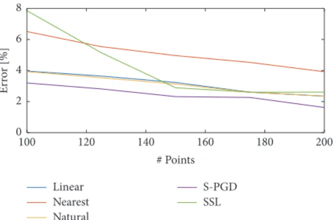
Linear Nearest Natural S-PGD SSL 30 40 50 60 20 # Points 0 2 4 6 8 Er ro r [%]
Figure 6:EL of𝑓2(𝑥, 𝑦) varying #P for different identification
techniques. #L = 1000.
relatively smooth in the center of the domain, whereas the main variation is located along the boundary of the domain. Indeed, this function is meant to show the potential of the SSL technique.
Figure 6 shows the reconstruction error of the𝑓2(𝑥, 𝑦) function for different interpolation techniques. As it can be noticed, both SSL and s-PGD methods are the ones that present the best convergence properties. If the number of points is increased even more, the SSL method is the one that presents the lowest interpolation error. They are followed by linear and natural neighbor interpolations. Finally, the nearest neighbor method is the one presenting the worst error for this particular case.
4.2. 2D Response Surfaces Coming from Physical Problems.
Once the convergence of the methods have been unveiled for synthetic functions, it is very interesting to analyze the power of the former methods by trying to identify functions that are coming from either simulations or models popular in the computational mechanics community. Indeed, two functions will be analyzed: the first one is an anisotropic Plastic Yield function, whereas the second one is a solution coming from a quasistatic thermal problem with varying source term and conductivity.
Figure 7 shows the Yld2004-18p anisotropic plastic yield function, defined by Barlat et al. in [28]. Under plane stress hypothesis, this plastic yield function is a convex and closed surface defined in a three-dimensional space. Therefore, the position vector of an arbitrary point in the surface can be easily parameterized in cylindrical coordinates as𝑅(𝜃, 𝜎𝑥𝑦). The 𝑅(𝜃, 𝜎𝑥𝑦) function for the Yld2004-18p is shown in Figure 8, where anisotropies can be easily seen. Otherwise, the radius function will be constant for a given𝜎𝑥𝑦.
Figure 9 shows the error in the identification of Barlat’s plastic yield function Yld2004-18p. As it can be noticed, the s-PGD technique outperforms the rest of techniques. Indeed, the s-PGD is exploiting the fact that the response surface is highly separable.
As mentioned above, the second problem is the sparse identification of the solution of a quasistatic thermal problem modeled by 0.5 0 −0.5 RS 0.5 0 −0.5 S R −1 0 1
Figure 7: Barlat’s Yld2004-18p function under plane stress hypoth-esis. 1.0 1 0.8 0.6 0.4 0.2 R RS 1 −1 0 1 −1 0
Figure 8:𝑅(𝜃, 𝜎𝑥𝑦) function for Barlat’s Yld2004-18p yield function.
∇ ⋅ (𝜂 (𝑥, 𝑡) ∇ (𝑢 (𝑥, 𝑡))) = 𝑓 (𝑡) ,
inΩ𝑥× Ω𝑡= [−1, 1] × [−1, 1] , (33) where conductivity varies in space-time as
𝜂 (𝑥, 𝑡) = (1 + 10 abs (𝑥) + 10𝑥2) log (𝑡 + 2.5)
𝑢 (1, 𝑡) = 2 (34)
𝑓 (𝑥, 𝑡) = 10 cos (3𝜋𝑡)
𝑢 (−1, 𝑡) = 2, (35)
and the source term varies in time. Homogeneous Dirichlet boundary conditions are imposed at both spatial boundaries and no initial conditions are required due to quasistationarity assumptions.
Figure 10 shows the evolution of the temperature field as a function of space time for the set of (33)-(35). It can be noticed how the variation of the temperature throughout time is caused mainly due to the source term. However, conductivity modifies locally the curvature of the temperature along the spatial axis. Symmetry with respect the𝑥 = 0 axis is preserved due to the fact that the conductivity presents a symmetry along the same axis.
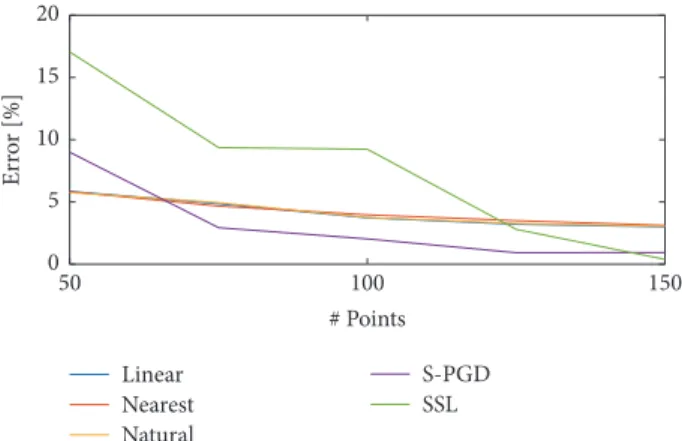
Figure 11 shows the performance of each one of the techniques when trying to reconstruct the temperature field from certain sampling points. As can be noticed, the s-PGD in conjunction with Kriging interpolants is the one that presents the fastest convergence rate to the actual function, which is considered unknown. It is followed by linear and natural interpolations. The SSL method presents a slow convergence rate in this case, due to the fact that the main variation of the function𝑢(𝑥, 𝑡) is happening in the center of the domain and not in the boundary.
Linear Nearest Natural S-PGD SSL 5 10 15 20 Er ro r [%] 80 100 120 140 160 60 # Points
Figure 9:ELof𝑅(𝜃, 𝜎𝑥𝑦) varying #P for different sparse
identifi-cation techniques. #L = 1000. 𝜖𝑟= 5 ⋅ 10−4. x 2.5 2 1.5 1 U 1 −1 0 1 −1 0t
Figure 10: Quasistatic solution to the thermal problem𝑢(𝑥, 𝑡).
4.3. A 10D Multivariate Case. In this subsection, we would
like to show the scalability that s-PGD presents when dealing with relatively high-dimensional spaces. Since our solution is expressed in a separated format, an𝑁 dimensional problem (𝑁𝐷) is solved as a sequence of 𝑁 1D problems, which are solved using a fixed-point algorithm in order to circumvent the nonlinearity of the separation of variables.
The objective function that we have used to analyze the properties of the s-PGD is defined as
𝑓3(𝑥1, 𝑥2, . . . , 𝑥𝑁) = 2 + 18∑𝑁 𝑖=1 𝑥𝑖+∏𝑁 𝑖=1 𝑥𝑖+∏𝑁 𝑖=1 𝑥2𝑖, (36) with𝑁 = 10 in this case.
Figure 12 shows the error convergence in both sampling points (EP, asterisks) and points out of the sampling (EL, filled points). TheL data set was composed by 3000 points, and theP data subset for the s-PGD algorithm was composed by 500 points. The number of points required to properly capture the hypersurface has increased with respect to the 2D examples due to the high dimensionality of the problem. Special attention has to be paid when increasing the cardi-nality of the interpolant basis without many sampling points, because the problem of high oscillations outside the control points may be accentuated.
4.4. An Example of the Performance of the Local s-PGD.
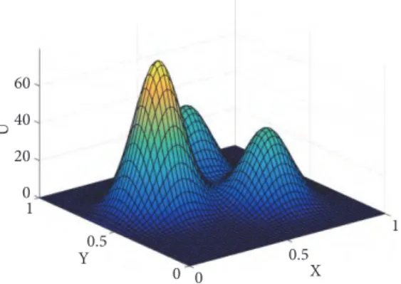
The last example corresponds to the sparse regression of an intricate surface that has been created by mixing three different Gaussian surfaces so as to generate a surface with
Linear Nearest Natural S-PGD SSL 120 140 160 180 200 100 # Points 0 2 4 6 8 Er ro r [%]
Figure 11:EL of𝑢(𝑥, 𝑡) varying #P for different identification
techniques. #L = 1000. 𝜖𝑟= 2.5 ⋅ 10−3. sPGD (PGD points) sPGD (All points) 1 1.5 2 2.5 3 0 5 10 Er ro r [%] 5 10 15 20 0 # PGD Modes
Figure 12:EL (points) and EP (asterisk) versus the number of
modes for 𝑓3(𝑥1, 𝑥2, . . . , 𝑥𝑁), #P = 500, #L = 3000. Modal
adaptivity based on the residual,𝜖𝑟= 1𝑒 − 3.
no easy separate representation (a nonparsimonious model, if we employ a different vocabulary). The appearance of this synthetic surface is shown in Figure 13.
The sought surface is defined in the domain Ω = [0, 1]2, which has been split into the finite element mesh shown in Figure 14. Every element in the mesh has been colored according to the number of enriching PGD functions, ranging from a single one to four. The convergence plot of this example as a function of the number of PGD modes added to the approximating space is included in Figure 15.
5. Conclusions
In this paper we have developed a data-based sparse reduced-order regression technique under the Proper Generalized Decomposition framework. This algorithm combines the robustness typical of the separation of variables together with properties of collocation methods in order to provide with parsimonious models for the data at hand. The performance of simple Kriging interpolation has proven to be effective when the sought model presents some regularity. Further-more, a modal adaptivity technique has been proposed in order to avoid high oscillations out of the sampling points, characteristic of high-order interpolation methods when data is sparse.
60 40 20 0 U Y 1 0.5 0 X 1 0.5 0
Figure 13: A synthetic surface generated by superposition of three different Gaussians, that is to be approximated by local s-PGD techniques. 0 0.5 1 X 0 0.5 1 Y 1 2 3 4
Figure 14: Finite element mesh for the example in Section 4.4. All the internal nodes have been enriched.
−3.6 −3.4 −3.2 −3 −2.8 −2.6 −2.4 log(Er ro r) 1.5 2 2.5 3 3.5 4 4.5 5 5.5 6 1 #Modes
Figure 15: Convergence plot for the example in Section 4.4.
For problems in which the result lives in a highly nonlinear manifold, a local version of the technique, which makes use of the partition of unity property, has also been developed. This local version outperforms the standard one for very intricate responses.
The s-PGD method has been compared advantageously versus other existing methods for different example func-tions. Finally, the convergence of s-PGD method for a high dimensional function has been demonstrated as well.
Although the sparsity of the obtained solution could not seem evident for the reader, we must highlight the fact
that the very nature of the PGD strategy a priori selects those terms on the basis that it plays a relevant role in the approximation. So to speak, PGD algorithms automatically discard those terms that in other circumstances will be weighted by zero. Sparsity, in this sense, is equivalent in this context to the number of sums in the PGD separated approximation. If only a few terms are enough to reconstruct the data—as is almost always the case—then sparsity is guaranteed in practice.
Sampling strategies other than the Latin hypercube method could be examined as well. This and the coupling with error indicators to establish good stopping criteria constitute our effort of research at this moment. In fact, the use of reliable error estimators could even allow for the obtention of adaptive samplings in which the cardinality of the basis could be different along different directions.
Data Availability
The data used to support the findings of this study are available from the corresponding author upon request.
Conflicts of Interest
The authors declare that they have no conflicts of interest.
Acknowledgments
This project has received funding from the European Union’s Horizon 2020 research and innovation program under the Marie Sklodowska-Curie Grant agreement no. 675919, also the Spanish Ministry of Economy and Competitiveness through Grants nos. DPI2017-85139-C2-1-R and DPI2015-72365-EXP, and the Regional Government of Aragon and the European Social Fund, research group T24 17R.
References
[1] T. Kirchdoerfer and M. Ortiz, “Data-driven computational mechanics,” Computer Methods Applied Mechanics and
Engi-neering, vol. 304, pp. 81–101, 2016.
[2] T. Kirchdoerfer and M. Ortiz, “Data driven computing with noisy material data sets,” Computer Methods Applied Mechanics
and Engineering, vol. 326, pp. 622–641, 2017.
[3] S. L. Brunton, J. L. Proctor, and J. N. Kutz, “Discovering govern-ing equations from data by sparse identification of nonlinear dynamical systems,” Proceedings of the National Acadamy of
Sciences of the United States of America, vol. 113, no. 15, pp. 3932–
3937, 2016.
[4] S. L. Brunton, J. L. Proctor, and J. N. Kutz, “Sparse identification of nonlinear dynamics with control (sindyc),” https://arxiv.org/abs/1605.06682.
[5] M. Quade, M. Abel, J. N. Kutz, and S. L. Brunton, “Sparse identification of nonlinear dynamics for rapid model recovery,”
Chaos: An Interdisciplinary Journal of Nonlinear Science, vol. 28,
no. 6, 063116, 10 pages, 2018.
[6] D. Gonzalez, F. Masson, F. Poulhaon, A. Leygue, E. Cueto, and F. Chinesta, “Proper generalized decomposition based dynamic
data driven inverse identification,” Mathematics and Computers
in Simulation, vol. 82, no. 9, pp. 1677–1695, 2012.
[7] B. Peherstorfer and K. Willcox, “Data-driven operator inference for nonintrusive projection-based model reduction,” Computer
Methods Applied Mechanics and Engineering, vol. 306, pp. 196–
215, 2016.
[8] D. Gonz´alez, F. Chinesta, and E. Cueto, “Thermodynamically consistent data-driven computational mechanics,” Continuum
Mechanics and Thermodynamics, 2018.
[9] N. M. Mangan, S. L. Brunton, J. L. Proctor, and J. N. Kutz, “Inferring Biological Networks by Sparse Identification of Non-linear Dynamics,” IEEE Transactions on Molecular, Biological,
and Multi-Scale Communications, vol. 2, no. 1, pp. 52–63, 2016.
[10] J. Mann and J. N. Kutz, “Dynamic mode decomposition for financial trading strategies,” Quantitative Finance, vol. 16, no. 11, pp. 1643–1655, 2016.
[11] D. Borzacchiello, J. V. Aguado, and F. Chinesta, “Non-intrusive Sparse Subspace Learning for Parametrized Problems,” Archives
of Computational Methods in Engineering: State-of-the-Art Reviews, pp. 1–24, 2017.
[12] C. Epstein, G. Carlsson, and H. Edelsbrunner, “Topological data analysis,” Inverse Problems, vol. 27, no. 12, 2011.
[13] W. Guo, K. Manohar, S. L. Brunton, and A. G. Banerjee, “Sparse-TDA: Sparse Realization of Topological Data Analysis for Multi-Way Classification,” IEEE Transactions on Knowledge and Data
Engineering, vol. 30, no. 7, pp. 1403–1408, 2018.
[14] F. Chinesta, A. Ammar, and E. Cueto, “Recent advances and new challenges in the use of the proper generalized decomposition for solving multidimensional models,” Archives of
Computa-tional Methods in Engineerin: State-of-the-Art Reviews, vol. 17,
no. 4, pp. 327–350, 2010.
[15] F. Chinesta, R. Keunings, and A. Leygue, The proper generalized
decomposition for advanced numerical simulations,
Springer-Briefs in Applied Sciences and Technology, Springer, Cham, 2014.
[16] F. Chinesta and P. Ladeveze, Eds., Separated representations and
PGD-based model reduction, vol. 554 of CISM International Centre for Mechanical Sciences. Courses and Lectures, Springer,
2014.
[17] D. Gonzalez, A. Ammar, F. Chinesta, and E. Cueto, “Recent advances on the use of separated representations,” International
Journal for Numerical Methods in Engineering, vol. 81, no. 5, pp.
637–659, 2010.
[18] A. Badas, D. Gonz´alez, I. Alfaro, F. Chinesta, and E. Cueto, “Local proper generalized decomposition,” International
Jour-nal for Numerical Methods in Engineering, vol. 112, no. 12, pp.
1715–1732, 2017.
[19] E. Cueto, D. Gonz´alez, and I. Alfaro, Proper generalized
decom-positions, Springer Briefs in Applied Sciences and Technology,
Springer, 2016.
[20] D. Gonz´alez, A. Badas, I. Alfaro, F. Chinesta, and E. Cueto, “Model order reduction for real-time data assimilation through extended Kalman filters,” Computer Methods Applied Mechanics
and Engineering, vol. 326, pp. 679–693, 2017.
[21] J.-C. Loiseau and S. L. Brunton, “Constrained sparse Galerkin regression,” Journal of Fluid Mechanics, vol. 838, pp. 42–67, 2018. [22] S. T. Roweis and L. K. Saul, “Nonlinear dimensionality reduc-tion by locally linear embedding,” Science, vol. 290, no. 5500, pp. 2323–2326, 2000.
[23] B. Sch¨olkopf, A. Smola, and K.-R. M¨uller, “Nonlinear compo-nent analysis as a kernel eigenvalue problem,” Neural
Computa-tion, vol. 10, no. 5, pp. 1299–1319, 1998.
[24] B. Scholkopf, A. Smola, and K. R. Muller, “Kernel principal component analysis,” in Advances in kernel methods - support
vector learning, pp. 327–352, MIT Press, 1999.
[25] J. B. Tenenbaum, V. de Silva, and J. C. Langford, “A global geometric framework for nonlinear dimensionality reduction,”
Science, vol. 290, no. 5500, pp. 2319–2323, 2000.
[26] J. M. Melenk and I. Babuˇska, “The partition of unity finite element method: basic theory and applications,” Computer
Methods Applied Mechanics and Engineering, vol. 139, no. 1–4,
pp. 289–314, 1996.
[27] I. Babuˇska and J. M. Melenk, “The partition of unity method,”
International Journal for Numerical Methods in Engineering, vol.
40, no. 4, pp. 727–758, 1997.
[28] J. W. Yoon, F. Barlat, R. E. Dick, and M. E. Karabin, “Prediction of six or eight ears in a drawn cup based on a new anisotropic yield function,” International Journal of Plasticity, vol. 22, no. 1, pp. 174–193, 2006.