Science Arts & Métiers (SAM)
is an open access repository that collects the work of Arts et Métiers Institute of
Technology researchers and makes it freely available over the web where possible.
This is an author-deposited version published in: https://sam.ensam.eu Handle ID: .http://hdl.handle.net/10985/10901
To cite this version :
Maxence BIGERELLE, Hakim NACEUR, Alain IOST - Analyses of the Instabilities in the Discretized Diffusion Equations via Information Theory - Entropy - Vol. 18, n°155, p.1-16 - 2016
Any correspondence concerning this service should be sent to the repository Administrator : [email protected]
entropy
Article
Analyses of the Instabilities in the Discretized
Diffusion Equations via Information Theory
Maxence Bigerelle1,*, Hakim Naceur1,†and Alain Iost2,†
1 LAMIH UMR CNRS 8201, Université de Valenciennes, Valenciennes 59313, France;
2 Laboratoire MSMP, Arts et Métiers ParisTech, Lille 59046, France; [email protected]
* Correspondence: [email protected]; Tel.: +33-6-16-297604
† These authors contributed equally to this work.
Academic Editor: Kevin H. Knuth
Received: 26 October 2015; Accepted: 12 April 2016; Published: 21 April 2016
Abstract:In a previous investigation (Bigerelle and Iost, 2004), the authors have proposed a physical interpretation of the instability λ =∆t/∆x2> 1/2 of the parabolic partial differential equations when solved by finite differences. However, our results were obtained using integration techniques based on erf functions meaning that no statistical fluctuation was introduced in the mathematical background. In this paper, we showed that the diffusive system can be divided into sub-systems onto which a Brownian motion is applied. Monte Carlo simulations are carried out to reproduce the macroscopic diffusive system. It is shown that the amount of information characterized by the compression ratio of information of the system is pertinent to quantify the entropy of the system according to some concepts introduced by the authors (Bigerelle and Iost, 2007). Thanks to this mesoscopic discretization, it is proved that information on each sub-cell of the diffusion map decreases with time before the unstable equality λ = 1/2 and increases after this threshold involving an increase in negentropy, i.e., a decrease in entropy contrarily to the second principle of thermodynamics.
Keywords: instability; entropy; parabolic partial differential equations; Monte Carlo simulations; data compression; information theory
PACS:89.70.Cf; 02.70.Bf; 05.10.Ln; 05.40.Jc
1. Introduction
Numerous physical phenomena can be modeled by partial differential equations (PDE) [1] and there are many numerical methods for solving PDE [2,3]. The Finite Element Method (FEM) and the Finite Volume Method (FVM) are particularly relevant to solve PDE. The FEM or FVM are mainly useful to solve PDE in complex geometries as well as to optimize the computation times by using different mesh sizes (or different discretization times). Among all these, the Finite Difference Method (FDM) stands out as being universally appropriate and straightforward for solving both linear and nonlinear problems, particularly for uniform mesh sizes and time increments. Stability criteria are analytically easily expressed for uniform mesh sizes and time increments. As the aim of this paper consists in analyzing criteria stability of PDE via Information theory, we deal exclusively with the FDM [4]. To solve these PDE numerically, FDM consists in expanding all variables of the PDE in a Taylor series on a grid at different points of the domain and to limit this expansion to the first derivatives. Then these finite expansions are introduced into the PDE problems and finally the algebraic system of equations is solved using adequate numerical algorithms. The main problems raised in this method are that PDE become discretized and all differential elements do not tend to 0 but to a fixed value that depends on the number of discretized points. However, discretization involves
Entropy 2016, 18, 155 2 of 16
local truncation errors and all rounding errors introduced during the computation due to the finite representation number might grow during the iterative process and leads to numerical instabilities. A high number of mathematical tools and theorems can be used to study the stability of the system, which we shall briefly summarize. However, no physical interpretation in term of Information theory has ever been proposed so far. The fundamental question can be summed up as follows: “Is there a link between the stability threshold and the quantity of information of the diffusive system at a given scale and how to quantify this amount of information?” Brillouin [5] proved that information could be considered as the negative of the system’s entropy called “Negentropy”. Entropy measures the lack of information; it gives the total amount of information missing in the ultramicroscopic structure of a system. In another scientific field, the Information theory can be a powerful tool to analyze data compression [6,7]. The more informative, the lower the ratio of data compression is. The discretized system will be integrally described if the size of the system after compression is minimal, regardless of the width of the data compression of all possible algorithms. Then the size of the program becomes a mathematical measure of negentropy. With regard to the numerous mathematical publications related to PDE stability, we propose to study the stability of parabolic PDE. Moreover, an important category of physical problems can easily be modeled at a microscopic scale and characterized by the Information theory concept via data compression [8].
2. Diffusion Equations
2.1. Parabolic Differential Equations
The Parabolic PDE is given by the following mathematical definition:
Bu Bt ´ n ÿ i,j B Bxi ai,j Bu Bxj “ f px, tq (1)
where px, tq PΩˆIR+, Ω an open set of IRn.
These equations characterize a high number of transport phenomena such as heat transfer, viscous fluid mechanics, transport of atoms-vacancies, Ohm law, contagious epidemics, etc. While remaining quite general, we shall treat in this investigation the simple mono-dimensional Fick Equation [9] that reduces Equation (1) to:
BC px, tq {Bt “ DB2C px, tq {Bx2 (2)
where C px, tq is the concentration of particles at position x after a time t and D is the diffusion coefficient. If we impose the initial condition, C p0, 0q “ C0δ0(explain what is δ0?) andΩ “ p´8, `8q, then the well-known solution is obtained:
C px, tq “ C0 2?πDtexp ˆ ´ x 2 4Dt ˙ (3)
This equation is in fact a Gaussian probability density function (if we substitute in Equation (3) C0by Equation (1) with zero mean and σ ptq “
?
2Dt standard deviation). Using Taylor’s expansion (explicit in time and central in space), we obtain:
Cij`1“Cij`D∆t{ p∆xq2 ”´
Ci´1j ´2Cij`Ci`1j ¯ı
(4)
where Cijrepresents the concentration at point x “ i∆x and time t “ j∆t.
Usually linear parabolic problems are solved via implicit or Crank–Nicolson’s schemes in order to avoid paying the price of the time step restriction. Unfortunately, implicit schemes (or mixed explicit/implicit schemes) involve that concentrations at time t `∆ t (partially or totally) depend on the gradients at time t `∆t. In 1905, Einstein proposed a physical explanation of D in Equation (2) by postulating that the concentration at time t `∆t only depends on the concentration at time t. Then
the explicit scheme will be retained because it is physically causal (i.e., evolution of the system only depends on previous time). It can be noticed that microscopic simulations of diffusion mechanisms are only explicit methods (Monte Carlo methods, Cellular automata, etc.).
2.2. Stability Study
In this Equation (4) scheme, concentration at time t `∆ t is calculated by means of the concentration at time t and then the explicit scheme becomes a dynamical system. As a result, it will be possible that this scheme becomes unstable for a set of values D∆t{ p∆xq2. The main idea behind stability is that a numerical process should limit the amplification of all components of the initial condition including rounding errors, when applied exactly. The basic analysis consider the growth of perturbations in initial data or the growth of errors introduced at mesh points at a given time level. This mathematical philosophy seems to us to be near the theory of chaos [10] and consequently we think that a duality exists between a mathematical interpretation and its physical representation. There are three common methods to investigate stability: the Von Neumann method, the matrix method, and the energy method. Using one of these three methods, it can be shown that the explicit scheme will be stable if [4]:
λ “D∆t{ p∆xq2ď1{2 (5)
2.3. Monte Carlo Simulation
The solution of the Cell-PDE could also be modeled using a Brownian motion. The discretization of the diffusion system takes place as follows. A grid of size rxˆry, rx “ry“ 256, is constructed. A 2D Monte Carlo (MC) simulation was used rather than a 1D one to visualize the complexity of the discretized diffusion front. In the middle of this grid, each elementary cell is affected to the value 1 on a length∆x “ rx{10 (good approximation, result not shown) that represents the entity (we shall call “particle”), which will diffuse; elsewhere, the value 0 is given (no particle). This system constitutes the initial state at time zero (original time). Figure1represents this initial state (t “ 0) where black cells represent the value “1” (particle) and white ones the value “0” (no particle).
Then, for each p particle, ns jumps are processed on the left or on the right with a probability of 1/2 (more precisely, a jump occurs by choosing at random one particle from all particles). This constitutes a Monte-Carlo Step (MCS). From the microscopic theory of diffusion [9], the diffusion coefficient D can be expressed by:
D “ a2Γ{2 (6)
whereΓ is the particle jump frequency of length a from one micro cell to one adjacent micro cell. The stability condition then can be expressed by including Equation (5) into Equation (6):
∆t p∆xq2 ď
1
a2Γ (7)
Then, the number of jumps nsover time∆ t is given by
ns“Γ∆t (8)
Without any lack of generality, we shall consider D “ 1. The elementary cell size is a “ 1 (pixel unit). Then the stability criterion becomes:
?
Entropy 2016, 18, 155 4 of 16 Entropy 2016, 18, 155 4 of 16 t = 0 t = 10 t = 300 <x> x concent ra tion 0 50 100 150 200 250 0 50 100 150 200 250 x conc ent rat ion 0 200 400 600 800 0 50 100 150 200 250 Monte carlo solution Gaussian solution x conc ent rat ion 0 50 100 150 0 50 100 150 200 250 Monte carlo solution Gaussian solution t = 655 t = 1000 x concentr ation 0 20 40 60 80 100 0 50 100 150 200 250 Monte carlo solution Gaussian solution x conc ent rat ion 0 20 40 60 80 0 50 100 150 200 250 Monte carlo solution Gaussian solution
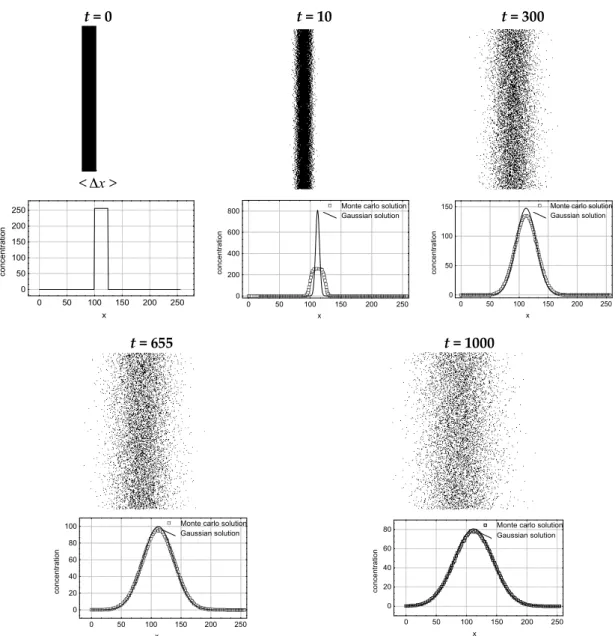
Figure 1. Snapshot of the Monte Carlo simulation for a grid size of 2552 at different Monte Carlo Steps (MCS) times (0, 10, 300, 655 (stability criterion), and 1000) and the concentration profiles under Gaussian approximation and given by the Monte Carlo method.
Figure 1 represents the snapshots of the evolution of the diffusion system at different times, 0, 10, 300, 655, 1000
s
n MCS. The particular value sc 2 (255 /10)2 655
s
n x corresponds to the
stability–instability threshold. Firstly, we shall verify the convergence rate of the Monte Carlo simulation to the Gaussian solution. Figure 1 shows also the concentration curves for different evolution times. The theoretical Gaussian curves given by Equation (3) are plotted for each concentration map. As can be observed, convergence to the Gaussian approximation is well suited if
300 s
n . Similar to these analyses, we shall develop and induce the Gaussian Probability Density Function approximation for the case ns nscs ; it becomes clear from the Monte-Carlo Simulation that the Gaussian PDF is an adequate assumption to model the diffusion process.
Figure 1. Snapshot of the Monte Carlo simulation for a grid size of 2552 at different Monte Carlo Steps (MCS) times (0, 10, 300, 655 (stability criterion), and 1000) and the concentration profiles under Gaussian approximation and given by the Monte Carlo method.
Figure1represents the snapshots of the evolution of the diffusion system at different times, ns “ 0, 10, 300, 655, 1000 MCS. The particular value nscs “ ∆x2 “ p255{10q2 “ 655 corresponds to the stability–instability threshold. Firstly, we shall verify the convergence rate of the Monte Carlo simulation to the Gaussian solution. Figure 1 shows also the concentration curves for different evolution times. The theoretical Gaussian curves given by Equation (3) are plotted for each concentration map. As can be observed, convergence to the Gaussian approximation is well suited if nsą300. Similar to these analyses, we shall develop and induce the Gaussian Probability Density Function approximation for the case ns“nscs ; it becomes clear from the Monte-Carlo Simulation that the Gaussian PDF is an adequate assumption to model the diffusion process.
3. Quantitative Description of the System in the Area of the Information Theory 3.1. Mathematical Formalism
The system X of diffusion states is an ordered set whose dimension dimpXq “ rxry“2562. This system contains sub-systems of the same dimension represented by xiwith length equal to∆x “ rx{10 and then dimpxiq “rxry{10 “ 2562{10.
Let us note T, the nonlinear bijective algebra that transforms the system x into a system y with y “ Tpxq. Let tAu be an algebraic set, Tminis said tAu -maxi contractile in X if there exists one algebra noted TminP tAu such that:
@x Ă X, @T P tAu , DTminP tAu , dimpTminpxqq ď dimpTpyqq (10)
Toptis said t8u -maxi contractile in X if Toptis tAu -maxi contractile in X where tAu denoted all the sets of all possible algebras defined by arithmetics. Regrettably, according to the Gödel incompleteness theorem, the proposition ! Topt is said t8u -maxi contractile in pES,Ψ, Gq " is undecidable [11] where pES,Ψ, Gq are, respectively, a vector space, the sets of all possible subspaces of ES, G a relation from ESto ES. However, a set of tAu algebra can be built and then ! tAu -maxi contractile in X " becomes decidable.
3.2. The Different Classes of Algebra
Run Length Encoding (RLE) is often used for data compression [12]. Each cell of the Monte-Carlo system is encoded by one bit, representing the existence or the absence of a particle. The efficiency of the RLE algorithm comes from the fact that selecting a cell at random, the probability that cells in the vicinity possess the same state is high under the hypothesis that physical system is not a pure random one (a pure random system possess the maximal statistical entropy). The algorithm counts the cells in rows on the grid looking for runs of cells having the same state. Encoding the number of runs rather than all individual states significantly reduces the initial size. Then we applied the Huffman algebra based on a list of the alphabetical symbols in decreasing probability order [13] on this system. This algebra allows us to better describe the structure of the diffusion that can be related to the probabilistic approach to this algebra (some statistical tools are closed to those used in statistical thermodynamics). This composition of both algebra denoted HUF ˝ RLEpXq is well adapted to describe the power laws met in the diffusion process [8,14].
4. Results
4.1. Compression Data Analyses
In the Monte Carlo simulation, the diffusive system Xptq is composed of 10 sub-systems xiptq with Xptq “ 10Y
i“1xiptq. At initial time t “ 0, the cells of the sub-system x5ptq are all equal to 1 and all the other sub-system cells are equal to 0. We shall analyze by the HUF ˝ RLE algebra the system X and the adjacent cells of x5, i.e., x4(or x6qthat are the cells that “received” the diffusion particles from the source located in x5. To integrate the stochastic aspect of the diffusion, 1000 simulations are carried out. At t “ 0, we get dimpHUF ˝ RLEpXqq “ 711 and dimpHUF ˝ RLEpx4qq “488 and these probability density functions are Dirac distributions (Figure2). As it can be shown, HUF ˝ RLE algebra is contractile on both X and x4systems because:
dimpHUF ˝ RLEpXp0qqq ă dimpXp0qq “ 65536 and dimpHUF ˝ RLEpx4p0qqq ă dimpx4p0qq “ 6554
Then, during the diffusion process (t ą 0), dimpHUF ˝ RLEpXptqqq and dimpHUF ˝ RLEpx4ptqqq follow Gaussian densities meaning that the stochastic variation of the Monte Carlo is detected by the RLE and Huffman algebra. If a diffusion system is finite, the concentration C px, tq will become a random variable that will follow a Gaussian law under a pure Brownian motion assumption [15].
Entropy 2016, 18, 155 6 of 16
The measure of the reduced space dimension follows the same density probability function meaning that an isomorphism exists between space dimension and the stochastic aspect of diffusion. As the diffusion time increases, dimpHUF ˝ RLEpXptqqq increases (Figure3): in fact, during the diffusion process, the total entropy increases, which will decrease negentropy. The system tends to disorder and information can be less and less reduced.
Entropy 2016, 18, 155 6 of 16
RLE and Huffman algebra. If a diffusion system is finite, the concentration C x t will become a
,random variable that will follow a Gaussian law under a pure Brownian motion assumption [15]. The measure of the reduced space dimension follows the same density probability function meaning that an isomorphism exists between space dimension and the stochastic aspect of diffusion. As the
diffusion time increases, dim(HUF RLE X t ( ( ))) increases (Figure 3): in fact, during the diffusion
process, the total entropy increases, which will decrease negentropy. The system tends to disorder and information can be less and less reduced.
t dim(HUF RLE X t ( ( ))) dim(HUF RLE x t ( ( )))4
0
Program size (in byte)
N
o of obs
650 675 700 725 750 775
Program size (in byte)
N o of obs 486 487 488 489 490 (a) (f) 10
Program size (in byte)
No of obs 0 100 200 300 1650 1700 1750 1800 1850 1900
Program size (in byte)
N o of obs 0 100 200 730 755 780 805 830 (b) (g) 300
Program size (in byte)
N o of obs 0 100 200 300 400 4520 4570 4620 4670 4720
Program size (in byte)
No of obs 0 100 200 300 1780 1800 1820 1840 1860 1880 (c) (h) 655
Program size (in byte)
No of obs 0 100 200 300 5300 5350 5400 5450
Program size (in byte)
No of obs 0 100 200 300 1860 1880 1900 1920 1940 1960 (d) (i) 1000
Program size (in byte)
No of obs 0 100 200 300 5640 5690 5740 5790 5840
Program size (in byte)
N o of obs 0 100 200 300 1830 1850 1870 1890 1910 1930 (e) (j)
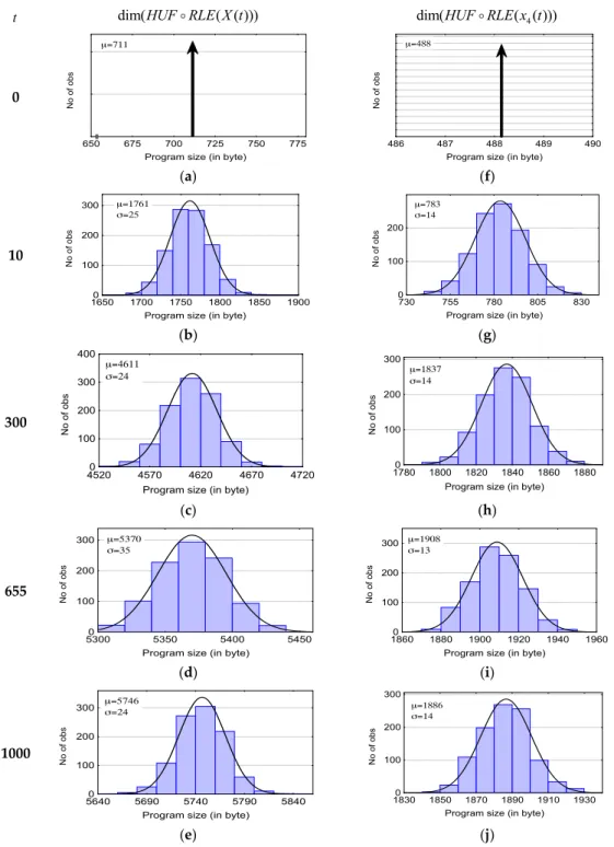
Figure 2. Histograms of the program sizes for the system X (a–e) and the sub system x4 (f–j)
corresponding to the Monte Carlo simulation for a grid size of 2552 at different MCS times (0, 10, 300,
Figure 2. Histograms of the program sizes for the system X (a–e) and the sub system x4 (f–j)
corresponding to the Monte Carlo simulation for a grid size of 2552 at different MCS times (0, 10,
300, 655 (stability criterion), and 1000). (a) Mean and standard deviation are computed and Gaussian density is plotted.
Entropy 2016, 18, 155 7 of 16
Entropy 2016, 18, 155 7 of 16
655 (stability criterion), and 1000). (a) Mean and standard deviation are computed and Gaussian density is plotted. time Dim(Huf.Rle(x4(t))) Dim(Huf.Rle(X(t))) 0 1000 2000 3000 4000 5000 6000 7000 200 400 600 800 1000 1200 1400 1600 1800 2000 0 1000 2000 3000 4000 5000 x4(t) X(t) 655
Figure 3. dim(HUF RLE X t ( ( ))) and dim(HUF RLE x t ( ( )))4 versus the diffusion time (in MCS)
for the grid size of 2552 cells (see Figure 1). Points are means of 40 simulations.
4.2. The Relation between Stability Criteria and the Dimension of Reduced Space
Now we shall analyze the evolution of the program size for the sub-space x . Figure 3 4
represents the evolution of the program size versus diffusion time.
First the dimension increases to reach a maximum and then decreases after this threshold. The diffusion time corresponding to this maximum is equal to tHUF RLEmax 65030 . This leads to an
important remark. Indeed, statistically:
max sc 2 (255 /10)2 655
HUF RLE s
t n x (11)
In the mono-dimensional diffusion problem, a PDE case gets two adjacent PDE cells that will diffuse on this cell. We shall consider particles coming from the adjacent cell. At the original time, no particle from the adjacent cell is present on the PDE cell and then the description of the cells can be summarized by an algorithmic formalism to “n rep 0” and then dim(HUF RLE x ( (0)))4 is minimal.
Then these particles will diffuse on the cell with respect to time. Then entropy will increase thanks to the diffusion and the amount of information will increase therefore increasing
4
dim(HUF RLE x ( (0))) until it reaches tHUF RLEmax that is the stability criterion (Figure 3). When the
diffusion time is higher than the stability threshold, then dim(HUF RLE x t ( ( )))4 decreases. This
means that there exists a link between the PDE stability criterion and the amount of information characterized by this original tool. We shall now give an explanation of the decrease in the dimension after the threshold criterion.
Now let us analyze very precisely this critical density function (Figure 4).
Figure 4. Three adjacent cells x x x1, ,2 3 of the discretized space grid x 1 on which mesoscopic
simulations are processed up to the instability criterion. Gaussian curves G1, G2 and G3 with standard
deviation of x 2Dt1 (D 1, t 1 / 2, i.e., 1 / 2) are centered on each cell.
x Fr equency 0 500 1000 1500 2000 2500 3000 -1 0 1 2 x1 x2 x3 x Dt G1 G2 G3 Dt
Figure 3.dimpHUF ˝ RLEpXptqqq and dimpHUF ˝ RLEpx4ptqqq versus the diffusion time (in MCS) for
the grid size of 2552cells (see Figure1). Points are means of 40 simulations.
4.2. The Relation between Stability Criteria and the Dimension of Reduced Space
Now we shall analyze the evolution of the program size for the sub-space x4. Figure3represents the evolution of the program size versus diffusion time.
First the dimension increases to reach a maximum and then decreases after this threshold. The diffusion time corresponding to this maximum is equal to tmaxHUF˝RLE “ 650˘30. This leads to an important remark. Indeed, statistically:
tmaxHUF˝RLE“nscs “∆x2“ p255{10q2“655 (11)
In the mono-dimensional diffusion problem, a PDE case gets two adjacent PDE cells that will diffuse on this cell. We shall consider particles coming from the adjacent cell. At the original time, no particle from the adjacent cell is present on the PDE cell and then the description of the cells can be summarized by an algorithmic formalism to “n rep 0” and then dimpHUF ˝ RLEpx4p0qqq is minimal. Then these particles will diffuse on the cell with respect to time. Then entropy will increase thanks to the diffusion and the amount of information will increase therefore increasing dimpHUF ˝ RLEpx4p0qqq until it reaches tmaxHUF˝RLEthat is the stability criterion (Figure3). When the diffusion time is higher than the stability threshold, then dimpHUF ˝ RLEpx4ptqqq decreases. This means that there exists a link between the PDE stability criterion and the amount of information characterized by this original tool. We shall now give an explanation of the decrease in the dimension after the threshold criterion.
Now let us analyze very precisely this critical density function (Figure4).
655 (stability criterion), and 1000). (a) Mean and standard deviation are computed and Gaussian density is plotted. time Dim(Huf.Rle(x4(t))) Dim(Huf.Rle(X(t))) 0 1000 2000 3000 4000 5000 6000 7000 200 400 600 800 1000 1200 1400 1600 1800 2000 0 1000 2000 3000 4000 5000 x4(t) X(t) 655
Figure 3. dim(HUF RLE X t ( ( ))) and dim(HUF RLE x t ( ( )))4 versus the diffusion time (in MCS)
for the grid size of 2552 cells (see Figure 1). Points are means of 40 simulations.
4.2. The Relation between Stability Criteria and the Dimension of Reduced Space
Now we shall analyze the evolution of the program size for the sub-space x . Figure 3 4
represents the evolution of the program size versus diffusion time.
First the dimension increases to reach a maximum and then decreases after this threshold. The diffusion time corresponding to this maximum is equal to tHUF RLEmax 65030. This leads to an
important remark. Indeed, statistically:
max sc 2 (255 /10)2 655
HUF RLE s
t n x (11)
In the mono-dimensional diffusion problem, a PDE case gets two adjacent PDE cells that will diffuse on this cell. We shall consider particles coming from the adjacent cell. At the original time, no particle from the adjacent cell is present on the PDE cell and then the description of the cells can be summarized by an algorithmic formalism to “n rep 0” and then dim(HUF RLE x ( (0)))4 is minimal.
Then these particles will diffuse on the cell with respect to time. Then entropy will increase thanks to the diffusion and the amount of information will increase therefore increasing
4
dim(HUF RLE x ( (0))) until it reaches tHUF RLEmax that is the stability criterion (Figure 3). When the
diffusion time is higher than the stability threshold, then dim(HUF RLE x t ( ( )))4 decreases. This
means that there exists a link between the PDE stability criterion and the amount of information characterized by this original tool. We shall now give an explanation of the decrease in the dimension after the threshold criterion.
Now let us analyze very precisely this critical density function (Figure 4).
Figure 4. Three adjacent cells x x x1, ,2 3 of the discretized space grid x 1 on which mesoscopic
simulations are processed up to the instability criterion. Gaussian curves G1, G2 and G3 with standard
deviation of x 2Dt1 (D 1, t 1 / 2, i.e., 1 / 2) are centered on each cell.
x Fr equency 0 500 1000 1500 2000 2500 3000 -1 0 1 2 x1 x2 x3 x Dt G1 G2 G3 Dt
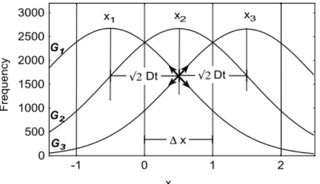
Figure 4. Three adjacent cells x1, x2, x3of the discretized space grid∆x “ 1 on which mesoscopic
simulations are processed up to the instability criterion. Gaussian curves G1, G2and G3with standard
deviation of∆x “?2Dt “ 1 (D “ 1, t “ 1{2, i.e., λ “ 1{2) are centered on each cell.
Let us now consider the x2intervals. Concentration is the summation of all the Gaussian curves on these intervals and the concentration on the x2cell only results from the flux from cells x1and x3.
Entropy 2016, 18, 155 8 of 16
For the condition∆x “?2Dt, the inflexion points of the Gaussians G1and G3are in the middle of the interval x2. Then the following expressions can be stated:
B2C1,0 ´ x,∆x2{2D,∆x¯{Bx2ă0, B2C3,0 ´ x,∆x2{2D,∆x¯{Bx2ą0 @x P rx2´∆x{2, x2s (12) B2C1,0 ´ x2,∆x2{2D,∆x ¯ {Bx2“0, B2C3,0 ´ x2,∆x2{2D,∆x ¯ {Bx2“0 (13) B2C1,0 ´ x,∆x2{2D,∆x¯{Bx2ą0, B2C3,0 ´ x,∆x2{2D,∆x¯{Bx2ă0 @x P rx2, x2`∆x{2s (14) From Equation (2), B2C
i,jpx, t,∆xq {Bx29BCi,jpx, t,∆xq {B t and it can be concluded that 50% of dx micro intervals (dx !∆x) of x2intervals get a positive temporal gradient (BC1,0px, t,∆xq {Bt ą 0 and BC3,0px, t,∆xq {Bt ą 0), and 50% a negative gradient (BC1,0px, t,∆xq {Bt ă 0 and BC3,0px, t,∆xq {Bt ă 0). After the stability threshold, more than 50% of micro cells get a negative gradient. This clearly means that particles issued from adjacent cells x1 and x3 will decrease in keeping with time, which will decrease the configuration entropy of the system x2contrarily to the second principle of thermodynamics for a diffusive system. The mathematical criterion of stability of the explicit scheme is then physically related to the production of entropy characterized by our algebra operator: if the scheme is unstable, then the production of entropy on each discretized cell is negative and the size of the program will decrease.
We eventually get: BdimpHUF ˝ RLEpx4ptqqq{Bt ą 0 if ? 2Dt ă∆x, t ą 0 (15) BdimpHUF ˝ RLEpx4ptqqq{Bt “ 0 if ? 2Dt “∆x (16) BdimpHUF ˝ RLEpx4ptqqq{Bt ă 0 if ? 2Dt ą∆x (17)
To illustrate these partial differential equations, different system sizes are simulated using the Monte Carlo diffusion process (from s = 250 to 1000). Then, according to Equation (11), and if assertion ! tHUF ˝ RLEu -maxi contractile in X " is true, the relation between the threshold that depends on the system size (because the system is always decomposed into 10 sub-systems with parts of equal length) becomes:
tmaxHUF˝RLEpsq “ nscs psq “∆x2psq “ ps{10q2 (18)
Figure5represents the normalized dimension obtained by dimpHUF ˝ RLEpx4ptqqq{dimpx4ptqq for the different system sizes. The maximal values for each system size are computed and compared to Equation (18).
As can be observed, data match to the theoretical equation meaning that whatever the system size, the time of maximal entropy tmaxHUF˝RLEpsq is obtained so that it corresponds to the stability criterion. Thanks to statistical thermodynamics, it was shown that stability threshold corresponding to a violation of the second principle of the thermodynamics that confirms all results shown by the Information theory tools [16].
Entropy 2016, 18, 155 9 of 16
Figure 5. dim(HUF RLE x t ( ( ))) / dim( ( ))4 x t4 versus the diffusion time (in MCS) for different grid
sizes of cells (250, 300, …, 950, 1000). Values of the time tHUF RLEmax are plotted (graph on the right
corner) versus the theoretical stability criterion nscs ( / 10)s 2 given by Equation (18).
5. Two Examples of PDE
5.1. Non Constant Diffusion Coefficient
The problems treated by the information theory were investigated with a constant diffusion coefficient. In this case, the diffusion coefficient does not depend on the position. Thus, we will treat the following problem:
,
, C x t D x C x t t x x (19)For a real positive diffusion parameter D(x) that depends on the x-position, the classical explicit first order in time and second order in space method in the one-dimensional case is stable if:
2 max 1/ 2 D x t x (20)The x-dependence of diffusion coefficient D can be due to different variations of material properties like crystal structure, local molar concentration, vacancy gradient, etc., or external conditions like residual stress, temperature, electrical field, chemical potential, etc.
A positive perturbation a x( ) is introduced to the unitary jump length during the Brownian simulation process and the mean displacement of each particle becomes 1 a x( ). By posing
( ) 1 ( )
a x a x in Equation (7), one gets D x( )
a x( )
2 and the local stability criterion becomes:
( ) / (1 ( ))
s
n x x a x (21)
Finally, the global stability criterion becomes:
min / (1 ( ))
s x
n x a x (22)
A Gaussian function will be used to simulate the variation of diffusion coefficient:
2 1 2 ( , , ) x c a x c e (23) time normalized dimension 0 0.005 0.01 0.015 0.02 0.025 0.03 0 5000 10000 15000 20000 700 750 800 400 450 500 550 600 650 250 300 350 850 900 950 1000 theoretical time modelized tme 0 2000 4000 6000 8000 10000 12000 0 2500 5000 7500 10000 System size:
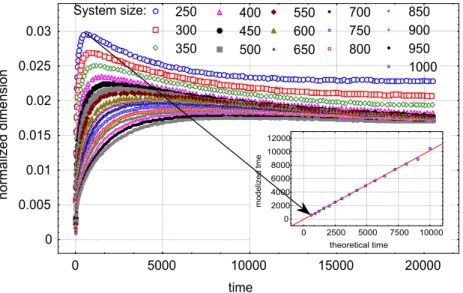
Figure 5.dimpHUF ˝ RLEpx4ptqqq{dimpx4ptqq versus the diffusion time (in MCS) for different grid sizes
of cells (250, 300, . . . , 950, 1000). Values of the time tmaxHUF˝RLEare plotted (graph on the right corner)
versus the theoretical stability criterion nscs “ ps{10q2given by Equation (18).
5. Two Examples of PDE
5.1. Non Constant Diffusion Coefficient
The problems treated by the information theory were investigated with a constant diffusion coefficient. In this case, the diffusion coefficient does not depend on the position. Thus, we will treat the following problem:
B BtC px, tq “ B BxD pxq B BxC px, tq (19)
For a real positive diffusion parameter D(x) that depends on the x-position, the classical explicit first order in time and second order in space method in the one-dimensional case is stable if:
λ “ max pD pxqq∆t
p∆xq2 ď1{2 (20)
The x-dependence of diffusion coefficient D can be due to different variations of material properties like crystal structure, local molar concentration, vacancy gradient, etc., or external conditions like residual stress, temperature, electrical field, chemical potential, etc.
A positive perturbation∆apxq is introduced to the unitary jump length during the Brownian simulation process and the mean displacement of each particle becomes 1 `∆apxq. By posing apxq “ 1 `∆apxq in Equation (7), one gets Dpxq “ papxqq2and the local stability criterion becomes:
a
nspxq ď p∆x{p1 ` ∆apxqqq (21)
Finally, the global stability criterion becomes: ?
nsďmin
x p∆x{p1 ` ∆apxqqq (22)
A Gaussian function will be used to simulate the variation of diffusion coefficient:
∆apx, c, σq “ e12px´cσ q 2
Entropy 2016, 18, 155 10 of 16
To assess nonlinearity, the size of the system is increased and resolution map will be extended to N = 1024 (rather than N = 256 for the previous simulations). The Gaussian is centered at 3/4 of the diffusion map and then c = 3 ˆ 1024/4 = 768 (Figure6).
Entropy 2016, 18, 155 10 of 16
To assess nonlinearity, the size of the system is increased and resolution map will be extended to N = 1024 (rather than N = 256 for the previous simulations). The Gaussian is centered at 3/4 of the diffusion map and then c = 3 × 1024/4 = 768 (Figure 6).
x (in pixels)
a( x, c, ) 0 200 400 600 800 1000 0.0 0.2 0.4 0.6 0.8 1.0 =12 2 2 2 2 2 2 2 2 2Figure 6. Values of a x c( , , ) exp 0.5
x c
2/2 versus x for different standard deviations σ.These functions allow producing nonlinear PDEs involving different stability criteria
( , , ) / 1 ( , , ) s
n x c x a x c along the x position for a given pair( , )c .
The mesh size is equal to x 1024 / 8 128 . At t = 0, the diffusion cell is located the middle of the map (at t = 0, xi,j = 1 j
1,1024
if i belongs to i4 = [448,576] otherwise xi,j = 0). The diffusion only occurs in the x direction. Figure 7 represents snapshots of the diffusion process for two standard deviations. As can be observed, for the standard deviation of 112 pixels, a dissymmetry of the concentration appears and diffusion increases on the right of the diffusion map. Contrarily, diffusion map is symmetrical for diffusion map obtained with small standard deviation (and for high standard deviation, i.e., greater than 220 pixels, result not shown). According to Equation (21), for very small standard deviations, one gets:
2 ² 0 ( , , ) 128 16384, , ,lim
n x csx
x c (24)and for high standard deviations, one gets:
2( , , ) / 4 4096, ,
lim
n x csx
x c
(25)
In these two cases, diffusion becomes linear and stability condition does not depend on x position. Let us now analyze the two compression ratio, dim(HUF RLE i t ( ( ))) / dim( ( ))n i tn , of the two adjacent cells (i3, i5) at i4 (i3 = [320,448], i5 = [576,704]) for different values of standard deviations (Figure 8). As can be observed, all curves present maximal values of compression leading to a MCS time sc( , , )
s
n x c that depend on the values of the standard deviations.
Figure 6. Values of∆apx, c, σq “ exp0.5 px ´ cq2{σ2 versus x for different standard deviations σ.
These functions allow producing nonlinear PDEs involving different stability criteriaanspx, c, σq ď
∆x{ p1 ` ∆apx, c, σqq along the x position for a given pairpc, σq.
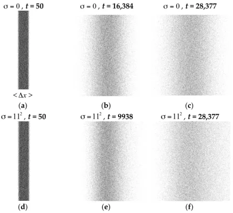
The mesh size is equal to∆x “ 1024{8 “ 128. At t = 0, the diffusion cell is located the middle of the map (at t = 0, xi,j= 1 @j P r1, 1024s if i belongs to i4= [448,576] otherwise xi,j= 0). The diffusion only occurs in the x direction. Figure7represents snapshots of the diffusion process for two standard deviations. As can be observed, for the standard deviation of 112 pixels, a dissymmetry of the concentration appears and diffusion increases on the right of the diffusion map. Contrarily, diffusion map is symmetrical for diffusion map obtained with small standard deviation (and for high standard deviation, i.e., greater than 220pixels, result not shown). According to Equation (21), for very small standard deviations, one gets:
lim
σÑ0pnspx, c, σqq ď∆x 2
“1282“16384, @x, @c, (24)
and for high standard deviations, one gets:
lim
σÑ8pnspx, c, σqq ď∆x
2{4 “ 4096, @x, @c (25)
In these two cases, diffusion becomes linear and stability condition does not depend on x position. Let us now analyze the two compression ratio, dimpHUF ˝ RLEpinptqqq{dimpinptqq, of the two adjacent cells (i3, i5) at i4 (i3= [320,448], i5= [576,704]) for different values of standard deviations (Figure8). As can be observed, all curves present maximal values of compression leading to a MCS time nscs px, c, σq that depend on the values of the standard deviations.
Entropy 2016, 18, 155 11 of 16 0 , t = 50 0, t = 16,384 0, t = 28,377 <x> (a) (b) (c) 2 11 , t = 50 112, t = 9938 112, t = 28,377 (d) (e) (f)
Figure 7. Snapshots of the Monte Carlo simulation for a grid size of 10242 pixels at different Monte
Carlo Steps (MCS) times (50, stability criterion, 28,377). (a) 0, t = 50; (b) 0, t = 16,384;
(c) 0, t = 28,377; (d) 112, t = 50; (e) 112, t = 9938; (f) 112, t = 28,377. MCS Time N o rm al iz ed D im ens io n 5 50 500 5000 50000 0.02 0.04 0.06 0.08 0.10 0.12 0.14 0.16 =0 =12 =22 =32 =42 =52 =62 =72 =82 =92 =102 =112 =122 =132 =142 =152 =162 =172 =182 =192 =202
Figure 8. dim(HUF RLE i t ( ( ))) / dim( ( ))5 i t5 versus the diffusion time (in MCS) for different values of standard deviations.
From our postulate, the theoretical stability criterion is equal to
2( , , ) / (1 ( , , )) sc
s
n x c x a x c . Values of the theoretical stability threshold agree with simulated
values (Figure 9), meaning that our method can be applied to linear PDE with non-constant diffusion coefficient.
Figure 7.Snapshots of the Monte Carlo simulation for a grid size of 10242pixels at different Monte
Carlo Steps (MCS) times (50, stability criterion, 28,377). (a) σ “ 0, t = 50; (b) σ “ 0, t = 16,384; (c) σ “ 0,
t = 28,377; (d) σ “ 112, t = 50; (e) σ “ 112, t = 9938; (f) σ “ 112, t = 28,377. Entropy 2016, 18, 155 11 of 16 0 , t = 50 0, t = 16,384 0, t = 28,377 <x> (a) (b) (c) 2 11 , t = 50 112, t = 9938 112, t = 28,377 (d) (e) (f)
Figure 7. Snapshots of the Monte Carlo simulation for a grid size of 10242 pixels at different Monte
Carlo Steps (MCS) times (50, stability criterion, 28,377). (a) 0, t = 50; (b) 0, t = 16,384;
(c) 0, t = 28,377; (d) 112, t = 50; (e) 112, t = 9938; (f) 112, t = 28,377. MCS Time N o rm al iz ed D im ens io n 5 50 500 5000 50000 0.02 0.04 0.06 0.08 0.10 0.12 0.14 0.16 =0 =12 =22 =32 =42 =52 =62 =72 =82 =92 =102 =112 =122 =132 =142 =152 =162 =172 =182 =192 =202
Figure 8. dim(HUF RLE i t ( ( ))) / dim( ( ))5 i t5 versus the diffusion time (in MCS) for different values of standard deviations.
From our postulate, the theoretical stability criterion is equal to
2( , , ) / (1 ( , , )) sc
s
n x c x a x c . Values of the theoretical stability threshold agree with simulated
values (Figure 9), meaning that our method can be applied to linear PDE with non-constant diffusion coefficient.
Figure 8.dimpHUF ˝ RLEpi5ptqqq{dimpi5ptqq versus the diffusion time (in MCS) for different values of
standard deviations.
From our postulate, the theoretical stability criterion is equal to
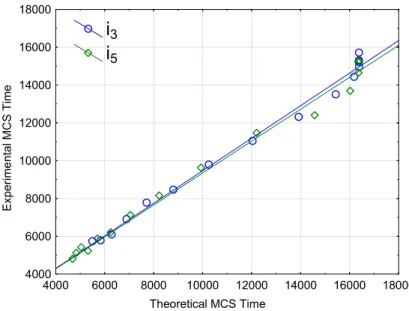
nscs px, c, σq “ p∆x{p1 ` ∆apx, c, σqqq2. Values of the theoretical stability threshold agree with simulated values (Figure9), meaning that our method can be applied to linear PDE with non-constant diffusion coefficient.
Entropy 2016, 18, 155 12 of 16 Entropy 2016, 18, 155 12 of 16 Theoretical MCS Time Ex per im e ntal M C S T ime 4000 6000 8000 10000 12000 14000 16000 18000 4000 6000 8000 10000 12000 14000 16000 18000
i
3i
5Figure 9. Plot of MCS tHUF RLEmax versus the theoretical stability criterion
2( ) / (1 ( ))
sc s
n x x a x
given by Equation (21) for both cells i4 and i5 corresponding to maximal values of Figure 8.
5.2. Nonlinear PDE
The problems treated by the information theory were investigated on a linear PDE. A vast array of complex phenomena of motion, reaction, diffusion, equilibrium, conservation, and more lead to nonlinear PDE. A PDE is said to be nonlinear if the relations between the unknown functions and their partial derivatives involved in the equation are nonlinear. Thus, we will treat the following nonlinear problem:
,
,
, C x t D C x t C x t t x x (26)In our case, the diffusion coefficient depends on the concentration C x t
, . Lee [17] proposed diffusion coefficients relating to the uptake of excess calcium by calcium chloride [18]. The diffusion coefficient D takes the form:
,
0
1 , D D C x t aC x t (27)where a is a coefficient that represents sur-diffusion processes (a < 0) or a sub-diffusion ones (a > 0) or a classical diffusion ones (a = 0). In our simulations, a
1, 0,1, 2,3, 4,5
. The stability criterion is given by:
2 max , 1/ 2 D C x t t x (28)The Monte Carlo simulation is based on an explicit scheme. Jump length at time t + dt is computed from concentration at time t (Figure 10). Too validate our hypothesis, 50 simulations are performed with three sizes of the system: 1282, 2562 and 5122 pixels. Maximal values of the dimension are extracted (Figure 11).
Figure 9.Plot of MCS tmax
HUF˝RLEversus the theoretical stability criterion nscs pxq “ p∆x{p1 ` ∆apxqqq2
given by Equation (21) for both cells i4and i5corresponding to maximal values of Figure8.
5.2. Nonlinear PDE
The problems treated by the information theory were investigated on a linear PDE. A vast array of complex phenomena of motion, reaction, diffusion, equilibrium, conservation, and more lead to nonlinear PDE. A PDE is said to be nonlinear if the relations between the unknown functions and their partial derivatives involved in the equation are nonlinear. Thus, we will treat the following nonlinear problem: B BtC px, tq “ B BxD pC px, tqq B BxC px, tq (26)
In our case, the diffusion coefficient depends on the concentration C px, tq. Lee [17] proposed diffusion coefficients relating to the uptake of excess calcium by calcium chloride [18]. The diffusion coefficient D takes the form:
D pC px, tqq “ D0
1 ` aC px, tq (27)
where a is a coefficient that represents sur-diffusion processes (a < 0) or a sub-diffusion ones (a > 0) or a classical diffusion ones (a = 0). In our simulations, a “ t´1, 0, 1, 2, 3, 4, 5u. The stability criterion is given by:
λ “ max pD pC px, tqqq∆t
p∆xq2 ď1{2 (28)
The Monte Carlo simulation is based on an explicit scheme. Jump length at time t + dt is computed from concentration at time t (Figure10). Too validate our hypothesis, 50 simulations are performed with three sizes of the system: 1282, 2562 and 5122pixels. Maximal values of the dimension are extracted (Figure11).
Entropy 2016, 18, 155 13 of 16 Entropy 2016, 18, 155 13 of 16 a −1 0 1 2 3 4 t = 5 MCS Instability Threshold 300 MCS 600 MCS 1000 MCS 1300 MCS 1600 MCS 2000 MCS
Figure 10. Snapshots of the nonlinear Monte Carlo simulation for a grid size of 1292 pixels at five
Monte Carlo Steps (MCS) times with different values of a given by D C x t
,
D0
1aC x t
,
and snapshots corresponding to stability criterion and their associated Monte Carlo Steps.
Figure 11. dim(HUF RLE i t ( ( ))) / dim( ( ))5 i t5 versus the diffusion time (in MCS) for different
values of diffusion coefficient D C x t
,
D0
1aC x t
,
.Values of the theoretical stability threshold agree with simulated values (Figure 12), meaning that our method can be applied to nonlinear PDE.
Theoretical MCS time Ex pe rim ent al M C S tim e 300 400 500 600 700 800 900 1000 2000 3000 4000 5000 6000 7000 8000 9000 10000 20000 30000 40000 50000 100 300 500 700 900 2000 4000 6000 8000 10000 30000 50000 Size 129² 257² 512²
Figure 12. Plot of MCS tHUF RLEmax versus the theoretical stability criterion for both cells i4 and i5
corresponding to maximal values of Figure 11 (Size = 2572) and Size = (1292, 5122).
MCS Time N o rm al iz ed D im e n si o n 0 22 47 78 129 231 468 1065 2616 6697 17492 0.02 0.04 0.06 0.08 0.10 0.12 0.14 a -1 0 1 2 3 4 5
Figure 10. Snapshots of the nonlinear Monte Carlo simulation for a grid size of 1292pixels at five
Monte Carlo Steps (MCS) times with different values of a given by D pC px, tqq “ D0{ p1 ` aC px, tqq
and snapshots corresponding to stability criterion and their associated Monte Carlo Steps.
Entropy 2016, 18, 155 13 of 16 a −1 0 1 2 3 4 t = 5 MCS Instability Threshold 300 MCS 600 MCS 1000 MCS 1300 MCS 1600 MCS 2000 MCS
Figure 10. Snapshots of the nonlinear Monte Carlo simulation for a grid size of 1292 pixels at five
Monte Carlo Steps (MCS) times with different values of a given by D C x t
,
D0
1aC x t
,
and snapshots corresponding to stability criterion and their associated Monte Carlo Steps.
Figure 11. dim(HUF RLE i t ( ( ))) / dim( ( ))5 i t5 versus the diffusion time (in MCS) for different
values of diffusion coefficient D C x t
,
D0
1aC x t
,
.Values of the theoretical stability threshold agree with simulated values (Figure 12), meaning that our method can be applied to nonlinear PDE.
Theoretical MCS time Ex pe rim ent al M C S tim e 300 400 500 600 700 800 900 1000 2000 3000 4000 5000 6000 7000 8000 900010000 20000 30000 40000 50000 100 300 500 700 900 2000 4000 6000 8000 10000 30000 50000 Size 129² 257² 512²
Figure 12. Plot of MCS tHUF RLEmax versus the theoretical stability criterion for both cells i4 and i5
corresponding to maximal values of Figure 11 (Size = 2572) and Size = (1292, 5122).
MCS Time N o rm al iz ed D im e n si o n 0 22 47 78 129 231 468 1065 2616 6697 17492 0.02 0.04 0.06 0.08 0.10 0.12 0.14 a -1 0 1 2 3 4 5
Figure 11.dimpHUF ˝ RLEpi5ptqqq{dimpi5ptqq versus the diffusion time (in MCS) for different values of
diffusion coefficient D pC px, tqq “ D0{ p1 ` aC px, tqq.
Values of the theoretical stability threshold agree with simulated values (Figure12), meaning that our method can be applied to nonlinear PDE.
a −1 0 1 2 3 4
t = 5 MCS
Instability Threshold
300 MCS 600 MCS 1000 MCS 1300 MCS 1600 MCS 2000 MCS
Figure 10. Snapshots of the nonlinear Monte Carlo simulation for a grid size of 1292 pixels at five
Monte Carlo Steps (MCS) times with different values of a given by D C x t
,
D0
1aC x t
,
and snapshots corresponding to stability criterion and their associated Monte Carlo Steps.
Figure 11. dim(HUF RLE i t ( ( ))) / dim( ( ))5 i t5 versus the diffusion time (in MCS) for different
values of diffusion coefficient D C x t
,
D0
1aC x t
,
.Values of the theoretical stability threshold agree with simulated values (Figure 12), meaning that our method can be applied to nonlinear PDE.
Theoretical MCS time Ex pe rim ent al M C S tim e 300 400 500 600 700 800 900 1000 2000 3000 4000 5000 6000 7000 8000 9000 10000 20000 30000 40000 50000 100 300 500 700 900 2000 4000 6000 8000 10000 30000 50000 Size 129² 257² 512²
Figure 12. Plot of MCS tmaxHUF RLE versus the theoretical stability criterion for both cells i4 and i5
corresponding to maximal values of Figure 11 (Size = 2572) and Size = (1292, 5122).
MCS Time N o rm al iz ed D im e n si o n 0 22 47 78 129 231 468 1065 2616 6697 17492 0.02 0.04 0.06 0.08 0.10 0.12 0.14 a -1 0 1 2 3 4 5
Figure 12. Plot of MCS tmaxHUF˝RLE versus the theoretical stability criterion for both cells i4 and i5
Entropy 2016, 18, 155 14 of 16
6. Discussion
To summarize, the mathematical criterion of stability λ “∆t{∆x2ą1{2 of the explicit scheme leads to an unstable scheme due to the decrease of information versus time characterized by the reduction size of the system on each discretized cell of the whole system. In the stability vision of Von Neumann, a finite difference scheme is stable if the errors made at one time step of the calculation do not let the errors increase for the following time steps. Therefore, in our approach, this means that, for a fixed time of observation of the diffusion, an increase of the size of the sub-cells of the grid will irrevocably lead to a critical size from which discretized information will not be enough to contain information on concentration gradient described by the partial differential equation. In fact, the physical interpretation of instability of the PDE was never introduced in a high number of papers, which treat mathematical aspects of instability via information formalisms. Mishra has introduced the problems of violation of local thermodynamic laws in the transport equations via Information theory. He discretizes the transport equation via a simple centered finite difference scheme. The time derivative is replaced with a forward difference and the spatial derivative with a central difference. In this scheme of discretization, the central scheme leads to a growth of energy at every time step and is unstable whatever the size of both discretization of time and space [19]. Mishra explains why the solutions computed with the central scheme blow up. After all, the central scheme seems a reasonable approximation of the transport equation. The physical explanation can be deduced from the following argument: the exact solution moves to the right with entities speed (Figure13).
Entropy 2016, 18, 155 14 of 16
6. Discussion
To summarize, the mathematical criterion of stability t x2 1 2 of the explicit scheme leads to an unstable scheme due to the decrease of information versus time characterized by the reduction size of the system on each discretized cell of the whole system. In the stability vision of Von Neumann, a finite difference scheme is stable if the errors made at one time step of the calculation do not let the errors increase for the following time steps. Therefore, in our approach, this means that, for a fixed time of observation of the diffusion, an increase of the size of the sub-cells of the grid will irrevocably lead to a critical size from which discretized information will not be enough to contain information on concentration gradient described by the partial differential equation. In fact, the physical interpretation of instability of the PDE was never introduced in a high number of papers, which treat mathematical aspects of instability via information formalisms. Mishra has introduced the problems of violation of local thermodynamic laws in the transport equations via Information theory. He discretizes the transport equation via a simple centered finite difference scheme. The time derivative is replaced with a forward difference and the spatial derivative with a central difference. In this scheme of discretization, the central scheme leads to a growth of energy at every time step and is unstable whatever the size of both discretization of time and space [19]. Mishra explains why the solutions computed with the central scheme blow up. After all, the central scheme seems a reasonable approximation of the transport equation. The physical explanation can be deduced from the following argument: the exact solution moves to the right with entities speed (Figure 13).
Figure 13. The central scheme used by Mishra [20] to illustrate physical interpretation of the
unconditional instability of the simple centered finite difference scheme. Continuous arrows (green) indicate numerical propagation and dashed ones arrows (magenta) physical propagation.
Unfortunately, for the scheme described in this publication that we have physically proof to be physical relevant in term of the physics causality via Einstein theory of the Brownian motion [15], no justification of the conditional stabilities was found in the bibliography via Information theory. However, some results using entropy concept in PDE stability conclude [21] that many linear Partial Differential Equations or Integral equations with non-constant coefficients satisfy some entropy dissipation properties [22]. Finally, explicit time discretization leads to entropy production [23] and more specifically, explicit scheme with Lax–Friedrichs flux is entropy stable under conditions given by Equation (5) [24].
7. Conclusions
In this paper, we showed that a relation exists between the well-known stability criterion
2/ 1/ 2
D t x
applied on the explicit numerical scheme Cxtt Cit
Cxtx2CxtCxtx
to guarantee the convergence of the 1D non-stationary PDE C x t
, / t D C x t2
, /x2 to the solution and the quantity of information contained at a mesoscopic scale under the size of discretization x. Implicit and semi implicit schemes (such as the unconditionally stable scheme of Crank–Nicolson method) lead to a violation of the principle of causality: the cause must precede its effect according to all inertial observers meaning that the cause and its effect are separated by a time-like interval, and the effect belongs to the future of its cause. Jaroszkiewicz pointed out the violation of causality in the fields of discrete mechanics by analyzing the implicit and explicit EulerFigure 13. The central scheme used by Mishra [20] to illustrate physical interpretation of the unconditional instability of the simple centered finite difference scheme. Continuous arrows (green) indicate numerical propagation and dashed ones arrows (magenta) physical propagation.
Unfortunately, for the scheme described in this publication that we have physically proof to be physical relevant in term of the physics causality via Einstein theory of the Brownian motion [15], no justification of the conditional stabilities was found in the bibliography via Information theory. However, some results using entropy concept in PDE stability conclude [21] that many linear Partial Differential Equations or Integral equations with non-constant coefficients satisfy some entropy dissipation properties [22]. Finally, explicit time discretization leads to entropy production [23] and more specifically, explicit scheme with Lax–Friedrichs flux is entropy stable under conditions given by Equation (5) [24].
7. Conclusions
In this paper, we showed that a relation exists between the well-known stability criterion λ “D∆t{ p∆xq2ď1{2 applied on the explicit numerical scheme Ct`x ∆t“Cit` λ
´
Cx´∆xt ´2Ctx`Cx`∆xt ¯
to guarantee the convergence of the 1D non-stationary PDE BC px, tq {Bt “ DB2C px, tq {Bx2 to the solution and the quantity of information contained at a mesoscopic scale under the size of discretization ∆ x. Implicit and semi implicit schemes (such as the unconditionally stable scheme of Crank–Nicolson method) lead to a violation of the principle of causality: the cause must precede its effect according to all inertial observers meaning that the cause and its effect are separated by a time-like interval, and the effect belongs to the future of its cause. Jaroszkiewicz pointed out the violation of causality in the
fields of discrete mechanics by analyzing the implicit and explicit Euler Schemes and deduced that the implicit scheme involves that the flow of information occurs in a temporal loop. Jaroszkiewicz concluded his argument with the following question: “we should ask, given this violation of causal implication, how could we ever use implicit Euler scheme in practical calculation” [25]. Under Causality scheme assumptions, it was proved that instability occurs during iterative process if and only if information contained inside the cell∆x decreases with time, thus violating the second principle of the thermodynamics. As microscopic simulations of diffusion mechanisms are only explicit methods (Monte Carlo methods, Cellular automata, etc.), the criterion of sub-cell information seems to be a relevant tool to assess that a stable explicit scheme meets both the causality and the second principle of the thermodynamics.
Author Contributions: Maxence Bigerelle found the concept of negentropy production in explicit numerical scheme. Alain Iost applied this to material science. Hakim Naceur formulated the explicit scheme. All authors have read and approved the final manuscript.
Conflicts of Interest:The authors declare no conflict of interest.
References
1. Dautray, R.; Lions, J.-L. Analyse Mathématique et Calcul Numérique pour les Sciences et les Techniques. Volume 1:
Modèles Physiques; Masson: Paris, France, 1987. (In French)
2. Dautray, R.; Lions, J.-L. Analyse Mathématique et Calcul Numérique pour les Sciences et les Techniques. Volume 7:
Evolution, Fourier, Laplace; Masson: Paris, France, 1988. (In French)
3. Dautray, R.; Lions, J.-L. Analyse Mathématique et Calcul Numérique pour les Sciences et les Techniques. Tome 9:
Evolution, Numérique, Transport; Masson: Paris, France, 1997. (In French)
4. Forsythe, G.E.; Wasow, W.R. Finite Difference Methods for Partial Differential Equations; Wiley: New York, NY,
USA, 1960.
5. Brillouin, L. Science and Information Theory; Academic Press: New York, NY, USA, 1956.
6. Delahaye, J.P. Information, Complexité Hasard; Hermès: Paris, France, 1994. (In French)
7. Chaitin, G.J. Algorithmic Information Theory; Cambridge University Press: Cambridge, UK, 1887.
8. Bigerelle, M.; Iost, A. Relations entre l’entropie physique, le codage de l’information et l’énergie de simulation.
Can. J. Phys. 2007, 85, 1381–1394. (In French) [CrossRef]
9. Adda, Y.; Philibert, J. La Diffusion Dans les Solides, Tome II; Presses Universitaires de France: Paris, France, 1966.
10. Peitgen, H.O.; Jürgens, H.; Saupe, D. Chaos and Fractals: New Frontiers of Science; Springer: New York, NY,
USA, 1992.
11. Feferman, J.W. Kurt Gödel Collected Works. Volume 1: Publications, 1929–1936; Oxford University Press: Oxford,
UK, 1986.
12. Salomon, D. Data Compression; Springer: New York, NY, USA, 1998.
13. Huffman, D. A method for the construction of minimum redundancy codes. Proc. IRE 1952, 40, 1098–1101.
[CrossRef]
14. Bigerelle, M.; Iost, A. Relationship between information reduction and the equilibrium state description.
Comput. Mater. Sci. 2002, 24, 133–138. [CrossRef]
15. Einstein, A. Investigation on the Theory of Brownian Motion; Dover Publications: New York, NY, USA, 1956.
16. Bigerelle, M.; Iost, A. Physical interpretation of the numerical instabilities in diffusion equations via statistical
thermodynamics. Int. J. Nonlinear Sci. Numer. Simul. 2004, 5, 121–134. [CrossRef]
17. Lee, C.F. On the solution of some diffusion equations with concentration-dependent diffusion coefficients—II.
IMA J. Appl. Math. 1972, 10, 129–133. [CrossRef]
18. Wagner, C. Diffusion processes during the uptake of excess calcium by calcium fluoride. J. Phys. Chem. Solids
1968, 29, 1925–1930. [CrossRef]
19. Mishra, S.; Veerappa Gowda, G.D. Optimal entropy solutions for conservation laws with discontinuous
flux-functions. J. Hyperbolic Differ. Equ. 2005, 2, 783–837.
20. Mishra, S. Numerical Methods for Conservation Laws and Related Equations. Available online:
https://www2.math.ethz.ch/education/bachelor/lectures/fs2013/math/nhdgl/numcl_notes_HOMEPAGE.pdf (accessed on 14 April 2016).
Entropy 2016, 18, 155 16 of 16
21. Tadmor, E. Entropy stability theory for difference approximations of nonlinear conservation laws and related
time-dependent problems. Acta Numer. 2003, 12, 451–512. [CrossRef]
22. Carrillo, J.A.; Jüngel, A.; Markowich, P.A.; Toscani, G.; Unterreiter, A. Entropy dissipation methods for
degenerate parabolic problems and generalized sobolev inequalities. Monatshefte für Mathematik 2001, 133,
1–82. [CrossRef]
23. Lefloch, P.G.; Mercier, J.M.; Rohde, C. Fully discrete, entropy conservative schemes of arbitrary order. SIAM J.
Numer. Anal. 2002, 40, 1968–1992. [CrossRef]
24. Noble, P.; Vila, J.P. Stability theory for difference approximations of some dispersive shallow water equations
and application to thin film flows. 2013, arXiv:1304.3805.
25. Jaroszkiewicz, G. Principles of Discrete Time Mechanics; Cambridge University Press: Cambridge, UK, 2014.
© 2016 by the authors; licensee MDPI, Basel, Switzerland. This article is an open access article distributed under the terms and conditions of the Creative Commons Attribution (CC-BY) license (http://creativecommons.org/licenses/by/4.0/).

![Figure 13. The central scheme used by Mishra [20] to illustrate physical interpretation of the unconditional instability of the simple centered finite difference scheme](https://thumb-eu.123doks.com/thumbv2/123doknet/7346567.212675/15.892.251.641.543.684/figure-illustrate-physical-interpretation-unconditional-instability-centered-difference.webp)
