Pépite | La réponse de la communauté phytoplanctonique aux changements globaux et leurs effets sur le fonctionnement de l'écosystème avec une attention particulière à Phaeocystis spp, une algue nuisible

Texte intégral

(1)Thèse de Stéphane Karasiewicz, Lille 1, 2017. École Doctorale Sciences de la Matière, du Rayonnement et de l’Environnement Spécialité Géoscience, Ecologie, Paléontologie, Océanographie.. Université de Lille 1 Laboratoire d’Océanologie et de Géosciences UMR 8187 LOG Equipe 1 : Diversité, processus et interactions dans les écosystèmes marins. The phytoplankton community response(s) to global changes and their effect(s) on ecosystem functioning with a special focus on Phaeocystis spp, a harmful algae. Thèse de doctorat présentée par. Stéphane KARASIEWICZ Soutenue publiquement le 22 Décembre 2017 devant le jury composé de : Directeur de thèse Sébastien LEFEBVRE, Professeur, Université Lille 1 Rapporteurs Valérie DAVID, Maître de conférences, Université de Bordeaux Koen SABBE, Professeur, Université de Gand, Belgique Examinateurs Annie CHAPELLE, Docteur, IFREMER, Brest Christine DUPUY, Professeur, Université de la Rochelle Dorothé VINCENT, Maître de conférences, ULCO Stéphane DRAY, Directeur de Recherche, Université de Lyon I. © 2017 Tous droits réservés.. lilliad.univ-lille.fr.

(2) Thèse de Stéphane Karasiewicz, Lille 1, 2017. © 2017 Tous droits réservés.. lilliad.univ-lille.fr.

(3) Thèse de Stéphane Karasiewicz, Lille 1, 2017. École Doctorale Sciences de la Matière, du Rayonnement et de l’Environnement Spécialité Géoscience, Ecologie, Paléontologie, Océanographie.. Université de Lille 1 Laboratoire d’Océanologie et de Géosciences UMR 8187 LOG Equipe 1 : Diversité, processus et interactions dans les écosystèmes marins. The phytoplankton community response(s) to global changes and their effect(s) on ecosystem functioning with a special focus on Phaeocystis spp, a harmful algae. Thèse de doctorat présentée par. Stéphane KARASIEWICZ Soutenue publiquement le 22 Décembre 2017 devant le jury composé de : Directeur de thèse Sébastien LEFEBVRE, Professeur, Université Lille 1 Rapporteurs Valérie DAVID, Maître de conférences, Université de Bordeaux Koen SABBE, Professeur, Université de Gand, Belgique Examinateurs Annie CHAPELLE, Docteur, IFREMER, Brest Christine DUPUY, Professeur, Université de la Rochelle Dorothé VINCENT, Maître de conférences, ULCO Stéphane DRAY, Directeur de Recherche, Université de Lyon I. © 2017 Tous droits réservés.. lilliad.univ-lille.fr.


(5) Thèse de Stéphane Karasiewicz, Lille 1, 2017. Je dédicace cette thèse à mes parents, Diane et Daniel KARASIEWICZ, qui ont su me soutenir et savent que je viens de loin pour en arriver là.. © 2017 Tous droits réservés.. lilliad.univ-lille.fr.


(7) Thèse de Stéphane Karasiewicz, Lille 1, 2017. «Science is beautiful when it makes simple explanations of phenomena or connections between different observations. ». -Stephen Hawking. © 2017 Tous droits réservés.. lilliad.univ-lille.fr.


(9) Thèse de Stéphane Karasiewicz, Lille 1, 2017. Remerciements Je tiens à remercier en tout premier lieu Valérie DAVID et Koen SABBE pour avoir accepté d’être rapporteurs de cette thèse ainsi que Annie CHAPELLE, Christine DUPUY, Dorothé VINCENT et Stéphane DRAY examinateurs de ce travail. Merci à Sébastien Lefebvre, mon directeur de thèse, de m’avoir accepté en tant qu’ étudiant en thèse, sachant que je n’étais pas encore titulaire de mon Master. Merci de m’avoir formé à ce métier de chercheur afin que je puisse maintenant, et je le cite, «m’envoler de mes propres ailes.». Je voudrais également remercier mes coauteurs Sylvain DOLÉDEC, Elsa BRETON, Alain LEFEBVRE et Tania HERNÁNDEZ-FARIÑAS, pour leur remarques et critiques pertinentes qui m’ont permis de publier deux articles. Merci à François SCHMITT, directeur du Laboratoire d’Océanologie et Géosciences, de m’avoir ouvert les portes de son laboratoire. Merci aux autres personnels du laboratoire, notamment ceux de la Station Marine que j’ai le plus côtoyé. Je souhaiterais aussi remercier mes collègues de bureau, qui se reconnaitront, pour la fabuleuse ambiance et qui ont su apporter au quotidien... Je voudrais personnellement remercier mes parents, Diane et Daniel KARASIEWICZ, qui ont toujours cru en moi, même durant les périodes les plus difficile de mes études. De m’avoir soutenu, moralement et financièrement, lorsque j’étais à l’étranger. Mes sœurs, Natacha et Tania, qui ont aussi su m’aider et trouver les mots justes à des moments clefs. Elles ne pourront plus dire que leur frère est le rois des ...s mais qu’il a réussi malgré toutes les galères qu’il a eu. Je souhaiterais aussi remercier Julie LOWMAN et Elaine METCALFE, qui avec ma mère, ont lu et corrigé les fautes d’anglais de cette thèse. Sans oublier Yann pour ton pain-bouchon, les amis (les vrais) ,qui ne liront surement jamais ma thèse mais, qui sont toujours là après toutes ces années et avec qui on rigole toujours autant. Enfin, je tiens fortement à remercier Carolina GIRALDO LOPEZ, pour son soutien quotidien indéfectible, ses succulents petits plats, mais surtout sa patience et son écoute qui ont été indispensable à l’aboutissement de cette thèse.. © 2017 Tous droits réservés.. lilliad.univ-lille.fr.


(11) Thèse de Stéphane Karasiewicz, Lille 1, 2017. 0.1. RÉSUMÉ. 0.1. i. Résumé. Les écosystèmes côtiers, interfaces entre terre et mer, sont soumis au changement climatique ainsi qu’à de fortes pressions anthropiques. La plupart des eaux côtières sont sujettes à l’eutrophisation, en conséquence de ces activités. Le phytoplancton fait l’objet d’une attention particulière en raison de sa position entant que producteur primaire des écosystèmes marins. Récemment, l’efflorescence des algues nuisibles (HAB) est devenu une préoccupation croissante, dans le monde entier. L’objectif de la thèse a été de décrire et de mesurer les réponses temporelles et les causalités de la structure de communauté phytoplanctonique sous impacts des changements globaux et de l’ occurrence d’une algue nuisible. Pour ce faire, le concept de niche écologique et une méthode statistique, ont été adaptés. Les "Within Outlying Mean Indexes" (WitOMI) ont ensuite été proposés pour affiner l’analyse de l’ "Outlying Mean Index" en combinant ses propriétés avec la décomposition de la marginalité de l’analyse "K-select". Les dynamics des sous-niches des espèces de la communauté ont été étudiées dans des conditions environnementales contrastées d’ abondances basses (L) ou fortes (H) de Phaeocystis spp. Le sous-ensemble H était caractérisé par une large niche de Phaeocystis spp. ainsi qu’une haute diversité de diatomées. Dans le sous-ensemble L, la sous-niche de Phaeocystis spp. a était soumis à une forte contrainte biologique possiblement crée par la compétition pour les ressources par les diatomées. Dans ces conditions environmentales, la relation diversité-productivité du phytoplancton a été étudié à court et long termes. Cette relation s’est avérée plus forte à l’échelle saisonnière. Le déséquilibre des ressources n’a pas eu de lien direct avec la productivité sur le modèle à long terme. Le succès à long terme de l’espèce invasive et de son impact sur la productivité, peut être expliqué par des années froides successives avec des ressources plus élevées mais déséquilibrées, ce qui augmente le nombre de petites espèces de diatomées favorisant son efflorescence. Enfin, je discute des améliorations méthodologiques possibles, du potentiel et de l’intérêt de l’utilisation de l’approches par traits, et d’éventuelles configurations expérimentales afin de renforcer les résultats de la thèse. © 2017 Tous droits réservés.. lilliad.univ-lille.fr.

(12) Thèse de Stéphane Karasiewicz, Lille 1, 2017. ii. 0.2. Abstract. Coastal ecosystems, the interfaces between land and sea, are subject to climate change and high anthropogenic pressure. Most coastal waters are prone to eutrophication, as a consequence of the subsequent human activities. The phytoplankton is the subject of special attention because of its position as a primary producer in marine ecosystems. Recently, Harmful Algae Bloom (HAB) outbreaks has become an increasing concern around the world. The aim of the thesis was to describe and to measure the temporal responses and causalities of the phytoplankton community structure, with the occurrence of a harmful algae, under global changes. To do so, the ecological niche concept along with a statistical method were adapted. The Within Outlying Mean Indexes (WitOMI) was then proposed to refine the Outlying Mean Index analysis by using its properties in combination with the K-select analysis species marginality decomposition. The subniche dynamic of the community species was studied under environmental conditions hosting low (L) and high (H) Phaeocystis spp. abundance. Subset H was characterized by a large Phaeocystis spp. niche and a high diatom diversity. In subset L, Phaeocystis spp. subniche was subject to great biological constrain suspected to be caused by diatom competition for resources. In these environmental conditions, the phytoplankton diversityproductivity relationship is expected to vary in the short and long-terms. This relationship was stronger at a seasonal scale. The resource imbalance had no direct link with productivity in the long term model. The long-term invasive species success and its impact on productivity can be explained by successive cold years with higher resource imbalance, which increased the number of small diatom species favoring its bloom. I finally discussed on the possible methodological improvements, the potential interest of using the "trait-based approach", and possible experimental set-ups to reinforce the result of the thesis.. © 2017 Tous droits réservés.. lilliad.univ-lille.fr.

(13) Thèse de Stéphane Karasiewicz, Lille 1, 2017. Contents. 0.1. Résumé . . . . . . . . . . . . . . . . . . . . . . . . . . . . . . .. i. 0.2. Abstract . . . . . . . . . . . . . . . . . . . . . . . . . . . . . . .. ii. General introduction. 1. 1.1. Generalities on phytoplankton ecology . . . . . . . . . . . . . .. 1. 1.2. Global change . . . . . . . . . . . . . . . . . . . . . . . . . . . .. 6. 1.2.1. Temperature effects on phytoplankton . . . . . . . . . .. 7. 1.2.2. Eutrophication . . . . . . . . . . . . . . . . . . . . . . .. 9. 1.3. Harmful Algae . . . . . . . . . . . . . . . . . . . . . . . . . . . . 11 1.3.1. Generalities . . . . . . . . . . . . . . . . . . . . . . . . . 11. 1.3.2. An invasive species: Phaeocystis spp. . . . . . . . . . . . 12. 1.4. Link between diversity and productivity . . . . . . . . . . . . . 13. 1.5. Niche concept . . . . . . . . . . . . . . . . . . . . . . . . . . . . 16. 1.6. Problematic . . . . . . . . . . . . . . . . . . . . . . . . . . . . . 17. Materials and Methods. 19. 2.1. Data . . . . . . . . . . . . . . . . . . . . . . . . . . . . . . . . . 19. 2.2. Community analysis . . . . . . . . . . . . . . . . . . . . . . . . 20. 2.3. Niche analysis . . . . . . . . . . . . . . . . . . . . . . . . . . . . 21. 2.4. 2.3.1. Species frequency table . . . . . . . . . . . . . . . . . . . 22. 2.3.2. Subniche parameters calculated from the origin G . . . . 23. 2.3.3. Subniche parameters calculated from a sub-origin GK . . 25. Structural Equation Modelling . . . . . . . . . . . . . . . . . . . 27 2.4.1. Description and approaches . . . . . . . . . . . . . . . . 27. 2.4.2. Model evaluation . . . . . . . . . . . . . . . . . . . . . . 29. Within Outlying Mean Indexes: refining the OMI analysis for the realized niche decomposition. 31 3.1. Introduction . . . . . . . . . . . . . . . . . . . . . . . . . . . . . 31. 3.2. The Within Outlying Mean Indexes (WitOMI) concept . . . . . 37. 3.3. © 2017 Tous droits réservés.. 3.2.1. Statistical significance . . . . . . . . . . . . . . . . . . . 38. 3.2.2. Graphical display . . . . . . . . . . . . . . . . . . . . . . 38. Ecological application . . . . . . . . . . . . . . . . . . . . . . . . 39 3.3.1. Temporal subniche dynamics . . . . . . . . . . . . . . . . 39. 3.3.2. Spatial subniche dynamics . . . . . . . . . . . . . . . . . 41 iii. lilliad.univ-lille.fr.

(14) Thèse de Stéphane Karasiewicz, Lille 1, 2017. iv. CONTENTS 3.4. Discussion . . . . . . . . . . . . . . . . . . . . . . . . . . . . . . 42. 3.5. Acknowledgements . . . . . . . . . . . . . . . . . . . . . . . . . 48. Environmental response of Phaeocystis spp. realized niche. 49. 4.1. Introduction . . . . . . . . . . . . . . . . . . . . . . . . . . . . . 49. 4.2. Methods . . . . . . . . . . . . . . . . . . . . . . . . . . . . . . . 51. 4.3. 4.4. 4.2.1. Data set . . . . . . . . . . . . . . . . . . . . . . . . . . . 51. 4.2.2. Subsets creation . . . . . . . . . . . . . . . . . . . . . . . 52. 4.2.3. Niche and subniche analysis . . . . . . . . . . . . . . . . 53. 4.2.4. Biological constraint . . . . . . . . . . . . . . . . . . . . 53. Results . . . . . . . . . . . . . . . . . . . . . . . . . . . . . . . . 54 4.3.1. Subset habitat conditions . . . . . . . . . . . . . . . . . 54. 4.3.2. Niche analysis (OMI) . . . . . . . . . . . . . . . . . . . . 56. 4.3.3. Subniche calculations (WitOMI) . . . . . . . . . . . . . . 59. 4.3.4. Biological reducing factor . . . . . . . . . . . . . . . . . 62. Discussion . . . . . . . . . . . . . . . . . . . . . . . . . . . . . . 64 4.4.1. Phaeocystis spp.hypotheses . . . . . . . . . . . . . . . . . 64. 4.4.2. Biotic interactions . . . . . . . . . . . . . . . . . . . . . 65. 4.4.3. Further perspectives . . . . . . . . . . . . . . . . . . . . 67. 4.5. Conclusion . . . . . . . . . . . . . . . . . . . . . . . . . . . . . . 68. 4.6. Acknowledgements . . . . . . . . . . . . . . . . . . . . . . . . . 68. Phytoplankton long-term and seasonal diversity-productivity relationships with an invasive species. 71 5.1. Introduction . . . . . . . . . . . . . . . . . . . . . . . . . . . . . 71. 5.2. Methods . . . . . . . . . . . . . . . . . . . . . . . . . . . . . . . 74. 5.3. © 2017 Tous droits réservés.. 5.2.1. Data . . . . . . . . . . . . . . . . . . . . . . . . . . . . . 74. 5.2.2. Data preliminary processing . . . . . . . . . . . . . . . . 75. 5.2.3. Model setup . . . . . . . . . . . . . . . . . . . . . . . . . 76. 5.2.4. Model analysis . . . . . . . . . . . . . . . . . . . . . . . 77. Results . . . . . . . . . . . . . . . . . . . . . . . . . . . . . . . . 77 5.3.1. Data long-term trend . . . . . . . . . . . . . . . . . . . . 78. 5.3.2. Long-term MPD model . . . . . . . . . . . . . . . . . . . 78. 5.3.3. Data seasonal trend . . . . . . . . . . . . . . . . . . . . . 80. 5.3.4. Seasonal MPD model . . . . . . . . . . . . . . . . . . . . 82. 5.4. Discussion . . . . . . . . . . . . . . . . . . . . . . . . . . . . . . 83. 5.5. Conclusion . . . . . . . . . . . . . . . . . . . . . . . . . . . . . . 87. 5.6. Acknowledgments . . . . . . . . . . . . . . . . . . . . . . . . . . 88 lilliad.univ-lille.fr.

(15) Thèse de Stéphane Karasiewicz, Lille 1, 2017. CONTENTS. v. Discussion 89 6.1 Result synthesis . . . . . . . . . . . . . . . . . . . . . . . . . . . 89 6.1.1 Within outlying mean indexes: refining the OMI analysis for the realized niche . . . . . . . . . . . . . . . . . . . . 89 6.1.2 Environmental response of Phaeocystis spp. realized niche 90 6.1.3 Phytoplankton long-term and seasonal diversity-productivity relationships with an invasive species. . . . . . . . . . . . 91 6.2 Perspectives . . . . . . . . . . . . . . . . . . . . . . . . . . . . . 92 6.2.1 Methodology improvements . . . . . . . . . . . . . . . . 92 6.2.2 Functional niche and diversity . . . . . . . . . . . . . . . 96 6.2.3 Biotic interactions . . . . . . . . . . . . . . . . . . . . . 100. © 2017 Tous droits réservés.. General Conclusion. 107. Bibliography. 109. Appendix. 147. lilliad.univ-lille.fr.


(17) Thèse de Stéphane Karasiewicz, Lille 1, 2017. Chapter 1. General introduction. 1.1. Generalities on phytoplankton ecology. Reynolds [2006] defined plankton as “the collective of organisms that are adapted to spend part or all of their lives in apparent suspension in open water of the sea, of lakes, ponds and rivers.”. The term “phytoplankton” comes from the Greek ϕυτóν(phyton) and πλαγκτóζ(planktons) which can be translated as “plant wanderer” or “drifter”. Phytoplankton are defined as “the collective of photosynthetic microorganisms, adapted to live partly or continuously in open water.” [Reynolds, 2006]. They are the photoautotrophic components of the plankton community and a key part of oceans, seas and freshwater basin ecosystems [Reynolds, 2006]. Phytoplankton has a primordial place in the biochemical cycles [Pauly and Christensen, 1995; Cloern, 1996] as its dominant communities are responsible for 50 % of the annual primary production on Earth but accounting for only 1% of the global ocean biomass [Field et al., 1998]. Primary production (e.g defined has the quantity of carbon fixed by unit of time [Falkowski et al., 1998]) makes organic carbon (dissolved and particulate) available to the food web and microbial loop [Reynolds, 2006]. Marine ecosystems are then strongly dependent on the phytoplankton [Pauly and Christensen, 1995]. Factors impacting it can ultimately influence ecosystem structure and functioning. Phytoplankton biomass turns over on the order of 100 times each year as a result of fast growth and equally fast grazing [Calbet and Landry, 2004; Behrenfeld et al., 2006]. Phytoplankton phenology (i.e. defined as the study of periodic variation in the species life cycle in relation with seasonal climatic variability) is a sensitive biological indicator of climate change, its seasonal activity is tightly linked to the annual climate cycle [Winder and Cloern, 2010]. Phytoplankton blooms [Smayda, 1997] are characteristic of the annual phytoplankton growth in pelagic systems. In temperate zones, a well-known pattern in phytoplankton annual cycle is the spring bloom. The event is caused by the seasonal increase in temperature along with light availability while nutrients are available [Cushing, 1959; Sommer et al., 1986] (Figure 1.1). The biomass © 2017 Tous droits réservés.. 1. lilliad.univ-lille.fr.

(18) Thèse de Stéphane Karasiewicz, Lille 1, 2017. Chapter 1 – General introduction. Figure 1.1: Representation of the annual phytoplankton production (in arbitrary vertical scales) cycle at three different latitudes in relation with the light availability (yellow area) and nutrients concentration (green area), illustration from Lalli and Parsons (2006). © 2017 Tous droits réservés.. 2. lilliad.univ-lille.fr.

(19) Thèse de Stéphane Karasiewicz, Lille 1, 2017. 1.1. Generalities on phytoplankton ecology. Table 1.1: A taxonomic survey of the marine phytoplankton from Reynolds [2006]. Class. Common name. Area(s) of predominance. Common genera. Cyanophyceae (Cyanobacteria) Rhodophyceae Cryptophyceae Chrysophyceae. Blue-green algae (or blue-green bacteria) Red algae Cryptomonads Chrysomonads Silicoflagellates Diatoms. Tropical. Oscillatoria Synechococcus Rhodella Cryptomonas Aureococcus Dictyocha Coscinodiscus. Bacillariophyceae (Diatomophyceae) Raphidophyceae Chloromonads Xanthophyceae Yellow-green algae Eustigmatophyceae Prymnesiophyceae Coccolithophorids Prymnesiomonads. Cold temperate Coastal Coastal Cold waters All waters, esp coastal Brackish Estuarine Oceanic Coastal. Euglenophyceae Prasinophyceae. Euglenoids Prasinomonads. Coastal All waters. Chlorophyceae Pyrrophyceae (Dinophyceae). Green algae Dinoflagellates. Coastal All waters, esp warm. Heterosigma Very rare Very rare Emiliania Isochrysis Prymnesium Eutreptiella Tetrasalmis Micromonas Rare Ceratium Gonyaulax Protoperidinium. maximum can persist for weeks or months, until the bloom collapses as the winter nutrient stocks becomes limiting, cells began to sink and grazing pressure increases [Winder and Cloern, 2010]. In temperate zones, a second peak in phytoplankton biomass can flourish, stimulated by excess nutrients leftover in late summer or autumn [Sommer et al., 1986; Longhurst, 1995] (Figure 1.1). The canonical phytoplankton annual cycles are sensitive to climatic changes [Edwards and Richardson, 2004; Winder and Schindler, 2004; Thackeray et al., 2008] with different patterns across ecosystems [Pratt, 1959; Scheffer, 1991; McQuatters-Gollop et al., 2008] and a high year-to-year variability [Cloern and Jassby, 2008; Paerl and Huisman, 2008; Garcia-Soto and Pingree, 2009]. The blooms are characterized by a temporal turnover in phytoplankton composition, or succession, which is, therefore also influenced by the different environmental factors such as temperature and stratification, nutrients and light availability [Barbosa et al., 2010; Pulina et al., 2012; Čalić et al., 2013]. Notable succession patterns involve shifts in dominance from diatom towards green algae, as silica availability relative to other nutrients decreases and while nitrogen to phosphorus ratio is high [Roelke and Spatharis, 2015]. The succession can continue from an assemblage composed of green algae towards © 2017 Tous droits réservés.. 3. lilliad.univ-lille.fr.

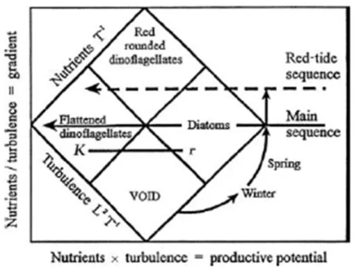
(20) Thèse de Stéphane Karasiewicz, Lille 1, 2017. Chapter 1 – General introduction nitrogen-fixing cyanobacteria, as nitrogen availability relative to phosphorus decreases [Sommer et al., 1986; Sommer, 1989]. The temporal composition of the phytoplankton community depends on the performance of species [Winder and Sommer, 2012]. Marine phytoplankton species numbers are currently estimated to be between 4000 and 5000 [Sournia et al., 1991; Tett and Walne, 1995], but species are still being discovered. It is estimated that 6800 species exist for the diatoms and dinoflagelate alone [Falkowski and Raven, 2007]. The high number of species reflects the high number of different survival strategies of phytoplankton in an unstable and turbulent environment (Table 4.3).. Figure 1.2: Margalef’s (1979) diagram representing the seasonal change phytoplankton community composition as a function of turbulence and nutrients. L and T are standard dimensionless units of lenght and time.. Phytoplankton species performance is mostly influenced by the water column thermal stratification’s impact on vertical mixing, which alters the position of phytoplankton relative to nutrients and light [Winder and Sommer, 2012]. Margalef [1978] proposed an empirical relationship between turbulence, nutrient supply, and taxonomic composition (Figure 1.2). From the model, Margalef defined specific phylogenetic morphotypes (r versus K growth strategists) which can be positioned along a continuum of habitat mixing and nutrient conditions [Margalef, 1978]. r strategies corresponds to species with rapid reproduction when the conditions are turbulent, nutrient concentration are © 2017 Tous droits réservés.. 4. lilliad.univ-lille.fr.

(21) Thèse de Stéphane Karasiewicz, Lille 1, 2017. 1.1. Generalities on phytoplankton ecology. high, such as the diatoms. K strategy are the species with slow reproduction and have a preference for stable habitat conditions, as the dinoflagelates (Figure 1.2). The combination of mixing and nutrient impact the temporal distribution of species during an annual seasonal cycle. Margalef went even further by separating the prediction of species composition under low turbulence conditions: dinoflagellates will dominate under eutrophic conditions (high nutrient concnetrations) and coccolithophore under oligotrophic conditions (low nutrient conditions) (Figure 1.2).. Figure 1.3: Annual selectivity of C, S and R strategy trajectory of the phytoplankton, defined by temperate seasonal variability from Reynolds (2006). In addition to Margalef’s model, Reynolds [2006] developed another model to classify phytoplanktonic species life strategies, based on their respective morphology and physiological traits. The author separated the phytoplankton strategies into three categories: i) colonialist-invasive species (C), ii) stress tolerant species (S) and iii) ruderal species (R) (Figure 1.3). The species using C strategies are characterized by small cell size with a high surface to volume ratio (S/V ), low sedimentation rates but highly exposed to predation. The species with S strategies have a low S/V ratio and are flourishing when the water column mixing is weak, and when the vertical gradient of nutrient and light availability is well established. These conditions are well exploited by species capable of using alternative ways of nutrient acquisitions, such as through nitrogen-fixing, predation and vertical migration. Finally, the R species are generally large elongated cell organisms with a large S/V ratio (Figure 1.3). © 2017 Tous droits réservés.. 5. lilliad.univ-lille.fr.

(22) Thèse de Stéphane Karasiewicz, Lille 1, 2017. Chapter 1 – General introduction These species have a preference for turbulent waters with high nutrient concentrations. The CSR scheme was first developed on terrestrial plants and later adapted to phytoplankton for which the spatial and temporal distribution seemed to be highly correlated to the CSR life strategies [Reynolds, 2006] (Figure 1.3). Despite a well-known seasonal pattern of phytoplankton, the temporal response of the phytoplankton community to the ever changing climatic system is highly variable. The climate system affects phytoplankton fluctuations through many processes, at many time scales in addition to the annual cycle. Therefore understanding the response of the phytoplanktonic community to the changing climate is crucial as it can potentially have severe repercussions on the ecosystem functioning and food-web.. 1.2. Global change. The growth of human population goes in line with the increasing production of food which had altered biogeochemical cycles of nitrogen (N), phosphorus (P), carbon (C) and silica [Seitzinger et al., 2010]. The rate of biologically available nitrogen entering the terrestrial biosphere has doubled in the past decades because human activities via fertilizer production and use, fossil fuel combustion, and cultivation of leguminous crops [Galloway et al., 2004]. The increasing P inputs into the environment has also doubled due to increasing waste water from plant treatments, mining, use of rock phosphate as fertilizer, detergent additives, animal feed supplement and other technical uses [Bouwman et al., 2005; Bennett et al., 2001; Mackenzie et al., 1998]. The major part of N and P is recycled through the terrestrial biosphere but still a significant fraction enter groundwater and surface water, transported by rivers to coastal marine systems [Galloway and Cowling, 2002; Seitzinger et al., 2010]. In combination with the anthropogenic impacts on ecosystems, the Earth’s climate has warmed, during the last century, by approximately 0.6 ◦ C, which was unprecedented compared to the past millennia [McKibben, 2007]. More alarming the rate of warming is expected to increase in centuries to come. Additionally, it has been recognized that the large temporal and spatial variability in the Earth’s climate was due to the atmosphere-ocean system [Stenseth et al., 2003]. Local climatic conditions are greatly influenced by the interannual, subdecadal fluctuations within large-scale climate oscillations [Mantua and Hare, 2002; Stenseth et al., 2003]. Long-term climate change and large-scale climate fluctuations are a crucial attribute of global change, and a wide range of studies have shown links between fluctuations in climate and ecological processes © 2017 Tous droits réservés.. 6. lilliad.univ-lille.fr.

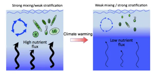
(23) Thèse de Stéphane Karasiewicz, Lille 1, 2017. 1.2. Global change. that affect phytoplankton dynamics [Behrenfeld et al., 2006; Paerl and Huisman, 2008]. Phytoplankton dynamics are linked to the annual fluctuations of temperature, water column stratification, light availability [Sommer et al., 1986; Cloern, 1996]. Climatic change affect these environmental factors and alter phytoplankton community structure and composition. Phytoplankton response can be physiological and/or mediated through effects on environmental factors limiting primary production, most notably light and nutrients [Winder and Sommer, 2012].. 1.2.1. Temperature effects on phytoplankton. Figure 1.4: Warming effect on the water stratification (blue arrows), in association with nutrient mixing (black arrows), phytoplankton production and cell size Winder et al. (2012).. Plant metabolism, photosynthesis and respiration, are directly affected by temperature but primary producers metabolic rates are mostly limited by the former rather than the latter [Dewar et al., 1999]. Phytoplankton can bloom on sea ice margins [Smith and Nelson, 1985] and under clear ice in lakes [Vehmaa and Salonen, 2009] revealing tolerance of some species which still flourish under conditions of low temperature. Light-limited photosynthetic rates are therefore less sensitive to temperature. Oppositely, light saturation can potentially occur as light-saturated rates increase with temperature and light availability [Tilzer et al., 1986]. With global warming, an increasing production of light-saturated rates photoautotrohic will go along with a decline of the light-limited ones [Winder and Sommer, 2012]. Warming should lead to rising plant growth rates © 2017 Tous droits réservés.. 7. lilliad.univ-lille.fr.

(24) Thèse de Stéphane Karasiewicz, Lille 1, 2017. Chapter 1 – General introduction and increase biomass with sufficient resource supply [Padilla-Gamino and Carpenter, 2007]. However, the heterotrophic organisms’ respiratory metabolism is more sensitive to temperature [Allen et al., 2005; López-Urrutia et al., 2006]. Therefore global warming should increase herbivory more strongly than primary production and potentially should increase the top-down control with rising grazing rates [O’Connor et al., 2009; Sommer et al., 2011]. The increase grazing pressure should affect phytoplankton’s production and taxonomic composition [Winder and Sommer, 2012]. Phytoplankton community composition would most likely be affected by the thermal stratification of the water column which can extend the growing season and vertical mixing processes [Schindler et al., 1996; Rodriguez et al., 2001; Diehl et al., 2002; Smol et al., 2005] (Figure 1.4). As previously mentioned, mixing is a key factor for phytoplankton growth as it affects resource acquisition, nutrient and light of individual species [Diehl et al., 2002; Salmaso, 2005]. Heat exchange stratifies the water column and inhibit mixing, while wind action creates turbulent kinetic energy enhancing the mixing [Wetzel, 2001] (Figure 1.4). The two opposite factors structure the seasonal cycle: summer stratification versus winter mixing. The balance between these two states of stratification will also be affected by global warming [King et al., 1997; Boyd and Doney, 2002; Livingstone, 2003]. The variability in thermal stratification magnitude will directly affect turbulence along with the sinking velocity of phytoplankton community [Livingstone, 2003; Huisman et al., 2006]. It will favor smaller, buoyant species which willl have a competitive advantage over the larger sinking species which will not have as many opportunities to resuspend [Findlay et al., 2001; Huisman et al., 2004; Strecker et al., 2004]. Water column mixing affects nutrient available for phytoplankton. Nutrient-depleted conditions in surface waters is enhanced by stratification which decreases the upward flux of nutrients from deep-water [Livingstone, 2003; O’Reilly et al., 2003; Schmittner, 2005]. Altering mixing regimes affects the competitive advantage of specific phytoplankton morphology, that are better competitors for nutrients [Falkowski and Raven, 2007] and more buoyant at the surface water, such as cyanobacteria [Huisman et al., 2004]. In association with climate change, the increasing nutrient concentration can be related to anoxic conditions [Wilhelm and Adrian, 2008], resulting to similar condition than the processes eutrophication. Moreover, the frequency of extreme rainfall and severe drought has increased since 1970s [McKibben, 2007; Stocker, 2014], increasing terrestrial nutrient runoff [Briceño and Boyer, 2010].. © 2017 Tous droits réservés.. 8. lilliad.univ-lille.fr.

(25) Thèse de Stéphane Karasiewicz, Lille 1, 2017. 1.2. Global change. Figure 1.5: Glibert et al. 2017 scheme showing the effect of eutrophication with increasing N and P loading on biodiversity and biogeochemistry. The lower panel illustrates the effect of increasing imbalance between N and P.. 1.2.2. Eutrophication. The increasing runoff modifies the resource ratio of the ecosystems, depending on the catchment geochemistry modifying the competitive advantage of phytoplankton species [Winder and Sommer, 2012] (Figure 1.5). The impact of increasing N export of rivers into estuarine, coastal, and marine ecosystems depends on phosphorous (P) and silicon (Si) availability. N and P limit phytoplankton growth, in general, and Si limits diatoms’ growth in particular [Rabalais, 2002] (Figure 1.5). The eutrophication process is a biogeochemical enrichment response of plants to nutrients, often to nitrogen (N), and phosphorous (P) increase [Bouwman et al., 2005]. In aquatic systems, the consequences of eutrophication is correlated with an increasing primary production and respiration [Bouwman et al., 2005] (Figure 1.5). Eutrophication has advanced, worldwide, in all densely populated countries, and it is affecting lakes, reservoirs, estuaries, and coastal seas [Vollenweider, 1992]. During the past decades, whilst the flux N and P are increasing [Smith et al., 2003], the loads of Si remained constant and even decreased in rivers where dams were built [Conley, 2002]. Consequently, it altered the stoichiometric balance of N, P, and Si [Rabalais, 2002], consequently impacting the primary production in coastal marine systems, quantitatively and qualitatively. Species, other than diatoms become competitively superior and become dominant, such as flagellated algae which including noxious bloom-forming communities [Turner et al., © 2017 Tous droits réservés.. 9. lilliad.univ-lille.fr.

(26) Thèse de Stéphane Karasiewicz, Lille 1, 2017. Chapter 1 – General introduction 2003]. Therefore the food web dynamics leading to fisheries harvests are affected by shifts in the relative availability of N, P, and Si [Bouwman et al., 2005]. For coastal regions, enhanced upwelling with increasing temperature are expected to increase the availability of nutrients and stimulate phytoplankton production [Rabalais, 2002] but changes in the amount, form (dissolved inorganic, organic, particulate), and ratios will contribute to numerous negative human health and environmental impacts [Seitzinger et al., 2010]. Along with eutrophication, a loss of habitat and biodiversity, hypoxia and fish kills are expected with increasing harmful algae bloom (HAB) [Billen et al., 2007; Diaz and Rosenberg, 2008; Howarth et al., 1996; Rabalais, 2002; Turner et al., 2003; Davidson et al., 2012; Heisler et al., 2008].. Figure 1.6: Wells et al. 2015 literature overview of the climate change effet on the different types of HAB. Arrows indicating the trend of the changes and the + indicate the confidence level: (+) reasonably likely and (++) more likely. OA: Oceanic acidification.. © 2017 Tous droits réservés.. 10. lilliad.univ-lille.fr.

(27) Thèse de Stéphane Karasiewicz, Lille 1, 2017. 1.3. Harmful Algae. 1.3 1.3.1. Harmful Algae Generalities. A subset of phytoplankton species may be harmful to human health (e.g. through the production of natural biotoxins), or to the ecosystem service used by humans (e.g. causing mortality of farmed fish and restricting the harvesting of shellfish). They are widely referred to as “Harmful Algae” and the term “Harmful Algal Bloom” (HAB) refers to their occurrence and effect [Davidson et al., 2012]. The phenomena occurs throughout the world’s oceans leading to increasing concerns for human health and environmental preservation [McPartlin et al., 2017]. Additionally, the economic loss associated with HABs was estimated at tens of billions of US dollars annually [Sanseverino et al., 2016]. Two different types of harmful algae exist (Figure 1.6). The first group produces toxins or harmful metabolites, such as toxins linked to wildlife death or human seafood poisonings. The toxins of some phytoplankton species are so potent, even at very low concentrations, it makes their bloom very dangerous. The second group of species are nontoxic but causes harm by being highly productive, creating foams or scums, depleting oxygen as bloom collapses, or the destruction of habitat for fish or shellfish by shading of submerged vegetation [Davidson et al., 2012] (Figure 1.6). Nutrient ratios have been suggested to influence biotoxin producing HAB species magnitude [Fehling et al., 2004; Granéli and Flynn, 2006]. The nutrient ratio hypotheses [Officer and Ryther, 1980; Tilman, 1977] stipulated that perturbation in the nutrient supply ratio will result in the environmental selection of potentially harmful species [Smayda, 1990; Heisler et al., 2008]. The perturbation in the nutrient ratio is thought to be anthropogenically induced [Falkowski, 2000; Conley et al., 2009], and the changes in N:P ratio seemed as a possible mechanism for HABs. The nutrient form may also be important. Phytoplankton has a preference, for uptake of a more reduced form of N, such NH4 + [Dortch, 1990; Flynn et al., 1993; Rees et al., 1995] which can be produced by the food web [Davidson et al., 2005], or have natural and anthropogenic origins [Eppley et al., 1979]. The availability of the natural and anthropogenic dissolved organic nutrients (i.e . runoff of nitrogenous nutrient urea and fertilizer), has also been suggested to have a significant impact on HABs [Antia et al., 1991; Carlsson et al., 1993; Bronk, 2002; Lønborg et al., 2009]. But in reality the response of HAB to the climate change and eutrophication are highly speculative [Wells et al., 2015] (Figure 1.6). Fundamental changes in HAB research strategies is necessary to meet the complex ecological and multi-environmental stresses that shape phytoplankton communities [Wells et al., 2015]. Two key challenges are needed to © 2017 Tous droits réservés.. 11. lilliad.univ-lille.fr.

(28) Thèse de Stéphane Karasiewicz, Lille 1, 2017. Chapter 1 – General introduction move forward in HAB research. First, to obtain evidence that global change can cause alterations in HAB distribution, prevalence or character (Figure 1.6). And second, to develop a scenario with empirical evidences on the causal effect of the environmental and ecological factors which can impact the range of expansion or contraction, and emergence of new patterns for HAB.. Figure 1.7: Left: a microscopic view of Phaeocystis globosa colony. Right: Foam accumulation produced by the degradation of the colonies. 1.3.2. An invasive species: Phaeocystis spp.. The marine prymnesiophyte Phaeocystis genus is a common species of the winter-spring phytoplankton community in north-temperate coastal seas [Cadée and Hegeman, 2002; Schoemann et al., 2005]. Phaeocystis’ is capable of forming high monospecific blooms of gelatinous colonies (>10 mg.C.L-1 ; up to 200×106 cells.L-1 ) [Schoemann et al., 2005] which endorses a substantial amount of resources from the ecosystem, altering trophic pathways [Tang et al., 2001] (Figure 1.7). Consequently Phaeocystis is considered to be one of the few “keystone” phytoplankton species whose blooms can significantly alter the functioning of an ecosystem [Lancelot et al., 1994; Verity and Smetacek, 1996; Verity et al., 2007] by modifying the biogeochemical cycling [Smith Jr et al., 1991; Stefels et al., 1995] and the food web structure [Rousseau et al., 2000]. The variability of Phaeocystis high abundance occurrence from year to year is still not well understood. The “silicate-Phaeocystis hypothesis”, suggesting that diatoms outgrow Phaeocystis until silicate becomes limiting was first proposed as an explanations for Phaeocystis bloom variability [Lancelot et al., 1987; Reid et al., 1990]. Since, other researches had shown that low silicate © 2017 Tous droits réservés.. 12. lilliad.univ-lille.fr.

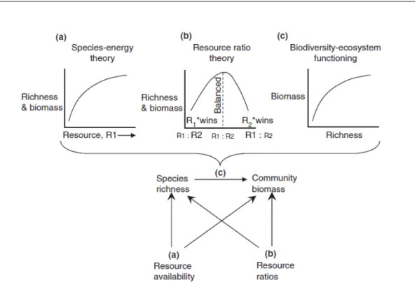
(29) Thèse de Stéphane Karasiewicz, Lille 1, 2017. 1.4. Link between diversity and productivity. concentration is not the only condition. Peperzak et al. [1998] and Peperzak [2002] showed that diatoms can be out-competed by Phaeocystis globosa under high light availability. Phaeocystis annual bloom regulation seemed to be multifactorial involving variation in both long-term climate trends [Cadée and Hegeman, 1986, 2002] and the influence of anthropogenic activity on nutrient concentration [Riegman and Noordeloos, 1992; Cadée and Hegeman, 2002; Tungaraza et al., 2003; Gypens et al., 2007; Lancelot et al., 2007; Breton et al., 2006] and nutrient ratios [Lancelot et al., 1987]. Ecosystems which are dominated by Phaeocystis are often related with commercially important stocks of crustaceans, mollusks, fishes and mammals. Phaeocystis potential impact on higher-trophic levels makes it a threat to human activities, such as fisheries, aquaculture, and tourism via odorous foams on beaches during the bloom’s wane [Lancelot et al., 1987] (Figure 1.7). During period of high abundance, the blooms have been reported to cause net-clogging [Savage, 1930], fish mortality [Savage [1930]; Hurley [1982]; Rogers and Lockwood [1990]; Huang1999] and altering fish taste along with a decrease in shell fish growth and reproduction [Levasseur et al., 1994; Pieters et al., 1980; Davidson and Marchant, 1992; Prins et al., 1994; Smaal and Twisk, 1997]. Additionally, toxins have been collected from Phaeocystis [He et al., 1999; Stabell et al., 1999; Hansen et al., 2003]. Obtaining evidence of Phaeocystis response to global change and its impact on the local biodiversity and ecosystem functioning is crucial due to its high HAB potential. Furthermore, understanding the causal link between, the HAB, biodiversity and the global change will shed light on its capacity range expansion or contraction, and emergence of new phytoplankton communities.. 1.4. Link between diversity and productivity. One of the oldest questions in biology is how resource, species diversity and productivity are related. Historically, it was long thought that productivity drives diversity, creating the common relationship where diversity is highest at intermediate levels of productivity [Currie, 1991, Rosenzweig and Abramsky [1993]]. Theories explaining the causalities between resources and communities’ diversity include the Species-Energy Theory (SET) [Wright, 1983] and the Resource-Ratio Theory (RRT) [Tilman, 1982]. SET hypothesis that the variation in species richness can be explained by the available energy which also controls, population sizes and stochastic extinction’s probability [Wright, 1983] (Figure 1.8). The quantity of available energy is measurable in units of energy per time (e.g. joules per year). RRT stipulates that species richness is determined by the resources supply imbalance which increases the © 2017 Tous droits réservés.. 13. lilliad.univ-lille.fr.

(30) Thèse de Stéphane Karasiewicz, Lille 1, 2017. Chapter 1 – General introduction. Figure 1.8: Cardinale et al. 2009 Multivariate Productivity-Diversity (MPD) model regrouping three theories, (a) Species-energy theory, (b) Resource ratio theory and (c) Biodiversity-ecosystem functioning. competitive possibilities for replacements [Tilman, 1982] (Figure 1.8). More recently, researchers have tackled the problem from a different angle, viewing species diversity as a driver of productivity [Chapin et al., 2000; Tilman, 2000; Fridley, 2001; Loreau et al., 2002; Naeem, 2002; Hooper et al., 2005] the “biodiversity-ecosystem functioning” (BEF) theory [Naeem et al., 1994; Gross and Cardinale, 2007; Hillebrand and Matthiessen, 2009] (Figure 1.8). The paradigm elaborates connections between our distinct variables: (1) the amount of available resources, (2) the resources’ stoichiometric ratios, (3) the produced biomass by the studied community, and (4) the diversity of cooccurring species in the community [Cardinale et al., 2009b] (Figure 1.8). The biodiversity-productivity relationship is constrained by the resource supply rates and ratios making ecosystem stoichiometry (ES) an essential component in the biodiversity and productivity relationship [Hillebrand and Lehmpfuhl, 2011]. This contemporary view on productivity-diversity relationships has often been studied in the anthropological context when biodiversity decreases due to human impact on natural systems, such as eutrophication, causing an imbalance resource ratio and a reduction of productivity [Cardinale et al., 2009b; Hillebrand and Lehmpfuhl, 2011; Gross and Cardinale, 2007]. Since, © 2017 Tous droits réservés.. 14. lilliad.univ-lille.fr.

(31) Thèse de Stéphane Karasiewicz, Lille 1, 2017. 1.4. Link between diversity and productivity. the theory had been mostly applied on terrestrial ecosystem and on freshwater ecosystems. Marine diversity-productivity relationship still remains to be studied. Only recently, meta-analyses and experiments have shown the effect of the resources availability and ratios onto the diversity-productivity within the phytoplankton community [Lewandowska et al., 2016; Lehtinen et al., 2017; Hodapp et al., 2015]. Small-scale experimentation with artificially assembled microbial communities have been increasingly applied to diversity-productivity studies, especially in aquatic environments [Striebel et al., 2009; Gamfeldt and Hillebrand, 2011]. Under the current global changes the phytoplankton community will be impacted by the changing climatic conditions, affecting the annual, and the long-term diversity-productivity relationship. Furthermore, the possible increasing HAB occurrence could have an additional effect on the diversity-productivity relationship. Phytoplankton having such an pivotal role in the marine ecosystem and ecosystem functioning, the understanding of the response in diversity-productivity relationship is of crucial importance.. Figure 1.9: Figure inspired from Jackson S, Overpeck JT. (2000). The environmental gradients, E1 and E2 , define the realized environmental space E. The fundamental niche, Nf , intersect E, creating the existing fundamental niche, Np . The realized niche, NR is therefore included into Np but it further restricted by the biotic interaction, B.. © 2017 Tous droits réservés.. 15. lilliad.univ-lille.fr.

(32) Thèse de Stéphane Karasiewicz, Lille 1, 2017. Chapter 1 – General introduction. 1.5. Niche concept. Ecological niche is a pivotal theory to understand how the changing environment affects species abundance patterns. J. Grinnell and C. Elton first developed the idea in the early 20th century, an idea which was latter brought back by G. E. Hutchinson and R. MacArthur during the 1950s’ and 60s’. Under ongoing global changes, the niche concept has regained interest as it has the potential to predict the future of living species [Peterson et al., 1999; Chase and Leibold, 2003; Wiens et al., 2009]. There are three different niche perspectives focusing on different aspects of the niche concept. First, the Grinnellian niche concept in which, the niche is considered to be included in the environmental space that a species can occupy and is defined by abiotic factors [Wiens et al., 2009]. The Eltonian niche focuses on the species or group of species’ functional role in the ecosystem [Polechová and Storch, 2008; Wiens et al., 2009]. Finally, Hutchinson [1957] niche concept is a n-dimensional conceptual space, defined by environmental factors that influences fitness of individuals of a species. Two types of niches were defined. The fundamental niche is described as the n-dimensional hypervolume, restricted by multiple resources and environmental factors, where a species can live indefinitely, in the absence of biotic interactions [Hutchinson, 1957]. The realized niche is described as a subset of the fundamental niche that is constrained by additional biotic interactions (e.g., competition, predation, mutualism, dispersal, and colonization). Despite being an attractive concept, the applicability of the concept onto the real world is questionable. As Griesemer [1992] reported, Hutchinson’s niche concept is static and does not consider temporal environmental changes and the variability of the species response. Environmental change creates different combinations of niche variables and could be challenging to identify the relevant factors leading to the species persistence through time [Jackson and Overpeck, 2000]. Therefore, the finite combinations of n-environmental factors relevant to a species exist at any given time and the environmental conditions which actually occurs at a time t is called the realized environmental space, E (Figure 1.9). The intersection between the realized environmental space and the fundamental niche, Nf , is named the existing fundamental niche, Np (Figure 1.9) [Soberón and Nakamura, 2009; Peterson, 2011a]. The realized environmental space should change with global changes and the realized niche, NR , of any given species of a community should also vary. Therefore the biotic interaction, B, between species will also be subjected to change (Figure 1.9). The omission of biotic interactions in niche research is a major setback for measuring accurate niches [Davis et al., 1998; Soberón and Nakamura, 2009] © 2017 Tous droits réservés.. 16. lilliad.univ-lille.fr.

(33) Thèse de Stéphane Karasiewicz, Lille 1, 2017. 1.6. Problematic. and its temporal variability and affect onto the species community is essential for understanding the fate of phytoplankton along with HAB.. 1.6. Problematic. Phytoplankton annual cycle will most likely be affected by global warming. For the most pessimistic scenario, the climatic model predict an increase of 4◦ C for the sea surface temperature. Human activity is expected to rise along with their respective nutrient input, especially N and P, disturbing the N:P ratio within the aquatic ecosystem. The concomitant changes will affect the phytoplanktonic community composition, diversity, and consequently, the primary production impacting the rest of the food web like some other ecological functions. The study of the modification caused by these disturbances on the phytoplanktonic composition is a necessity due to their key role in the ecosystem functioning. A relative small number of studies have investigated the simultaneous effect of several environmental variables on the phytoplankton response and effect on productivity. Despite this limitation, it was revealed that the phytoplankton growth and life strategies would be modified and this will have as a consequence the appearance of harmful algae species. It was reported that the diversity and productivity is expected to increase and to decrease respectively during the bloom of an invasive species [Sax and Gaines, 2003; Byrnes et al., 2007]. The harmful algae blooms are suggested to be increasing with further anthropogenic eutrophication and warming. In reality, the hypothesis remain highly speculative as environmental multifactorial studies on HAB are still lacking. The development of a new method is required to prevent and predict the occurrence of HAB. In combination with global change, the response of phytoplankton community, composition and succession, under conditions of HAB and non-HAB remains to be revealed. The diversity-productivity relationship in phytoplankton community has already been reported, but mostly in small time scale experimental condition and more rarely in situ. Furthermore, its study in marine ecosystem is still in its infancy and awaits to be developed. The marine phytoplankton diversity-productivity relationship, in association with global change and the invasive species, is still unknown but it is expected to differ on an annual, and from a year-to-year basis. The Hutchinson’s niche concept has regained interest to study species’ response to global changes and invasive species studies. Researchers on species’ niche acknowledge the biotic interaction as a limitation, and its potential dynamic effect on realized niche under changing climatic conditions, but it persists to be neglected. The actual theory suggests that the fundamental niche is needed to estimate the biotic in© 2017 Tous droits réservés.. 17. lilliad.univ-lille.fr.

(34) Thèse de Stéphane Karasiewicz, Lille 1, 2017. Chapter 1 – General introduction teraction effect onto the species’ realized niche. Unlike the realized niche which can be measured, the fundamental niche cannot be observed in nature, and requires extensive calculation and modelling. The actual niche concept could be revised for greater application to investigate the species niche response under temporal, spatial and/or episodical scale and with biological interaction taken into account explicitly. This is of special importance for phytoplankton to study to so-called Hutchinson’s “plankton paradox”. The thesis aim was to describe and to measure the temporal responses and causalities of the phytoplankton community structure, with the occurrence of a harmful algae, under global changes. The investigation will be divided into three sections and related questions: 1. Can a niche concept and a statistical method be developed to allow the observation and quantification of the species’ niche response to global changes? Can the biotic interaction affecting the species’ niche be observed and quantified? 2. What is the response of the phytoplankton community structure under HAB or no HAB conditions? What environmental conditions explain the occurrence of a harmful algae? 3. How global change and the invasive species affect the diversity-productivity relationship in a short-term and long-term scales?. © 2017 Tous droits réservés.. 18. lilliad.univ-lille.fr.

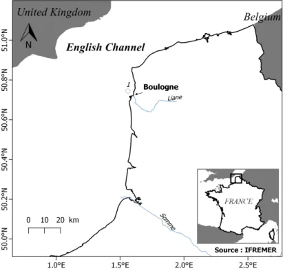
(35) Thèse de Stéphane Karasiewicz, Lille 1, 2017. Chapter 2. Materials and Methods. 2.1. Data. Since 1984, IFREMER (Institut Français de Recherche et d’Exploitation de la Mer) have established an observation and monitoring network for marine phytoplankton, the REPHY (Réseau d’Observation et de Surveillance du Phytoplancton Marin). The network was created to answer two complementary objectives: • An environmental heritage objective for the sake of acknowledging the biomass, abundance and the composition of marine phytoplankton in coastal and lagoonal waters, in order to describe the spatial-temporal dynamic of the different phytoplanktonic species. Through this objective, the REPHY also aims to establish an inventory of exceptional blooms, as such as the colored waters. • A health monitoring objective, in order to detect and follow the development of toxin producing species, which accumulates in sea product destined for human consumption and represents a potential health issue. It is completed by toxin research in bivalve mollusk present in production area or in natural stocks. Within the REPHY framework, three phytoplankton observation strategies are in place. They are mentioned in the REPHY’s Protocole Chart 2012-2013 [Belin and Neaud-Masson, 2012]. Only the “Total Phytoplankton” strategy, from which the data were used for the analysis, are briefly reported bellow: “Total Phytoplankton” strategy is concerned by regularly covering locations to report and count all recognizable phytoplankton species present in a sample,under an optical microscope. It provides the essential time series required for phytoplanktonic community studies. The acquisition frequency of the data, so called “Total Flora” is monthly to bimonthly basis depending on the location. For all monitoring locations, the REPHY applies a standardize protocol for sampling, observation, counting of the phytoplankton along with environmental parameter measurements. © 2017 Tous droits réservés.. 19. lilliad.univ-lille.fr.

(36) Thèse de Stéphane Karasiewicz, Lille 1, 2017. Chapter 2 – Materials and Methods. Figure 2.10: Location of station where data is collected along the coast of France.. The species biovolume were collected from the Olenina et al. [2006] study, and if the species’ biovolume was not reported in the the article, the biovolume was searched on http://eol.org/traitbank by using the R packages ”Reol” and ”traits” [Banbury and O’Meara, 2014; Chamberlain et al., 2016].. 2.2. Community analysis. The phytoplankton species do not equally contribute to the community abundance. A set of species combination which contribute the most into the community abundance pattern is required to reveal the most important species. The search for the best combination of species possible was done with the BVstep analysis [Clarke and Warwick, 2001]. The analysis requires two matrices, the faunal matrix (fixed matrix) and its transposed version, from which the similarity matrix (Bray-Curtis distance) are calculated [Clarke and Warwick, 2001]. The idea is to find the smallest possible species combination, from the transposed matrix, that matches as near as possible the full species set from the fixed matrix. The Bray-Curtis similarity matrix for the smallest species subset has to be at least correlated at ρ = 0.95 with the fixed matrix. The analysis © 2017 Tous droits réservés.. 20. lilliad.univ-lille.fr.

(37) Thèse de Stéphane Karasiewicz, Lille 1, 2017. 2.3. Niche analysis. uses the step-wise procedure, which subsequently operates and includes the both forward and backward-stepping phases. The procedure starts with a null set, choosing the species which best maximizes ρ, then adds a second and a third species to improve ρ. The backward elimination now starts and checks if the first selected species can be dropped. In other words, if the second and third species alone have a greater ρ than with the three species together. The algorithm continues, with each step selecting the best species to add (forward phase) or to drop (backward phase) from the existing combination. The procedure goes on until no further improvements are possible by the addition of a species to the existing combination of species [Clarke and Warwick, 2001].. 2.3. Niche analysis. Since Hutchinson [1957] niche concept, authors promoted different measurements for niche separation and niche breadth [Hurlbert, 1978; Colwell and Futuyma, 1971; Feinsinger et al., 1981]. In community studies, the term niche refers the preferential habitat for species [Braak and Verdonschot, 1995]. The selection of the appropriate ordination technique in terms of species response models and weighting options depends mainly on the objectives. Herein, the aim is to understand how species respond to environmental gradients. Among other method, the Outlying Mean Index (OMI) is a multivariate statistical analysis which separates community species niches and measures the distance between the mean habitat conditions used by each species and the mean habitat conditions of the study area [Dolédec et al., 2000; Thuiller et al., 2004]. Unlike other methods, the OMI makes no assumption about the shape of species response curves to the environment (e.g. unimodal or linear). Furthermore, OMI analysis gives equal weight to species-rich and species-poor sites, which is not the case for the canonical correspondence analysis (CCA) and redundancy analysis (RDA). The OMI analysis gives the mean position of the species in the environmental space (along each environmental axis), which represents a measure of the distance between the mean habitat conditions used by the species and the mean habitat conditions of the study area. It measures the species susceptibility to select a specialized environment. The OMI analysis calculates the species niche of the community over the entire data set, meaning that it comprises all sampling dates (or sites). Therefore, in order to extract events or specific time scale, the analysis needs to be divided into subsets. The OMI analysis, being a two table ordination method (species table Y responding to the environmental table Z), both tables have to be decomposed. In addition, the species’ mean position, at a time t, should be calculated from the mean © 2017 Tous droits réservés.. 21. lilliad.univ-lille.fr.

(38) Thèse de Stéphane Karasiewicz, Lille 1, 2017. Chapter 2 – Materials and Methods environmental habitat condition and, from the mean environmental habitat condition at time t.. 2.3.1. Species frequency table. Here and elsewhere, we follow the mathematical notations used by [Dolédec et al., 2000]. Let us extract YK (k samples×t species), from the faunistic table Y(n samples × t species) with 1 ≤ k ≤ n. Let us transform subset YK into a species profile table (noted FrK ) that contains the frequency of species for each SUs, fKis /j as follows: fKis /j =. yKis j yK.j. 1 ≤ is ≤ k, 1 ≤ j ≤ t. (2.1). where yKis j is the abundance of species j in SU is and yK.j the column total of species j equal to yK.j =. k X. yKis j. (2.2). is =1. Then the species profile table Fr∗ concatenates FrK as follows: . .  Fr1   .   .. . Fr∗ =.     Fr   K  .   .   .   . 1≤K≤N. (2.3). FrN. with N the number of subsets. Inspired by the OMI analysis [Dolédec et al., 2000] and the decom position of marginalities used in K-select analysis [Calenge et al., 2005], we propose to calculate two additional marginalities. First, the Within Outlying Mean Index to G (WitOMIG) is the species marginality (i.e., the weighted average of sampling units of a given subset used by the species) to the average habitat conditions of the sampling domain (G; see Eq. 2.7 in the followed section). Second, the Within Outlying Mean Index to GK (WitOMIGK ) is the species marginality compared to the average habitat condition used by the community in a K subset habitat conditions (GK ; see Eq. 2.16 in the followed section) © 2017 Tous droits réservés.. 22. lilliad.univ-lille.fr.

(39) Thèse de Stéphane Karasiewicz, Lille 1, 2017. 2.3. Niche analysis. 2.3.2. Subniche parameters calculated from the origin G. The center of gravity (G) of SUs is at the origin of the axes of the OMI analysis and corresponds to the overall mean habitat conditions used by the taxa in the assemblage [Dolédec et al., 2000]. Let us consider N subsets habitat conditions of the environmental table Z0 equals to: . .  .  .  Z1   .   ..   Z0 =  ZK  1 ≤ K ≤ N  .   .   .  . ZN. (2.4). . Let us extract ZK (k × p), a matrix of Z0 (n × p), having k rows, with 1 ≤ is ≤ k and p variables (Figure 3). Let the faunistic frequency table, FrK (k × t) contains the frequency of t species in the k SUs. Mi represents SU i of table Z0 in the multidimensional space Rp . Let consider MKis , representing SU is of table ZK in the same multidimensional space Rp . The total inertia of table ZK equals: ITK (j) =. k X. fKis /j k MKis k2Ip. (2.5). is =1. The inertia ITK (j) represents the total inertia of ZK weighted by the species j profile. Similarly to the proposal of Dolédec et al. [2000], the SUs is that do not have species j do not add to the species j inertia. Let consider a Ip -normed vector uK (k uK k2Ip = 1). The projection of the k rows of the matrix ZK onto the vector uK results in a vector of coordinates ZK uK . Therefore, the average position of species j on uK , equivalent to the center of gravity of species j, is defined as: TKj = f> K ZK uK. f> K = (fK1/j , . . . , fKis /j , . . . , fKk/j ).. (2.6). With Eq. S8, marginality within a subset of habitat conditions, or withinsubset outlying mean index (WitOMIG) of species j {[}noted maK (j){]} along uK equals: 2 maK (j) = TK2 j = (fK | ZK uK )2Ip = (Z> (2.7) K uK | f)Ip © 2017 Tous droits réservés.. 23. lilliad.univ-lille.fr.

(40) Thèse de Stéphane Karasiewicz, Lille 1, 2017. Chapter 2 – Materials and Methods. This marginality represents the deviation between the average position of species j within subset K from the origin (G). Also equivalent to the distance between the subset average habitat conditions used by species (j) and the overall average habitat conditions found in the area (G). From Eq. 2.7, the maximization of maK (j) has for solution uK equal to: uKj =. Z> K fK . > k Z K f K kI p. (2.8). Vector uKj , defined the direction of the species j, within the subsets (marginality axis of species j within subset K), for which the average position of species j within subset K is as far as possible from the overall average habitat conditions (G). In addition, the dispersion or tolerance [noted TmK (j)]of SUs is which contains species j, can be calculated. Let mKis be the projection of MKis , onto the marginality axis, as follows: TmK (j) =. k X. fKis /j k GKj − mKis k2Ip. (2.9). is =1. TmK (j) represents the subniche breadth of species j under the habitat conditions defined by ZK . Finally, similarly to the proposal of Dolédec et al. [2000], the projection of the SUs of subset K onto the plane orthogonal to the marginality axis returns a residual tolerance {[}noted TrK (j){]} and the decomposition of the species j total inertia under the subset habitat conditions can be written as follows: ITK (j) = maK (j) + TmK (j) + TrK (j). (2.10). The niche variability of the species j thus comprises of the three components advocated by Dolédec et al. [2000]: (1) an index of marginality or WitOMIG, i.e., the average distance of species j within subsets to the uniform distribution found in the sampling domain (G); (2) an index of tolerance or subniche breadth and (3) a residual tolerance, i.e., an index that helps to determine the reliability of the subset habitat conditions for the definition of the subniche of species j. © 2017 Tous droits réservés.. 24. lilliad.univ-lille.fr.

(41) Thèse de Stéphane Karasiewicz, Lille 1, 2017. 2.3. Niche analysis. Furthermore the total species inertia IT (j) calculated in Dolédec et al. [2000], can be recalculated using the inertia of species ITK (j) as follows: IT (j) =. v u N uX t (I. TK (j). K=1. ×. yK.j 2 ) y.j. (2.11). where y.j corresponds to the total species j abundance in the faunistic table Y.. 2.3.3. Subniche parameters calculated from a sub-origin GK. In the previous section, the subniche parameters are estimated considering the average habitat conditions (G) used by the all species in the assemblage. The subniche parameters can also use the average subset habitat conditions (GK ) and the corresponding subsets of species. Let us consider again the matrices ZK , which are centered using their respective mean to yield ZK ∗ , thus making the global table Z∗ : . .  .  . ∗  Z1   .   .. .  Z∗ =  ZK ∗   .   .   .  . ZN ∗. (2.12). . Let us consider again the faunistic table, FrK (k × t) that contains the species frequency (Figure 3). The equations are the same as previously but considering the N centered subset habitat conditions ZK ∗ (Details in the Appendix S1). We obtain similarly the total inertia of ZK ∗ , ITK ∗ , and the inertia of species j, ITK ∗ (j), can be decomposed into its marginality or WitOMIGK , maK ∗ (j), its tolerance TmK ∗ (j) and its residual tolerance TrK ∗ (j). Let us extract ZK ∗ (k × p), a matrix of Z∗ (n × p) with k rows. Let the faunistic table, FrK (k × t) contain the frequency of t species in the k SUs. Let Mis represent SU is of table ZK ∗ (k × p) in the multidimensional space Rp . Let MKi∗s represent the SU is subset habitat conditions of table ZK ∗ in the same multidimensional space Rp . The total inertia of the matrix ZK ∗ , equals: © 2017 Tous droits réservés.. 25. lilliad.univ-lille.fr.

(42) Thèse de Stéphane Karasiewicz, Lille 1, 2017. Chapter 2 – Materials and Methods. k X. ITK ∗ =. is =1. pKi∗s k MKi∗s k2Ip. (2.13). with pKi∗s being the weight of SU is . The inertia of species j considering the matrix ZK ∗ equals: ITK ∗ (j) =. k X is =1. fKis /j k MKi∗s k2Ip. (2.14). The inertia ITK ∗ (j) represents the inertia weighted by the species profile j. The SUs is that do not have species j do not add to the species j inertia. Let us consider a Ip normed vector uK ∗ (k uK ∗ k2Ip = 1). The projection of the k rows of the matrix ZK ∗ onto the vector uK ∗ results in a vector of coordinates ZK ∗ uK ∗ . Therefore, the average position of species j on uK ∗ , equivalent to the center of gravity of species j within a subset of habitat conditions is defined as: TKj∗ = f> f> (2.15) K ZK ∗ uK ∗ K = (fK1/j , . . . , fKis /j , . . . , fKk/j ).. With the Eq. S19, marginality within a subset of habitat conditions, or within subset outlying mean index to GK (WitOMIGK ) of species j [noted maK ∗ (j)] along uK ∗ equals: 2 maK ∗ (j) = TK2 j∗ = (fK | ZK ∗ uK ∗ )2Ip = (Z> K ∗ uK ∗ | fK )Ip. (2.16). This marginality represents the deviation between the average position of species j within subsets from the subset habitat origin (GK ). Also equivalent to the distance between the average subset habitat conditions used by species j and the average subset habitat conditions of the subset area. From Eq. 2.16, the maximization of maK ∗ (j) as for solution uK ∗ : uKj∗ =. Z> K ∗ fK . > k ZK ∗ fK kIp. (2.17). Vector uK ∗ j , defined the direction of the species j, within the subsets (marginality axis of species j within the subsets), for which the average position of species © 2017 Tous droits réservés.. 26. lilliad.univ-lille.fr.

(43) Thèse de Stéphane Karasiewicz, Lille 1, 2017. 2.4. Structural Equation Modelling. j within subsets is as far as possible from the subset habitat conditions found in the area GK . In addition, the dispersion or tolerance [noted TmK ∗ (j)] of SUs is that contains species j can be calculated. Let mKi∗s be the projection of MKi∗s , onto the marginality axis as follows: TmK ∗ (j) =. k X is =1. fKis /j k GKj − mKi∗s k2Ip. (2.18). TmK ∗ (j) represents the subniche breadth of species j under the subset habitat conditions defined by ZK ∗ . Similarly to the proposal of [Dolédec et al., 2000], the projection of the k SUs of subset K onto the plane orthogonal to the marginality axis returns a residual tolerance [noted TrK ∗ (j)] and the decomposition of the species j total inertia under the subset habitat conditions equals: ITK ∗ (j) = maK ∗ (j) + TmK ∗ (j) + TrK ∗ (j) (2.19). 2.4 2.4.1. Structural Equation Modelling Description and approaches. The Structural Equation Modelling (SEM), or pathways analysis, are multivariate statistical calculations which allow to concurrently analyse a network of variable relationships and considering direct and indirect relationships with error measurements. It is a well adapted method to analyse ecological processes due to their hierarchical structure and patterns [Grace, 2006; Arhonditsis et al., 2006]. For instance, the SEM gives the opportunity to create relationship models between ecological concepts, such as biodiversity and ecosystem productivity, which are often not measured but represented by indices. The ecological concept are included in the model by using the latent variable and considering the error associated with the measurements of their indicators. The SEM is composed of two components: 1. The measurements model, includes the relationship between the latent variable and their respective in indicator. 2. The structural model, comprising the direct and indirect relationships between the latent variables. © 2017 Tous droits réservés.. 27. lilliad.univ-lille.fr.