Free-field inlet / outlet noise identification on aircraft engines using microphones array

Université de Sherbrooke

Faculty of engineering

Department of Mechanical Engineering

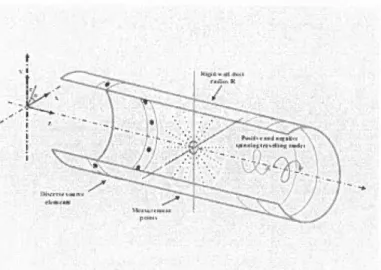
FREE-FIELD INLET / OUTLET NOISE

IDENTIFICATION ON AIRCRAFT ENGINES USING

MICROPHONES ARRA Y

By

1 man Khatami

Jury: Alain Berry (director) Noureddine Atalla

Patrice Masson Ninad Joshi

A Thesis Submitted for the Degree ofDoctor ofMechanical Engineering of

Université de Sherbrooke

UNIVERSITÉ DE SHERBROOKE

Faculté de génie

Département de génie Mécanique

IDENTIFICATION DU BRUIT D'ENTRÉE ET DE

SORTIE SUR DES MOTEURS D'AVION PAR

ANTENNES MICROPHONIQUES

Thèse de doctorat Spécialité : Génie Mécanique

Iman Khatami

Jury: Alain Berry (superviseur) Noureddine Atalla

Patrice Masson Ninad Joshi

Résumé

La présente thèse étudie la discrimination du bruit d'entrée/ de sortie des moteurs d'avion dans des tests statiques en champ libre en utilisant des antennes de microphones en champ lointain. Diverses techniques sont comparées pour ce problème, dont la fol1)1ation de voie classique (CB), la méthode inverse régularisée (régularisation de Tikhonov), la formation de voies généralisée inverse (L 1-GIB), Clean-PSF, Clean-SC et deux méthodes proposées qui s'appellent la méthode hybride et la méthode Clean-hybride. La méthode la formation de voie classique est désavantagée en raison de son besoin de nombreux microphones de mesure. De même, la

méthode inverse est désavantagée en raison du besoin d'information a priori sur les sources. La

régularisation Tikhonov classique fournit des améliorations dans. la stabilité de la solution; cependant elle reste désavantageuse en raison de son exigence d'imposer une pénalité plus fo1te pour des positions de source non détectées. Des sources cohérentes et incohérentes peuvent être résolues par la formation de voies généralisée inverse (Ll-GIB). Cet algorithme peut identifier les sources multi- polaires aussi bien que les sources monopolaires. Cependant, l'identification de source par la formation de voies généralisée inverse prend beaucoup de temps et exige un ordinateur avec une capacité de mémoire élevée. La méthode hybride est une nouvelle méthode

de régularisation qui implique l'utilisation d'untraitement par formation de voie a priori pour

définir une norme discrète et dépendante des données pour la régularisation du problème inverse. En comparaison avec la formation de voie classique et la méthode inverse, l'approche hybride (régularisation par formation de voie) fournit des cartographies améliorées d'amplitudes de sources sans aucune complexité supplémentaire substantielle. Bien que la méthode hybride lève les limitations des méthodes classiques, l'application de cette méthode pour l'identification de sources de faible puissance en présence de sources de forte puissance n'c:st pas satisfaisante.

On peut expliquer ceci par la plus grande pénalisation appliquée à la source plus faible dans la

méthode hybride, qui aboutit

à

la sous-estimation de l'amplitude de cette source. Pour surmonter

ce défaut, la méthode Clean-SC et la méthode Clean-hybrides proposée qui est une combinaison de la méthode hybride et de Clcan-SC sont appliquées. Ces méthodes éliminent l'effet des sources fortes dans les cartographies de puissance de sources pour identifier les sources plus faibles. Les méthodes proposées qui représentent la contribution principale de cette thèse

de toutes les approches est menée pour divers types de sources et de configurations microphoniques. Pour valider l'étude théorique, plusieurs expériences en laboratoire sont

réalisées à Université de Sherbrooke. Les méthodes proposées ont été appliquées aux données

de bruit mesurées d'une turbo-soufflante Pratt & Whitney Canada pour fournir une meilleure résolution spatiale des sources acoustique et une solution robuste avec un nombre limité des microphones de mesure comparé aux méthodes existantes.

Mots-clés : identification de source, bruit de moteur, inverse, hybride, Hybride-Clean, formation de voie.

Summary

This thesis considers the discrimination of inlet / exhaust noise of aero-engines in free-field static tests using far-field microphone arrays. Various techniques are compared for this problem, including classical beamforming (CB), regularized inverse method (Tikhonov regularization), LI- gencralized inverse beamforming (Ll-GIB), clean-PSF, clean-SC and two novel methods which are called hybrid method and clean-hybrid. The classical beamforming method is disadvantaged due to its need for a high number of measurement microphones in accordance with the requirements. Similarly, the inverse method is disadvantaged due to their need of ·

having a priori source information. The classical Tikhonov regularization provides

irnprovernents in solution stability, however continues to be disadvantaged due to its requirement of imposing a stronger penalty for undetected source positions. Coherent and

incoherent sources are resolved by L 1- generalized inverse bearnforrning (Ll-GIB). This

algorithm can distinguish the multipole sources as well as the monopoles sources. However,

source identification by L 1- generalized inverse beamforming takes much time and requires a

PC with high memory. The hybrid method is a new regularization method which involves the

use of an a priori beamforming measurement to define a data-dependent discrete smoothing

norm for the regularization of the inverse problem. Compared to the classical beamforming and the inverse modeling, the hybrid (beamforming regularization) approach provides improved source strength maps without substantial added complexity. Although the hybrid method rather solves the disadvantage of the former methods, the application ofthis method for identification of weaker sources in the prcsencc of the strong sources isn't satisfactory. This can be explained by the large penalization being applied to the weaker source in the hybrid method, which results in underestimation of source strength for this source. To overcome this defect, the clean-SC method and the proposed clean-hybrid method, which is a combination of the hybrid method and the clean-SC, are applied. These methods remove the effect of the strong sources in source power maps to identify the weaker sources. The proposed methods which represent the main contribution of this thesis show promising results and opens new research avenues. Theoretical

study of all approaches is performed for various sources and configurations of array. ln order

to validate the theoretical study, sever~\ laboratory experiments are conducted at Université de Sherbrooke. The proposed methods have further been applied to the measured noise data from

resolution and solution robustness with a limited number of measurement microphones compared to the existing methods.

Acknowledgment

lt is with immense appreciation that f acknowledge the support and help of my supervisor,

Professor Alain Berry, for his excellent guidance, caring, patience, and providing me with an excellent atmosphere for doing research. Without his guidance and persistent help this

dissertation would not have been possible. Also, f would like to thank NSERC, Research Chair,

P&WC for the financial support of this project. Last but not least, 1 would like to thank my lovely wifc, Maryam and my family for their wonderful support, guidance, and patience.

Table of Contents:

R,

_{esume ... 1}

.

Acknowtedgment ... V

CHAPTER t INTRODUCTION ... I

1.1

Context ... 1

t .2 Technological Problem

&

scientific problem ... 1

l .3 Objective ... 4

1 .3. l Task

(1):

Literature Review ... 4

l.3.2 Task (Il): Theoretical Study of Source Identification Algorithms ... 4

1.3.3 Task (t Il): Laboratory Test., ...

5

t .3.4 Task (IV): Application of Atgorithms to Real Engine Data ... 5

1. 4 Summary ...

5

2 CHAPTER 2 LITERA TURE REVIEW ... 7

2. 1 1 ntroduction ... 7

2.2 Literature Review of Noise Identification of Aircraft Engines ... 7

2.3 Applications of Sensor A rra y ... 13

2.4 Fundamental concepts of Array Processing ... 15

2.4. I Spatial Aliasing and Time Aliasing ... 16

2.4.2 Directivity ... 17

2.4.3 Near-Field and Far-Field ... 18

2.4 .4 Resol ut ion ... : 1 9

2.4.5 Mainlobe, Sidelobe and Gratelobe ... 19

2.4.6 Linear arrays ... 20

2.4.7 Circular Arrays ... 23

3 CHAPTER 3 SOURCE IDENTlFICATION METHODS

usrNG

MlCROPHONE

ARRA Y ... , .. ,., ... ~~ 27

3 .. 1 lntrod.uction ... 27

3.2 Source ldentification Methods Using Microphone Array ... 28

3.3 Beamforn1ing 1nethod ... 28

3.3.1 Classical Beamforming (CB) ... 28

3.3.2 Clean Be,amforming( Clean-PSF) ... 33

3.3.3 Clean Bcamforming (Clean-SC) ... 35

3.4 Inverse Problem ... 3 7 3.4.1 Classical Inverse method (Tikhonov) ... 3 7 3.4.2 Theory of L 1-generaliz.ed Inverse Beamfonnirng ... 42

3.5 The Hybrid Approach~ Beamforrning Regularization Matrix ..•.••••... .44

3.5. l Review of Hybrid Methods in Source ldentification ... 44

3.5 .. 2 Clean-Hybrid ... 4 7

3.6 Summary ... 48

4 CHAPTER 4 A lgorithm Development & Parametric Studies ... 50

4 .. 1 lntroduction ... ~~···5•••••••••••• 50 4.2 Theoretical conc~pts ...••••••••••••••••... 5 l 4.2.1 Sound field SjmuJation ... 51

4.2.2 M•crophone Array Cross Spectral Matrix ...

.5

l 4.2.3 Auto-Spectral Power of Sound Pressure ... 52

4.2.4 Directivity Simulation ... 53

4.3 Si1nuladon r-esults ... 53

4.3. I The Effect of Different Arroy Configurations on the Results ... 53

4.3.3 rdentification of Unequal Amplitude Sour-ces Using Diffcrcnt Algorithms ... 67

4.3.4 ldentmcation of Correlated

Sources.

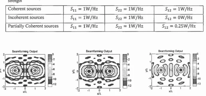
Uncorrelated Sources and Partially Correlated Source with Different Algorithms ... 70

4.3.5 ldentification of Monopole. Dipole and Quadrupole Sources with Different A lgor1thms ... : ···~ ... ~ ... ~ .... 74

4.3.6 Validation

of Source

Power Values with Theoretical

Method ...

74

4.3.7 Directivity ... 80

4.3.8 Comput:ational Cost of the Source Identification Methods ... 83

4.4 Summar}' ... 44· ···4· 4•··4••••444•~4 ·~~· ... ••••• ... 84

5 CHAPTER

5 VALJDATION THROUGH EXPERIMENTS

rN

CONTROLLED

CON Dl Tl 0 N S ...

4 4 4. 4 4 •• 4 . . . .. . .

85

5. 1 1 ntroduction ...•...••••• 85

5. 2 La boratory Tests ...•..•...•• 85

5.2.1

Description of the

Test

Set-up ... 85

Different Numbers I L<Xations of Loudspeakers ... 86

Various Sourc·e A mp 1 it:udes ... 1 •1 . . . ... ... .. 86

Correlated/U nco rre lated Sources ... 86

5

.3

Experiments with Loudspeakers ... 87

5.3.1 Validation of the Methods for Different Configuration of Microphones ... 88

5.3.2 Validation of the Methods with Different Numbers and

Locati.ons

of

Loudspeakers. ...

~

...

4 4 . . ... . . . 9 5 5.3.3 Validation of the Methods for Speakers i.vith Different Amplitudes ... 101

5.3.4 Validation of the Methods for Correlated and Uncorrelated Sources ... 104

5 .4 Ex per i ment wir h the W avegu ide System ... l 08 5.4.1 Va1idation of the Methods for DUTerent Configurations of Array ... 108 5.4.2

Validation

of the Methods for Different Frequencies ... 1 l.4

5.4.3 Reconstruction of the Directivity of Waveguide System ... 118

5.4.4 Sumrnary ... J 20 6 CHAPTER 6 APPLICATION TÇ) ENGINE DA TA ... 121

6.1 Real Engine Test ... 121

6.1. l Sound Measurement ... 121

6.1.2 Sound Identification of Inlet/Outlet Engine at Single Frequencies ... 123

6.1.3 Sound Identification of lnlet/Outlet Engine in 1 /3 Octave Frequency Bands ... 127

6.1.4 lnlet/ Aft Separation of Engine Noise ... 131

6.2 Summary ... 133

7 CHAPTER 7 CONCLUSION AND RECOMMENDATIONS .... : ... 134

7.1 Conclusions ... : ... 134

7 .2 Recommendations and Further Research ... 136

CONCLUSION EN FRANÇAIS ... 137

Recommandations et Perspectives ... 13 8 A. Simulation of the Actual Engine Test con figuration ... 139

8 Bibliography ... 143

Table of Figures:

Figure 1.1: Maximum noise of aero-engine parts (J ulliard, 2006) ... 3

Figure 1.2 : Directivity plot of a plane wave in 300 ... 3

Figure 2.1 : Drawing of fan rig; the mode detection array is located on the grey strip in the intake (fan and array diameter ±80 cm, array ±40 cm ahead of the fan) (Sijtsma, 2007) ... 8

Figure 2.2 : Schematic diagram of the set-up considered with the source and microphone positions into a hard-walled infinite duct (Bravo & Maury, 2007) ... 9

Figure 2.3 : Geometry for polar correlation applied to jet noise (Fisher, et al., 1977) ... 9

Figure 2.4: Positions of the line array of microphones and of the aeroengine. The line array is longer in the forward arc (x > 0) than in the rear arc. The jet is on the left side of the figure and extends substantially past the left end of the array (Michel, 2008) ... 10

Figure 2.5: Positions of the line array of microphones and of the aeroengine. The line array is longer in the forward arc (x > 0) than in the rear arc. The jet is on the left si de of the figure and extends substantially past the left end of the array (Siller, et al., 2008) ... \ l Figure 2.6: Test rig and microphone in facility in the NASA John H. Glenn Research Center

(Glenn & Bridges, 2004) ... 12

Figure 2.7: (a): Test setup, (b): 30 beamforming grid (Dougherty & Podboy, 2009) ... 12

· Figure 2.8 : Picture from the south of the YLA array, showing the Y configuration of the individual sensors. Image courtesy of National Radio Astronomy Obscrvatory / Associated Univcrsities, lnc. I National Science Foundation (Malphrus, 1996) ... 15

Figure 2.9 : Two different sinusoids that fit the same set of samples (black spots) (Ti me Aliasing) ... 16

Figure 2.10 : Signal time sampi ing representation. The continuous signal is represented in a green color whereas the discrete samples are in blue ... 17

Figure 2.11 : Effect of aliasing in spatial domain ... 17

Figure 2.12 : (left) Monopole, (Right) Dipole ... 18

Figure 2.13 : (left) Spherical wave (Right) Plane wave ... 19

Figure 2.14 : Mainlobe sidelobes and gratelobe ... 20

Figure 2.15 : spherical co-ordinate and direction of source ... 20

Figure 2.16 : Linear array, broad side (left) and endfire (right) ... 21

Figure 2.17 : Effect of inter- element spacing (grating lobe) for end tire linear array ... 22

Figure 2.18 : End fire (left) and Broad side (right) linear array fors

=

,1,.4 and for a six-microphone array ... 22

Figure 2.19 : Schematic of circular array ... 24

Figure 2.20 : Oth order ordinary Bessel fonction UO) in dB ... 25

Figure 2.21 : Effect of inter- element spacing (grating lobe) for a uniform circular array ... 25

Figure 2.22 : Beamforming shape variation for circular free-field a rra y ... 26

Figure 3.1.Acoustic sources inscribed in volume Ys are identified using a set of sound pressure measurement points. Any field point is described by

x.

A point which belongs to the source volume Ys is denoted

y.

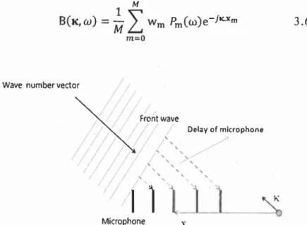
Microphone mis located in Xm ... 28

Figure 3.2. A microphone array, a far-field focus direction, and a plane wave incident from the focus direction ... 30

Figure 3.3. ln near-field focusing, spherical waves emitted by a monopole source at the focus point y are assumed. Signal delays are computed according to Equation 3.9 (Brüel&Kjrer, 2004) ... 3 l Figure 3.4: (a) Beamforming output for N=20, (b) Beamforming output for N=I OO ... 33

Figure 3.5: Camparison of beamforming and clean-PSF for sources that have a ... 35

Figure 3.6: Application of clean-SC for coherent sources (N=30,f= I 000Hz,R=5m) ... 37

Figure 3.7: Inverse method, (a) for SNR=IO and (b) SNR=l ... .40 Figure 3.8: Parametric representation of the residual norm vs. the regularized solution norm.42 Figure 4.1: Different configurations of array: (Left) Half-circular array, N

=

30, ( center) Fu

11-Figure 4.2: Conventional beamforming output for different configurations of array: (Left) Half-circular array, N

=

30, (center) Full-circular array, N

=

30, (Right) Full-circular

array, N

=

60 ... 55

Figure 4.3: Regularized inverse method output for different configurations of array: (Left) Half-circular array, N = 30, (center) Full-circular array, N = 30, (Right) Full-circular array, N

=

60 ... 55

Figure 4.4: Hybrid method output for different configurations of array: (Left) Half-circular array, N = 30, (center) Full-circular array, N

=

30, (Right) Full-circular array, N

=

60 ... 55

Figure 4.5: L 1-generalized inverse beamforming output for diffcrcnt configurations of array: (Left) Half-circular array, N

=

30, (center) Full-circular array, N = 30, (Right) Full-circular array, N = 60 ... 56

Figure 4.6: Clean-PSF output for different configurations of array: (Left) Half-circular array, N = 30, (center) Full-circular array, N = 30, (Right) Full-circular array, N = 60 ... 56

Figure 4.7: Clean-SC output for different configurations of array: (Left) Half-circular array, N

=

30, (center) Full-circular array, N = 30, (Right) Full-circular array, N

=

60 ... 56

Figure 4.8: Clean-hybrid output for different configurations of array: (Left) Half-circular array, N = 30, (center) Full-circular array, N = 30, (Right) Full-circular array, N = 60 ... 56

Figure 4.9: Schematic representation of the concept of API (Holmes, et al., 2005) ... 57

Figure 4.10: Conventional beamforming for 60 microphones and 800 microphones, for scan zone -20À

<

x

<

20,l, -20À.

<y<

ZOÀ. ... 59

Figure 4.11: Conventional beamforming for 60 microphones and 800 microphones, for scan zone -2À.

<

x

<

2À., -2À.

<y<

ZÀ. ... 59

Figure 4.12: Conventional beamforming output, (Left): Near-field configuration, (Right): Far-field configuration ... 60

Figure 4.13: Regularized inverse method output, (Left): Near-field configuration, (Right): Far-field configuration ... 60

Figure 4.1.4:Hybrid method output,(Left): Near-field configuration, (Right) : Far-field configuration ... 61

Figure 4.15: Ll-GIB, (Left): Near-field configuration, (Right) : Far-field configuration ... 61

Figure 4.16: Clean-PSF, (Left):Near-field configuration, (Right) : Far-field configuration ... 61

Figure 4.17: Clean-SC, (Left):Near-field configuration, (Right) : Far-field configuration ... 61

Figure 4.18 :Clean-hybrid: (Left):Near-field configuration, (Right) : Far-field ~on figuration .. 62

Figure 4.19: Configuration of array, N=60, R=132A, 2dA

=

28.6618 ... 62

Figure 4.20 : Conventional beamforming output of different number of sources, Left: One monopole source (source location is [0,0]), Center: Two monopoles sources with the same amplitude, Right: Three monopole sources with the same amplitudes ... 64

Figure 4.21: Regularized inverse method output of differcnt number of sources, Lcft: One monopole source, Center: Two monopoles sources with the same amplitude, Right: Three monopole sources with the same amplitudes ... : ... 64

Figure 4.22 : Hybrid output of different number of sources, Left: One monopole source, Center: Two monopoles sources with the same amplitude, Right: Three monopole sources with the same amplitudes ... 64 Figure 4.23 : L 1-general ized inverse beamforming output of different number of sources, Left: One monopole source, Center: Two monopoles sources with the same amplitude, Right: Three monopole sources with the same amplitudes ... 65 Figure 4.24:Clean-PSF output of different number of sources, Left: One monopole source, Center: Two monopoles sources with the same amplitude, Right: Three monopole sources with the same amplitudes ... 65 Figure 4.25 : Clean-SC output of different number of sources, Left: One monopole source, Center: Two monopoles sources with the same amplitude, Right: Three monopole sources with the same amplitudes ... 65 Figure 4.26: Clean-Hybrid output of different number of sources, Left: One monopole source, Center: Two monopoles sources with the same amplitude, Right: Three monopole sources with the same amplitudes ... 66

Figure 4.27:Three monopole sources with equal amplitudes at [ÀS O], [-ÀS O], [0,3,15], ... 67

Figure 4.28 : Conventional beamforming method in the case of two uncorrelated broadband inputs with a 6dB level difference ... 68 Figure 4.29: Regularized inverse method in the case of two uncorrelated broadband inputs with a 6dB level difference ... 68 Figure 4.30: Hybrid method in the case of two uncorrelated broadband inputs with a 6dB level difference ... 68 Figure 4.31 : L 1-generalized inverse beamforming method in the case of two uncorrelated broadband inputs with a 6dB level difference ... 69 Figure 4.32:Clean-PSF method in the case of two uncorrelated broadband inputs with a 6dB level difference ... 69 Figure 4.33 : Clean-SC method in the case of two uncorrelated broadband inputs with a 6dB Ievel difference ... 69 Figure 4.34: Clean-hybrid method in the case of two uncorrelated broadband inputs with a 6dB Ievel difference ... 70 Figure 4.35: Output of conventional beamforming for, Left: Two uncorrelatcd sources, Centcr: Two partial ly correlated sources, Right: Two full y correlated sources ... 71 Figure 4.36 : Regularized inverse output for two monopole sources, Left: Two uncorrelated sources, Center: Two partially correlated sources, Right: Two fu lly correlated sources ... 71 Figure 4.37: Hybrid method output for two monopole sources, Left: Two uncorrelated sources, Center: Two partial\ y correlated sources, Right: Two full y correlated sources ... 72 Figure 4.38: L 1-generalized inverse beamforming output for two monopole sources, Left: Two uncorrelated sources, Center: Two partially correlated sources, Right: Two fully correlated sources ... 72 Figure 4.39: Clean-PSF output for two monopole sources, Left: Two uncorrelated sources,

Figure 4.40: Clean-SC o_utput for two monopole sources, Left: Two uncorrelated sources, Center: Two partially correlated sources, Right: Two fully correlated sources ... 73 Figure 4.41: Clean-hybrid output for two monopole sources, Left: Two uncorrelated sources, Center: Two partially correlated sources, Right: Two full y correlated sources ... 73 Figure 4.42: (a): A dipole source at origin, (b): Two closely spaced monopoles of source strengths Ql and -Ql which perform as a di pole source ... 74

Figure 4.43: Geometry of a quadrupole source (Hansen, 2005) ... 76 Figure 4.44: Conventiona[ beamforming output:(left) one monopole(Sl 1 = 1) and one dipolc

source(S22 = 4), (Right) one quadrupole (Sl 1 = 1) and one dipole sources(S22 = 4) ·-··· 77

Figure 4.45 : Regularized inverse output:(left) one monopole and one dipole source, (Right) one quadrupole and one di pole source ... 77 Figure 4.46: Hybrid output:(left) one monopole and one dipole source, (Right) one quadrupole and one dipole source ... 78 Figure 4.47: Ll-generalized inverse beamforming output: (left) one monopole and one dipole

source, (Right) one quadrupole and one di pole source ···--78 Figure 4.48:Clean-PSF :(left) one monopole and one dipole source, (Right) one quadrupole

and one dipole source ... 78 Figure 4.49 : Clean-SC output:(left) one monopole and one dipole source, (Right) one

quadrupole and one di pole source ... 79 Figure 4.50: Clean-hybrid output:(left) one monopole and one dipole source, (Right) one quadrupole and one dipole source ... 79 Figure 4.51: grid point that covers two sources with different directivity ... 81 Figure 4.52:Source power map and directivity of two uncorrelated sources with same

amplitudes at f=l OOOHz, (a): Source power map of Beamforming, (b): Source power map of Clean-SC, (c): Directivity of sources by Beamforming, (d): Directivity of sources by Clcan-SC ... 82 Figure 4.53: Source power map and directivity of two uncorrelated sources with 6dB difforcnt amplitudes at f= lOOOHz, (a): Source power map of Beamforming, (b): Source power map of SC, (c): Directivity of sources by Beamforming, (d): Directivity of sources by Clean-SC ... 83 Figure 5.1: Schematic of test Laboratory test ... 86 Figure 5.2: Experimental set-up in the laboratory for loudspeakers without waveguides ... 88 Figure 5.3: four different configurations of array, (a): 188 microphone on full circular array where microphone distances are 6cm,(b): 94 microphones on semi-circular array, microphone distances are 6cm, (c): 94 microphones on full circular array, microphone distances are l 2cm, (d): 60 microphones on full circular array, microphone distances are l 8cm ... 89 Figure 5.4: Conventional beamforming output of the different configurations of array, (a): 188 microphone on full circular array (b): 94 microphones on semi-circular array, (c): 94

microphones on full circular array (d): 60 microphones on full circular array ... 90

Figure 5.5: Regularized inverse method output of the different configurations of array, (a): 188 microphone on full circular array (b): 94 microphones on semi-circular array, (c): 94

microphones on full circular array (d): 60 microphones on full circular array ... 90 Figure 5.6: Hybrid method output of the different configurations of array, (a): 188 microphone on full circular array (b): 94 microphones on semi-circular array, (c): 94 microphones on full circular array (d): 60 microphones on full circular array ... 91 Figure 5.7: Ll-GIB output of the different configurations of array, (a): 188 microphone on full circular array (b): 94 microphones on semi-circular array, (c): 94 microphones on full circular array ( d): 60 microphones on full circular array ... , ... 91 Figure 5.8: Clean-PSF output of the different configurations of array, (a): 188 microphone on full circutar array (b): 94 microphones on semi-circular array, (c): 94 microphones on full circular array (d): 60 microphones on full circular array ... 92 Figure 5.9: Clean-SC output of the different configurations of array, (a): 188 microphone on full circular array (b): 94 microphones on semi-circular array, (c): 94 microphones on full circular array (d): 60 microphones on full circular array ... 92 Figure 5.10: Clean hybrid output of the different configurations of array, (a): 188 microphone on full circular array (b): 94 microphones on semi-circular array, (c): 94 microphones on full circular array (d): 60 microphones on full circular array ... 93 Figure 5.11: loudspeaker orientations for: one speaker (left), two speakers (center) and two speakers (right) ... 95 Figure 5.12: Conventional beamforming output, (left): One source in the center ( center): Two source speakers by same amplitude at (75cm,O) and (-75cm, 0) , (right): Two source speakers by same amplitude at (30cm,O) and (-30cm, 0), F""' 1 kHz ... 96 Figure 5.13: Regularized inverse method output,(left): One source in the center (center): Two source speakers with equal amplitude at (75cm,O) and (-75cm, 0), (right): Two source

speakers with equa\ amplitude at (30cm,O) and (-30cm, 0), F=l kHz ... 96 Figure 5.14: Hybrid method output, (left): One source in the center (center): Two source speakers with equal amplitude (75cm,O) and (-75cm,O), (right): Two source speakers with equal amplitude at (30cm,O) and (-30cm,O), F= 1 kHz ... 96 Figure 5.15: Ll-generalized inverse beamforming output, (left): One source in the center (center): Two source speakers with equal amplitude at (75cm, 0) and (-75cm, 0), (right): Two source speakers with equal amplitude at (30cm,O) and (-30cm, 0), F= I kHz ... 97 Figure 5 .16: C\ean-PSF output , (left): One source in the center ( center): Two source speakers with equal amplitude (75cm, 0) and (-75cm, 0) , (right): Two source speakers with equal amplitude at (30cm,0) and (-30cm, 0), F=lkHz ... 97 Figure 5.17: Clean-SC output,(left): One source in the center (center): Two source speakers with equal amplitude (75cm, 0) and (-75cm, 0) , (right): Two source speakers with equal amplitude at (30cm,O) and (-30cm, 0), F=I kHz ... 97

Figure 5.18: Clean-hybrid output,(left): One source in the center (center): Two source speakers with equal amplitude (75cm, 0) and (-75cm, 0) , (right): Two source speakers with equal amplitude at (30cm,O) and (-30cm, 0), F=I kHz ... 98 Figure 5.19: Conventional beamforming for two speakers at f=200Hz, with equal amplitudes at (30cm, 0) and (-30cm, 0) ... 99 Figure 5.20: Regularized inverse method for two speakers at f=200Hz, with equal amplitudes at (30cm, 0) and (-30cm, 0) ... 99 Figure 5 .21 :Hybrid method for two speakers at f=2001-lz, with equal amplitudes at (3 Ocm, 0) and (-30cm, 0) ... 99

Figure 5.22: Clean-PSF for two speakers at f=200Hz, with equal amplitudes at (30cm, O) and

(-30cm, 0) ... 1 OO Figure 5.23: Clean-SC for two speakers at f=200Hz, with equal amplitudes at (30cm, 0) and (-30cm, 0) ... 1 OO Figure 5.24: Clean-hybrid for two speakers at f=200Hz, with equal amplitudes at (30cm, 0) and (-30cm,0) ... IOO Figure 5.25: Conventional beamforming output for two source speakers with 6d8 relative levels, F=lkHz ... 101 figure 5.26: Regularized inverse method output for two source speakers with 6d8 relative [evels, F= 1 kHz ... 101 Figure 5.27: Hybrid method output fortwo source speakers with 6d8 relative \evels, F=lkHz

... 102 Figure 5.28: Ll-generalized inverse method output for two source speakers with 6d8 relative levels, F= lkHz ... 102 Figure 5.29: Clean-PSF output for two source speakers with 6dB relative levcls, F= 1 kHz ... 102 Figure 5.30: Clean-SC output for two source speakers with 6d8 relative levels, F= 1kHz ... 103 Figure 5.31: Clean Hybrid output for two source speakers with 6dB relative levels, F= 1 kHz

... 103 Figure 5.32: Conventional beamforming output, (left): Two correlated sources (right): Two uncorrelated sources, F= 1 kHz ... 105 Figure 5.33: Regularized inverse output(left): Two correlated sources (right): Two

uncorrelated sources, F= 1 kHz ... 106 Figure 5.34: Hybrid method output, (left): Two correlated sources (right): Two uncorrelated sources, F= 1 kHz ... 106 Figure 5.35: L 1-generalized inverse beamforming output, (left): Two correlated sources (right): Two uncorrelated sources, F"': I kHz ... 106 Figure 5.36: C\ean-PSF output, (left): Two correlated sources (right): Two uncorrelated sources, F= l kHz ... 107 Figure 5.37: Clean-SC output(left): Two correlated sources (right): Two uncorrelated sources, F=lkHz ... I 07

Figure 5.38: Clean-hybrid output(left): Two correlated sources (right): Two uncorrelated sources, F= l kHz ... 107 Figure 5.39:Experimental set-up in the laboratory for Waveguide system ... l 08 Figure 5.40 : Conventional beamforming output of the different configurations of array at f=l OOOHz, (a): 188 microphone on full circular array (b): 94 microphones on semi-circular array, (c): 94 microphones on full circular array (d): 60 microphones on full circular array .109 Figure 5 .41 : Regularized inverse method output of the different configurations of array at f=l OOOHz, (a): 188 microphone on full circular array (b): 94 microphones on semi-circular array, (c): 94 microphones on full circular array (d): 60 microphones on full circular array .11 O Figure 5.42: Hybrid method output of the different configurations of array at f= I OOOHz, (a): 188 microphone on full circular array (b): 94 microphones on semi-circular array, (c): 94 microphones on full circular array ( d): 60 microphones on full circular array ... 1 10 Figure 5.43 : L 1-generalized inverse beamforming output of the different configurations of array at f=IOOOHz, (a): 188 microphone on full circulararray (b): 94 microphones on semi-circular array, (c): 94 microphones on full semi-circular array (d): 60 microphones on full semi-circular array ... : ... 111 Figure 5.44: Clean-PSF output of the different configurations of array at f=I 000!-lz, (a): 188 microphone on full circular array (b): 94 microphones on semi-circular array, (c): 94

microphones on full circular array (d): 60 microphones on full circular array ... 111 Figure 5.45: Clean-SC output of the different configurations of array at f=l OOOHz, (a): 188 microphone on full circular array (b): 94 microphones on semi-circular array, (c): 94

microphones on full circular array (d): 60 microphones on full circular array ... 112 Figure 5.46: Clean-Hybrid output of the different configurations of array at f=I OOOHz, (a):

188 microphone on full circular array (b): 94 microphones on semi-circular array, (c): 94 microphones on full circular array (d): 60 microphones on full circular array ... 112 Figure 5.47: Conventional beamforming output for different frequencies, (a):200Hz,(b): 800Hz,( c ): 1 OOOHz, ( d):2000Hz ... 1 15 Figure 5.48: Regularized inverse method output for different frequencies, (a):200Hz,(b): 800Hz,(c): 1 OOOHz, (d):2000Hz ... : ... J l 5 Figure 5.49: Hybrid method output for different frequencies, (a):200Hz,(b): 800Hz,(c):

1 OOOHz, (d):2000Hz ... 116 Figure 5.50: Ll-GIB output for different frequencies, (a):200Hz,(b): 800Hz,(c): 1 OOOHz, (d):2000Hz ... , .... 116 Figure 5.51: Clean-PSF output for different frequencies, (a):200Hz,(b): 8001-lz,(c): 1 OOOHz, (d):2000Hz ... l l 7 Figure 5.52: clean-SC output for different frequencies, (a):200Hz,(b): 800Hz,(c): 1 OOOHz, (d):2000Hz ... l l 7 Figure 5.53:Clean-hybrid output for different frequencies, (a):200Hz,(b): 800Hz,(c): 1 OOOHz, (d):2000Hz ... , ... l J 8

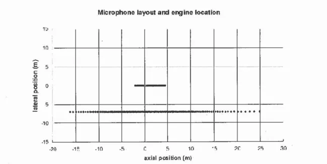
Figure 6.1: Free-field sound pressure measurements of a P&WC engine with 17 microphones

located at 45 m from the engine over a circular arc ... 122

Figure 6.2: Normalized Power spectral density of microphone at 20 O ... 123

Figure 6.3: : Normalized Power spectral density of microphone at 100 O ... 124

Figure 6.4: Conventional beamforming output for, Left: f=4 74Hz,Center:950Hz, Right: l 266Hz ... 124

Figure 6.5: Regularized inverse method output for, Left: f=474Hz,Center:950H~, Right: 1266Hz ... 124

Figure 6.6:Hybrid method output for, Left: f=4 74Hz,Center:950Hz, Right: l 266Hz ... 125

Figure 6.7: Ll-GIB output for, Left: f=474Hz,Center:950Hz, Right: 1266Hz ... l 25 Figure 6.8:Clean-PSF output for, Left: f=4 74Hz,Center:950Hz, Right: l 266Hz ... 125

Figure 6.9: Clean-SC output for, Left: f=4 74Hz,Center: 950Hz, Right: 1266Hz ... 125

Figure 6.10: Clean-hybrid output for, Left: f=474Hz,Center:950Hz, Right:l266Hz ... 126

Figure 6.11 :Directivity of source from microphone pressure for tonal frequencies ... 127

Figure 6.12: Conventional beamforming map for third octave band frequency ... 128

Figure 6.13: Regularized inverse method map for third octave band frequency ... 128

Figure 6.14: Hybrid method map for third octave band frequency . .' ... 129

Figure 6.15: Ll-GIB map for third octave band frequency ... 129

f-'igure 6.16: Clean-PSF map for third octave band frequency ... 130

Figure 6.17: Clean-SC map for third octave band frequency ... 130

Figure 6.18: Clean-hybrid map for third octave band frequency ... 131

Figure 6.19: Schematic of grid point area for the engine test (the directivity of in let source is obtained by the point sources in the red right rectangular and the directivity of aft source is obtained by the point sources in the red left rectangular) ... 132

Figure 6.20: Directivity of in let and outlet engine ... 133

Tables

Table 2.1: Various Fields of Application for Array Processing (Allred, 2006) ... 13

Table 4.1: Source power Value for three different configurations of arrays ... 57

Table 4.2: Modelled API for images with point source at (0, -Â.) ... 58

Table 4.3: Microphones distance and for each configuration ... 59

Table 4.4: Source power for different number of sources ... 66

Table 4.5: Relative Source power for two uncorrelated source with 6dB difference amplitude ... 70

Table 4.6: The value of auto spectral density of source strength and the Cross spectral density of source strength ... 71

'l'able 4. 7: Source power value ... 73

Table 4.8: Relation between SQQ with Sd and Sqfor different values of Dipole and Quadrupole ... 77

Table 4.9: Source power for multipole sources ... 79

Table 4.1 O.Computational cost of the Source identification methods ... 84

Table 5.1: Various Test validations in The Laboratory ... 86

Table5.2: Microphone distance ofvarious configurations (À2

=

0.175m,f

=

1000Hz) ... 94

Table 5.3: Source quantification for the different methods ... 94

Table5.4: Relative source power for two uncorrelated source with 6d8 difference in amplitude ... 104

Table 5.5 :Source quantification for correlated and uncorrelated sources ... 108

Table 5.6: Source quantification for the different methods at f=I OOOHz ... 113

Table 5.7:Wavelength ofdifferent frequencies ... 114

Table 5.8: Normalized source power of method for different frequencies ... 118

CHAPTER 1 INTRODUCTION

1.1 Context

This research is completed under the supervision of Professor A.Berry at Group d' Acoustique

de l'Universite de Sherbrooke. This research has been financially supported by Pratt & Whitney

Canada Corporation to discriminate inlet/outlet noises on aircraft engines using phase array methods in farfield condition. Base on the results, it will be possible to detect these noises by using the novel approaches with more resolution than the classical methods.

1.2 Technological Problem

&

scientific problem

The most evident environmental impact of airplanes is noise. The effects of noise on people motivate researchers to reduce aircraft noise. Aircraft noise is different at various flight conditions. The chief sources of aircraft noise occur in landing and taking off conditions. Although individual aircraft has become quieter in the recent past, tlight frequencies have increased. As a consequence, aircraft noise is giving rise to people's concern. Airplane noise leads to passengers or even airplane staff feeling stressed and irritated. Since this noise occurs continuously, it can be annoying despite its low amplitude. Airplane noise also incrcascs concern about air crashes for some passengers who are sensitive to aircraft noise. lnterference with sleep patterns is another problem which is frequently reported by people living near airports. A recent study of residents who are living close to airports, mentioned that between 1 in 5 and 1 in 10 people often report difficulty going to sleep or being woken early (Parliamentary Office of Science and Technology, 2003). In addition, certain evidence has been reported of mental illness occurring becau.se of noise. The question is how this noise is created. Compression and rarefaction of the air happens due to the moving aircraft which causes motion of air molecules. This movement of air molecules propagates pressure waves in the air and the pressure waves produce an unpleasant hearing for human. The airflow around the fuselage and control surfaces of the aircraft produce aerodynamic noise, and aircraft speed increases this type of noise. The main part of aircraft noise is occurred through engine especially during takeoff and climb when the speed of the tips of the fan blades is supersonic. The majority of engine noise is due to jet noise and turbofans. The moving parts of the engine are the main

reason behind the creation noise. The contact between flows with the moving parts produces unpleasant sound. To solve these problems, many studies have been carried to reduce aircraft noise. To reduce aircraft noise two main tasks must be performed:

1. Localization of sound sources

li. Finding a method in order to eliminate or at least reduce the noise

This study focuses on the first step of this goal, which will be explained in the next chapters. As mentioned, engine is the main part of airplane noise for which researchers have a special attention. Extensive work has been performed to deve\op the source identification methods in order to identify the various . noise sources of aero-engines (fan, compressor, turbine, combustion, jet exhaust). The relative significance of various noise of engine is shown in the Figure l. l (Jul\iard, 2006). This means the amplitudes of noise in different parts of engine are relatively different. This study attempts to estimate locations and amplitudes of'engine sources. The source identification methods are usually based on the phased array beamforming (Sijtsma, 2007), (Bravo & Maury.C., 2007) and (Michel, et al., 2006) or the inverse methods (Bravo &

Maury.C., 2007), (Michel, et al., 2006) and (Yoon & Nelson, 2000) have been implemented

using microphone arrays relatively close to the engine. The classical beamforming method is disadvantaged due to its need for a high number of measurement microphones in accordance to the requirements. Similarly, the inverse methods are disadvantaged due to their need of having an a priori source information. Researchers have applied a variety of algorithms to detect noise

sources and attempt to increase resolution and accuracy of source strength map by removing or filtcring side lobes (unreal sources) from this map. The sidelobes are unreal sources that cannot be distinguished from the mainlobe (real source) in the source power map. This effect is shown in Figure 1.2. A plane wave emerge from 30° which is shown by the mainlobe in directivity plot. However, several sidelobes are placed close to the mainlobe that cannot be distinguished from the main lobe. Consequently, researchers have attempted to find approaches that remove the sidelobes. Configuration of array is an important parameter which strongly affects source identification. There are several possibilities for array structure including linear array, grid array, circular array, etc. For. optimal performance, an attempt will be made in this study to find the best array configuration for this special case.

us

~

105 ;; > .:: •fan lnlet .È !ane•haust ! 95 _{Compr~sor core} :;

..

• Turbin~ "t: ... ~ 85 • J~I exhau>t

.~

~ 75 65 Aero-engine noise

Figure 1.1: Maximum noise of aero-engine parts (Julliard, 2006)

0 -10 -20 :ë"' ~ -30 - ~ ~ -40 0 -50 -60 .70.__~~~~~_._~..__._~_.___,'---_.__~_..___.._~~ 0 15 30 45 60 75 90 105 120 135 150 165 180 angle(degree)

Figure 1.2 : Directivity plot of a plane wave in 30°

ln this research, the aim is to discriminate noise in the in let and exhaust let of the aircraft enginc. ln the recent past, several studies have been implemented on noise identification in a!rcraft engine. However, in this project, we attempt to install a far field array configuration around the aircraft engine (approximately 45m) to detect the sources (location and amplitude) on aircraft. As earlier mentioned, classical methods (the conventional beamforming and the inverse method) have the drawbacks such as big sidelobes which cause incorrect identification of the sources. Therefore, this study attempts to apply an improved source identification method with higher resolution map that is suitable for far field array configuration. From the given discussion an

important question which has not been adequately answered previously is identified. This question is stated as follows:

What are the most accurate melhod and besJ configuration of array to identify in/et/out/et aero-engine noise in far:field condilion?

1.3 Objective

-This study specifically addresses the requirement for separation of noise sources emanating from the inlet and exhaust ducts of aircraft engines using far field microphone arrays. ln the problem under study, the acoustic data are provided by microphones distributed over a semi-circular arc at approximately 45m from a static engine stand. In this study, different algorithms are evaluated for source identification. A nove! hybrid method (Gauthier, et al., 2011), which is a combination of inverse modeling and conventional beamforming, is applied. Compared to conventional beamforming and inverse modeling, this approach provides improved source strength maps. However, this method doesn't always lead to reasonable results. For the hybrid method, identification of sources with low amplitude in presence of the strong sources is particularly difficult. Hence, to solve this imperfection, this navet method is combined with Clean-SC method. This method was initially investigated at Université de Sherbrooke for sound field extrapolation in small, closed environments based on sound field measurement with a microphone array. The method has proven to provide source localization in free-field, diffuse field and modal situations with better spatial resolution than conventional beamforming and inverse methods. To this end, the following tasks are designed.

1.3.1

Task (1): Literature Review

Conduct a literature review on previous studies which are related to the topic of this research

1.3.2

Task (Il): Theoretical Study of Source Iden.tification Algorithms

Review of classical source identification methods as well as the novel algorithms for simulation data. The hybrid method that builds upon the beneficial attributes of both the beam-forming and inverse methods is introduced. ln order to improve the resolution maps, the hybrid method combines with the clean-SC method. In other to achieve the best sound identification method and the best array configuration for the far-field condition, the simulation of various sources and configurations are evaluated.

1.3.3 Task (III): Laboratory Test

Validation of the methods with laboratory experiments on a test set-up that involves sound radiation from two co-axial waveguides and a circular array of microphones in a hemi-anechoic room. ln these experiments, the frequency content and magnitude of the sources were varicd as well as microphone array configurations in order to test the source identification algorithms and determine the promising array configurations for this prob\em.

1.3.4 Task (IV): Application of Algorithms to Real Engine Data

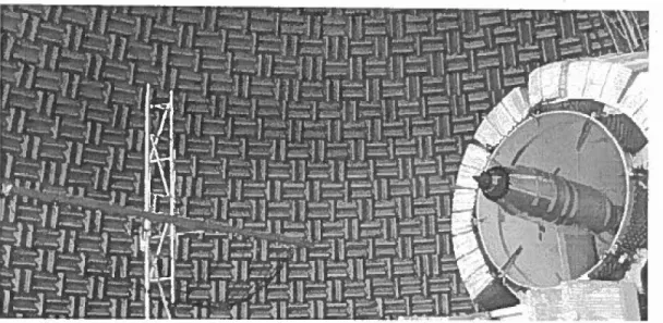
ln order to measure inlet/outlet noise in aircraft engine, Pratt & Whitney Canada Corporation

according to the simulation and the laboratory results, installed an array of microphones around the turbofan engine in far-field condition. Far-field engine noise testing is a standard procedure in the development cycle of any turbo-fan engine. The testing is done using a sem i-circular array of microphone installed a fixed distance from the engine. Separating the noise recordcd at the ground microphone location and accounting the contribution from the inlet and exhaust noise source is often required to have a more refined estima te of the aircraft noise and to create noise reduction strategies.

The best source identification methods validated in sections Il and III were tested and validated using the measured static noise data for a medium-bypass ratio turbo-fan engine, provided by Pratt and Whitney Canada Corporation.

1.4 Summary

ln this chapter the importance of source identification of aero-engine was presented. ln addition, the main tasks of this study were explained. Chapter 2 provides a literature review of array

methods. lt also reviews previous source identification methods which have been applied to

detect aircraft engine noises. Moreover, the concept of array (important paramcters) is explained in the rest of the chapter. Chapter 3 introduces theories of array techniques which are applied in this study. Chapter 4 deals with simulation results that demonstrate performance of various algorithms. ln this chapter, we simulate various types of sources including monopole, di pole, quadrupole, coherent and incoherent sources. The goal of these simulations is to examine the effectiveness of the source identification methods for the detection of the known simulated sources. ln Chapter 5 the source identification methods and the best array configuration are validated using laboratory experiments on a test set-up that involves sound radiation from two

co-axial waveguides and a serni-circular array of microphones in a hemi-anechoic room. This helps us in finding the satisfactory algorithms for our research. Chapter 6 discusses application of the algorithms to real engine tests. The engine tests data are applied to the best algorithm in order to detect sources in inlet/exhaust air craft engine. Finally, Chapter 7 summarizes the contributions and future directions.

CHAPTER 2 LITERA TURE REVIEW

2.1 Introduction

This chapter provides a briefbackground of sensor arrays and their application before reviewing previous studies on noise identification in aircraft engine using phased-array methods. Finally, some essential concepts of array will be explained.

2.2 Literature Review of Noise Identification of Aircraft Engines

Sijtsma has studied the feasibility of noise source location by phased array beamforming in engine ducts (Sijtsma, 2007). By advanced array techniques, broadband and tonal noise sources were identified. He applied the beamforming algorithm for fan rig measurements with a microphone array upstream of the fan (see Figure 2.1 ). The main goal of this study was to process tonal noise and broad band noise separately and also to apply the beamforming on stationary source and rotating sources. The circular array was applied to azimutal mode detection. Since the beamforming for this circular array doesn 't give any information about the axial position of the sound sources, a number of parallel microphone rings in the intake were

used. This new configuration partially salves this disadvantage and it can be partly rcmoved,

cspecia\ly at the higher frequencies. To examine the effects of an intake liner, a simulation study was implemented. Using a Green' s function in a lined tlow duct, synthesized microphone data is obtained. This liner is extremely essential for acquiring satisfactory the beamforming results. However, the liner properties are not critical for this. The simulations also demonstratedthat the inlet mode detection doesn't have axial resolution.

I \ 1 . 1 • . microphone 1 ' array \.,

..

/ ~' i I

Figure 2.1 : Drawing of fan rig; the mode detection array is located on the grey strip in the intake (fan and array diameter ±80 cm, array ±40 cm ahead of the fan)

(Sijtsma, 2007)

T.Bravo et.al tested the beamforming and the inverse methods for the localization of in-duct

sources (Bravo & Maury, 2007). A circular array of microphones was modeled in a cross section

of the circular duct and source elements were also assumed on the duct walls (Figure 2.2). They compared both methods according to two parameters: the axial distance between the array and the sources, and the frequency range. The performances of different beamforming techniques and regularized inverse method for identification of coherent and incoherent sources have been tested. The results show that when the sources are highly correlated or when the frequency is low, beamforming behaves poorly. The inverse method is less sensitive to the degree of coherence between the sources and has the advantage of providing correct source strength amplitude.

Figure 2.2 : Schematic diagram of the set-up considered with the source and microphone positions into a hard-walled infinite duct (Bravo & Maury, 2007). M.J.Fisher and co-workers have applied the polar correlation method for the localization of sources in aero-engine jet (Fisher, et al., 1977). They set up an array of far field microphones on a polar arc surrounding the jet (See Figure 2.3). This technique can be used to derive the complex source strengths of a continuous distribution of uncorrelated sources representing jet noise in the frequency domain, from the complex sound pressures readings over a circular arc and their cross-spectral power density.

jet

Mietcphone s~p.ir~tion angle

...-'7'0 Po la ra rc radius ---y µ "'.---=--..:~ Ml ... . ... ~··

..

-"'" /Ml ...•..•. / _,,., .. "" .... ·'

Figure 2.3 : Geometry for polar correlation applied to jet noise (Fisher, et al., 1977)

Michel (Michel & Funke, 2008) compared inverse methods with conventional beamforming for the source distribution a long the axis of a high bypass ratio aeroengine. They used a linear array of 128 microphones parallcl to the engine axis in an open air test. Figure 2.4 shows the microphone positions in relation to the location of the engine. For estimation of unknown source strengths, the matrix of the cross-spectra of the microphones with a set of assumed monopole point sources along the engine axis was used. They demonstrated that for a high bypass ratio aeroengine, both the source strengths and the directivities of all sound sources can be obtained.

The measurement was made in an open air test bed with a line array o( microphones which are

parallel to the engine axis in the geometric near field of the engine. Results show that inverse method has a far superior source resolution capability than the beamforming map in low frequency.

Microphone layout and engine location

1:.i 10

...

.5. 5 c: 0 :i:> ·~ 0 o. ~ .!!! 5 "' • • ···-~-. . . . -~~-. . . - . . . --~··· • • • • 1 ·10 .15 -?1) .10 10 .10 axial position (m)

Figure 2.4 : Positions of the li ne array of microphones and of the aeroenginc. The line array is longer in the forward arc (x > 0) than in the rear arc. The jet is

on the left side of the figure and extends substantially past the left end of the array (Michel, 2008).

Si lier et.al discussed the application of microphone antennas for acoustic indoor tests of aircraft engines (Si lier, et al., 2008). Such tests are conducted in the development phase of engines in order to identify and solve specific noise problems. A linear microphone array was installed on

special arrangement, the effect of sound waves retlected by the chamber walls has been minimized. The test was carried out at the indoor engine test facility of Lufthansa Technik in Hamburg. The microphone cross-spectral matrices are the input of the beamforming algorithm in the frequency domain. On the engine inlet region, a sub-array of microphones was focused. This sub-array was movable and by moving the sub-array along the linear array (advancing by one microphone at each step), they obtained the directivity of the cngine in let.

Figure 2.5 : Positions of the line array of microphones and of the aeroengine .

The line array is longer in the forward arc (x > 0) than in the rear arc. The jet is

on the left side of the figure and extends substantially past the le ft end of the array (Siller, et al., 2008)

Glenn et.al investigated jet noise source localization using a linear phased array (Glenn & Bridges, 2004). The main purpose of this research was to localize aero acoustics sources in aircraft exhaust jet. Two model engine nozzles were tested for various power cycles. 16 B&K 4135 microphones array was installed para\lel to the jet axis. Figure 2.6 shows the schematic of this test. Both conventional and minimum variance (for highest spatial resolution) beamforming are applied for this experiment. The beamforming approach evaluates the noise source distributions along the jet at different frequencies. The effect of free jet flow on jet noise distribution and also the effect of phased array distance from the jet on the resolution were investigated. The results show that by increasing the distance of array from the source, the spatial resolution is decreased.

Figure 2.6: Test rig and microphone in facility in the NASA John H. Glenn Research Center (Glenn & Bridges, 2004)

Recently deconvolution methods and matrix analysis approaches have been applied to improve source identification. Two fondamental advantages of deconvolution methods are improved spatial resolution and decreased sidelobes in low frequency. Matrix analysis methods are able to statistically separate independent sources. R.P.Dougherty set up a cylindrical cage array surrounding the jet to detect noise sources in the jet structure (Dougherty, 2010). Yarious beamforming algorithms were implemented to the cage array in this study: Classical Beamforming, 30 Clean-SC (Sijtsma, 2007), DAMAS (Brooks & Humphreys, 2006), TrDY (Dougherty & Podboy, 2009). The cage array configuration is shown in Figure 2. 7a). 16 transverse planes forming a 30 beamforming grid was assumed to reconstruct the noise sources (Figure 2.7b). n) b) 3 2 Ill .... .! ₀

Ë

;.; _·1 ·2 .3 .3 ·2 . \ •

. . .. .. . .. . .. .

..

.

..

.

..

. .

0 2 3 4 5 z, meters

The results clearly showed improvement of resolution in low frequency as compared to conventional beamforming. Source strength maps showed that for Clean-SC noise is located on the axis while for DAMAS, this noise is placed on a ring near the outer nozzle lip line. TIDY method results showed that locations of the noise are on both the axis and the shear Jayers.

2.3 Applications of Sensor Array

ln this section, a review of the history of sensor arrays in different fields is provided. ln Table 2.1, some fields of array applications are listed. Sorne of these applications are briefly dcscribed below. Although all of the listed applications employ arrays of sensors, they al! do in different manners (Allred, 2006). This means that they apply their own type of propagating energy using specific types of transducers or sensors which are sui table for the medium where energy propagates. Accordingly, the improvement ofthese array processing applications is donc separately and distinctly for each field.

Table 2.1: Various Fields of Application for Array Processing (Allred, 2006).

Application Field Description

Radar (Brookner, 1985) , (Haykin, Phased array radar, air traffic control, 1985) and (Munson, et al., 1983) and synthetic aperture radar

Sonar (Knight, et al., 1981) and Source localization and classification (Haykin, 1985)

Communications (Mayhan, 1976) and Directional transmission and reception (Compton, 1978)

Geophysical exploration (Justice & Earth crust mapping and oil exploration Havkin, 1985)

lmaging (Macovski, 1983), (Pratt, 1978) Ultrasonic and homographie and (Kak & Haykin., 1985)

Astronomy (Readhead, 1982) and (Yen, High resolution imaging of the uni verse 1985)

Biomedicine (Widrow, 1975) Fetal 1 _{heart monitoring and hearing aids}

Damage detection (NOT and SHM) Extraction of damage-sensitive features frorn a rra y (Stepinski & Uhl, 2013) measurements

Using antenna to improve high frequency transmission and reception in radars is common (Yan.Trees, 2002). Radar systems were popular among the military during World War Il and

were used as a defense against airborne attacks. However, non-military uses were expanded as well as military uses. Primai radar systems contain a directional antenna (parabolic dish) and steering was done mechanically for these radars to illuminate space and detect objects within range. ln other words, radars rotate with possible variations in elevation to detect the objects.

One way to coll~ct and retlect more radiation from abjects was using large antennas. Howcver

these larger arrays were more ponderous. As a consequence, using them in mobile platforms (ships, planes) was restricted. To overcome this limitation, phased-array antennas (multiple antennas) are placed together and for each antenna a phase shift is applied. Then the shifted signais are added together. The advantage of the multiple antennas is that by control\ing the phase shifts of the individual antennas, the direction of the array could be changed without physical\y varying the orientation of the antenna itself. The application of delay-and-sum beamforming method is similar to these array antennas. ln the past, phased-array antennas mechanical ly adjusted phase to steer its beam (Knittel & Oliner, 1972). However, electronical !y steered phased arrays were gradually replaced by mechanically steered phased arrays (Van.Trees, 2002). Sonar (Sound Navigation and Ranging) was another product which was used in the war as well as radar. The application of arrays in sonar is similar to that in radar. The main difference of sonar and radar is that acoustic energy is measured and sonar is applied in water, not air. Both active sonar and radar transmit energy and look at retlections that are receivcd. The energy transmitted can be phase aligned towards a particular direction by the array of sensors. The received signais can also be aligned to listen in that same direction (Cox, 1974). An array of sensors is required for passive sonar to listen to the environment to identify objectives. The advantages of passive sonar are that the ships which used passive sonar techniques can remain undetected, whereas active sonar gives the location of the ship going active away. For example, a submarine transmitting active sonar can easily be located by a ship which uses passive sonar. Another application of array is wireless communications (Feldman & Friis, 1937). Today, arrays are commonly used in many communications systems such as satellites, cellµlar telephone systems, and interplanetary communications. The advantagc of these phased-array antennas is the decreasing efficiency of multi-path propagation, interference from other sources, and receiver noise. Recently, these array systems have been applied for smaller and also simpler system to be useful for communication systems (Godara, 1997). The application of array in mobile devices is to track and direct the energy transmitted and received.

This can be possible with smart array (L.G.Godara, 2004). The goal of using sensor array in the field of astronomy is to analyze radio radiation from the universe. In radio astronomy, the

wavelengths are extremely longer than optical wavelengths (Graham-Smith & Burke, 1997). As

a consequence the size of the radio telescopes (the sensor apertures) must be larger by the same factor. The sensors are chosen larger in order to improve angular resolution. Since there are limits in building large telescopes, or sensors, multiple sensors spread over a larger area is advised. Radio interferometry was the tirst application of multiple sensors which was carried out Martin Ryle of Cavendish Laboratory of Cambridge University during World War Il. Aperture synthesis is another technique which uses multiple sensors. This technique makes use of the earth's rotation. The Very Large Array (VLA) which is shown in Figure 2.8, is a multiple array (the radio telescope array) that makes use of this technique.

Figure 2.8 : Picture from the south of the VLA array, showing the Y configuration of the individual sensors. Image courtesy of National Radio Astronomy

Observatory / Associated Universities, Inc. I National Science Foundation

(Malphrus, 1996).

2.4 Fondamental concepts of Array Processing

In this section some of the fondamental concepts of antenna theory are mentioned. Sorne basic detinitions for directional antennas are provided along with a discussion of the application of

linear array and circular array. Finally, Fourier Transform rnethod which is used for changing tirne domain to frequency domain is discussed.

2.4.1 Spatial Aliasing and Time Aliasing

Aliasing is a parameter which has significant effect on the results of the source identification

methods. In order to distinguish the different signais or a/iases of one another during the

sampling, it is necessary to pay attention to the aliasing pararneter. Aliasing also causes distortion or artifact results when a reconstructed signal from samples is not identical with the original continuous signal (see Figure 2.9). Figure 2.10 shows a time domain signal which is sampled with a constant rate

fs

=

1/T5 • To unambiguously reconstruct signais, the highest

frequency must be fN

=

fs/2

=

l/2T₅ (or the corresponding angular frequency, UJN

=

2rrfN

=

n/T₅ with a period of TN

=

2T_{5 )} which is called Nyquist frequency (Manolakis & Proakis, 1996). If we spatially sample a signal using microphone array with a sampling interval equal to

d, the spatial Nyquist angular frequency will be KN = rr/d with a period length equal to 2d.

Figure 2.1 1 demonstrates the effects of aliasing in the spatial domain. The figure i llustrates that if sampling is below the Nyquist rate, reconstruction won't be perfect; part of the signal overlaps with the next periodic signal. As a result, in the overlap places the values of the frequency add together and the shape of the signais will be quite different frorn the original signal.

:n,'~!f'\'

f

\K,r\~._:i\

ff7\-1

rrr\1

,. ,

1 1 ! 1

i \ \ . \ I

1 !

i

1 1

' /

i 11

i

"'·1 1 _{\ : ' 1 \ ·, \ \ /,}

.,ï \

1 \

f \

f \

j

i

/1\\

1

1 ; 1 \ ./ \

-O•·

1 '

1 \

1

-~J

\/

1

Vi (

1

·.:Lv -, v __

\~_J_~JJ_ V~-

\

1

;vv _

_\

Figure 2.9 : Two different sinusoids that fit the same set of samples (black spots) (Time Aliasing)

Figure 2.10 : Signal time sampling representation. The continuous signal is represented in a green color whereas the discrete samples are in blue

I , ~\ - \ . -411 -3rr -2rr -rr d d d d Aliasing

\

-

\., -4rr -3rr -211 -rr d d d d n -d

s

-

i Il d 211 d 211 d 311 d 3 d

Figure 2.11 Effect of aliasing in spatial domain

2.4.2 Directivity

4rr

d

Directivity is a fondamental parameter for array si,gnal processing. Directivity measures and iilustrates the radiation pattern of sound sources. For example a monopole source equally radiates sound in ail directions white for a dipole source, sound radiation is not identical in ail directions (see Figure 2.12). For a di pole source, sound radiation in two regions is strong while for two other reg ions they are cancel led.

Oipole

270

Figure 2.12 : (left) Monopole, (Right) Dipole

The radiation intensity of these so~rces F(8,</>) is defined is given as a function in spherical

coordinates (see Figure 2.15). The average radiation Fave for ail directions is given by:

1

r2Tr

LTr

Fave = _4n:

Jo

0 IF(8,

</>)1

2 _{sin 8d8d</>} 2.1

Mathematically, the formula for directivity (D) is written as:

D _ F(8,<J;) _

F(8,</J)

-

Fave -

4

~f

0

2

n:J

0

rclF(8,</J)l2sin8d8d<J;

2.2

The numerator of Equation 2.2 is the maximum value of F, and the denominator presents the "average power radiated over ail directions". This equation calculates the directivity of the source by measuring the peak value of radiated power divided by the average.

2.4.3 Near-Field and Far-Field

If the point of observation is far from a sound source, the assumption that the amplitude of the wave everywhere on the plane perpendicular toits direction oftravel (in the near vicinity of the observer) is the same would be reasonable. This type of wave is called a plane wave and formulas of far-field phase array methods are derived from plane wave assumption. ln othcr words, when wave front curvature is negligible, plane wave cou Id be used instead of spherical wave. A plane wave is an idealization that allows us to assume that the entire wave is traveling in a single direction, instead of spreading out in ail directions. On the contrary, if the point of