HAL Id: hal-01091283
https://hal.inria.fr/hal-01091283
Submitted on 5 Dec 2014
HAL is a multi-disciplinary open access
archive for the deposit and dissemination of
sci-entific research documents, whether they are
pub-lished or not. The documents may come from
teaching and research institutions in France or
L’archive ouverte pluridisciplinaire HAL, est
destinée au dépôt et à la diffusion de documents
scientifiques de niveau recherche, publiés ou non,
émanant des établissements d’enseignement et de
recherche français ou étrangers, des laboratoires
Verifying Modal Workflow Specifications Using
Constraint Solving
Hadrien Bride, Olga Kouchnarenko, Fabien Peureux
To cite this version:
Hadrien Bride, Olga Kouchnarenko, Fabien Peureux. Verifying Modal Workflow Specifications Using
Constraint Solving. The 11th International Conference on Integrated Formal Methods, IFM’2014, Sep
2014, Bertinoro, Italy. pp.171 - 186, �10.1007/978-3-319-10181-1_11�. �hal-01091283�
Verifying Modal Workflow Specifications
using Constraint Solving
Hadrien Bride1,2, Olga Kouchnarenko1,2, and Fabien Peureux1
1
Institut FEMTO-ST – UMR CNRS 6174, University of Franche-Comt´e 16, route de Gray, 25030 Besan¸con, France
{hbride,okouchna,fpeureux}@femto-st.fr
2
Inria Nancy Grand Est – CASSIS Project
Campus Scientifique, BP 239, 54506 Vandœuvre-l`es-Nancy cedex {hadrien.bride,olga.kouchnarenko}@inria.fr
Abstract. Nowadays workflows are extensively used by companies to improve organizational efficiency and productivity. This paper focuses on the verification of modal workflow specifications using constraint solving as a computational tool. Its main contribution consists in developing an innovative formal framework based on constraint systems to model executions of workflow Petri nets and their structural properties, as well as to verify their modal specifications. Finally, an implementation and promising experimental results constitute a practical contribution.
Keywords: Modal specifications, Workflow Petri nets, Verification of Business Processes, Constraint Logic Programming.
1
Introduction
Nowadays workflows are extensively used by companies in order to improve organizational efficiency and productivity by managing the tasks and steps of business processes. Intuitively, a workflow system describes the set of possible runs of a particular system/process. Among modelling languages for workflow systems [1, 2], workflow Petri nets (WF-nets for short) are well suited for mod-elling and analysing discrete event systems exhibiting behaviours such as concur-rency, conflict, and causal dependency between events as shown in [3, 4]. They represent finite or infinite-state processes in a readable graphical and/or a for-mal manner, and several important verification problems, like reachability or soundness, are known to be decidable. With the increasing use of workflows for modelling crucial business processes, the verification of specifications, i.e. of de-sired properties of WF-nets, becomes mandatory. To accompany engineers in their specification and validation activities, modal specifications [5] have been designed to allow, e.g., loose specifications with restrictions on transitions. Those specifications are notably used within refinement approaches for software devel-opment. Modal specifications impose restrictions on the possible refinements by indicating whether activities (transitions in the case of WF-nets) are necessary or admissible. Modalities provide a flexible tool for workflow development as de-cisions can be delayed to later steps (refinements) of the development life cycle.
This paper focuses on the verification of modal WF-net specifications us-ing constraint solvus-ing as a computational tool. More precisely, given a modal WF-net, a constraint system modelling its correct executions is built and then computed to verify modal properties of interest over this workflow specification. After introducing a motivating example in Sect. 2 and defining preliminaries on WF-nets with their modal specifications in Sect. 3, the paper describes its main contribution in Sect. 4. It consists in developing a formal framework based on constraint systems to model executions of WF-nets and their structural proper-ties, as well as to verify their modal specifications. An implementation supporting the proposed approach and promising experimental results constitute a practical contribution in Sect. 5. Finally, a discussion on related work is provided before concluding.
2
Motivating Example
Our approach for verifying modal specifications is motivated by the increasing criticity of business processes, which define the core of many industrial compa-nies and require therefore to be carefully designed. In this context, we choose a real-life example of an industrial business workflow, which is directly driven by the need to verify some behavioural properties possibly at the early stage of development life cycle, before going to implementation. This example concerns a proprietary issue tracking system used to manage bugs and issues requested by the customers of a tool provider company3. Basically, this system enables the
provider to create, update and drop tickets reporting on customer’s issues, and thus provides knowledge base containing problem definition, improvements and solutions to common problems, request status, and other relevant data needed to efficiently manage all the company projects. It must also be compliant with respect to several rules ensuring that business processes are suitable as well as streamlined, and implement best practices to increase management effectiveness. Figure 1 depicts an excerpt of the corresponding business process—specified from textual requirements by a business analyst team of the company—modelled using a Petri net workflow (WF-net). The main process, in the top left model, is defined by two possible distinct scenarii (SubA and SubB), which are described by two other workflows. In the figure, big rectangles (as for SubA and SubB) de-fine other workflows. Some of them are not presented here: this example is indeed deliberately simplified and abstracted to allow its small and easily understand-able presentation in this paper; its complete WF-net contains 91 places and 113 transitions. For this business process, the goal is to verify, at the specification or design stage of the development, some required behavioural properties (denoted pi for later references) derived from textual requirements and business analyst
expertise such as: during a session, either the scenario SubA or the scenario SubB (and not both of them) must be executed (p1); when the scenario SubB
is considered then the user must login (p2); once a critical situation request is
3
pending, it can either be updated, validated and dispatched, or closed (p3); once
a critical situation is created, it can be updated and closed (p4); at any time,
a service request can be upgraded to a critical situation request (p5); a logged
user must logout to exit the current session (p6).
Fig. 1.Excerpt of issue tracking system WF-net
To ensure the specified business process model verifies this kind of business rules, there is a need to express and assess them using modal specifications. However, usual modal specifications are relevant to express properties on single transition by specifying that a transition shall be a (necessary) must-transition or a (admissible) may-transition, but they do not allow to express requirements on several transitions. For instance, expressing the property p1using usual modal
specifications allows to specify that transitions of SubA and SubB shall be may-transitions. Nevertheless, such formula does not ensure that SubA or SubB has to occur in a exclusive manner, and specifying some transitions as must-transition cannot tackle this imprecision. That is why we propose in this paper to extend the expressiveness of usual modal specifications by using modalities over a set of transitions, and to define dedicated algorithms to automate their verification.
3
Preliminaries
This section reminds background definitions and the notations used throughout this article. It briefly describes workflow Petri nets as well as some of their behavioural properties. Modal specifications are also introduced.
3.1 Workflow Petri Nets
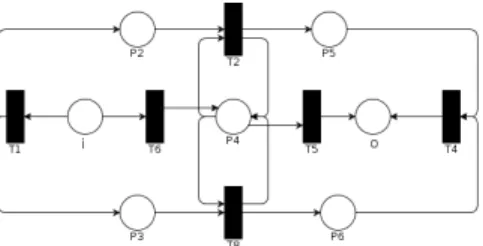
Fig. 2.Basic example of a WF-net (ex1)
As mentioned above, workflows can be modelled using a class of Petri nets, called the workflow nets (WF-nets). Figure 2 provides an example of a Petri net where the places are rep-resented by circles, the transitions by rectangles, and the arcs by arrows.
Definition 1 (Petri net). A Petri net is a tuple (P, T, F ) where P is a finite
set of places, T is a finite set of transitions (P ∩T = ∅), and F ⊆ (P ×T )∪(T ×P ) is a set of arcs.
Let g ∈ P ∪ T and G ⊆ P ∪ T . We use the following notations: g•= {g′|(g, g′) ∈
F},•g= {g′|(g′, g) ∈ F }, G•= ∪
g∈G g•, and•G= ∪g∈G •g.
A marking of Petri net is a function M : P →N. The marking represents the number of token(s) on each place. The marking of a Petri net evolves during its execution. Transitions change the marking of a Petri net according to the following firing rules. A transition t is enabled if and only if ∀p ∈•t, M(p) ≥ 1.
When an enabled transition t is fired, it consumes one token from each place of
•t and produces one token for each place of t•. With respect to these rules, a
transition t is dead at marking M if it is not enabled in any marking M′reachable from M . A transition t is live if it is not dead in any marking reachable from the initial marking. A Petri net system is live if each transition is live.
Definition 2 (WF-net). A Petri net P N = (P, T, F ) is a WF-net (Workflow
net) if and only if P N have two special places i and o, where•i= ∅ and o•= ∅,
and for each node n ∈ (P ∪ T ) there exists a path from i to o passing through n.
For example, the Petri net in Fig. 2 is a WF-net. Let us notice that in the context of workflow, specifiers are used to consider ordinary Petri nets [6], i.e. Petri nets with arcs of weight 1. In the rest of the paper, the following notations are used:
– M∅: the marking defined by ∀p ∈ P, M (p) = 0,
– Ma t
−
→ Mb: the transition t is enabled in marking Ma, and firing it results in
the marking Mb,
– Ma→ Mb: there exists t such that Ma t
− → Mb,
– M1 −→ Mσ n: the sequence of transitions σ = t1, t2, ..., tn−1 leads from the
marking M1to the marking Mn (i.e. M1−→ Mt1 2−→ ...t2 tn−1 −−−→ Mn),
– Ma ∗
−
→ Mb: the marking Mb is reachable from marking Ma (i.e. there exists
σsuch that Ma −→ Mσ b).
We denote Mi(k)the initial marking (i.e. Mi(n) = k if n = i, and 0 otherwise)
and Mo(k) the final marking (i.e. Mo(n) = k if n = o, and 0 otherwise). When
k is not specified, it equals 1. A sequence σ of transitions of a Petri net is an execution if there are Ma, Mb such that Ma
σ
WF-net is an execution σ such that Mi −→ Mσ o. For example, Mi −→ Mσ o where
σ = T 6,T 5 is a correct execution of the WF-net in Fig. 2. The behaviour of a WF-net is defined as the set Σ of all its correct executions. For the transition t and the execution σ, the function Ot(σ) is the number of occurrences of t in σ.
Definition 3 (Siphon/Trap). Let N ⊆ P such that N 6= ∅:
– N is a trap if and only if N•⊆ •N.
– N is a siphon if and only if•N ⊆ N•.
Figure 3(a) displays an example of a Petri net with a siphon. Let N = {P 4}, since•N= {T 1, T 8} ⊆ N•= {T 1, T 8}, the set of places N = {P 4} is a siphon.
Theorem 1 (from [7]). An ordinary Petri net without siphons is live. 3.2 WF-nets with Modalities
Modal specifications have been designed to allow loose specifications to be ex-pressed by imposing restrictions on transitions [5]. They allow specifiers to in-dicate that a transition is necessary or just admissible. In the framework of WF-nets, this concept provides two kinds of transitions: the must-transitions and the may-transitions. A may-transition (resp. must-transition) is a transi-tion fired by at least one executransi-tion (resp. all the executransi-tions) of the procedure modelled by a WF-net.
While basic modal specifications are useful, they usually lack expressiveness for real-life applications, as only individual transitions are concerned with. We propose to extend modal specifications to express requirements on several tran-sitions and on their causalities. To this end, the language S of well-formed modal specification formulae is inductively defined by : ∀t ∈ T, t is a well-formed modal formula, and given A1, A2 ∈ S, A1∧ A2, A1∨ A2, and ¬A1 are well-formed
modal formulae. These formulae allow specifiers to express modal properties
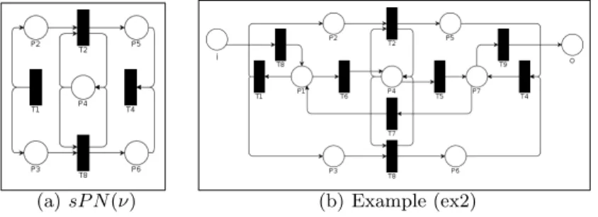
about WF-nets’ correct executions. Any modal specification formula m ∈ S can be interpreted as a may-formula or a must-formula. A may-formula describes a behaviour that has to be ensured by at least one correct execution of the WF-net. The set of may-formulae forms a subset of CTL formulae where only the possibly operator (i.e. along at least one path) is used. On the other hand, a must-formula describes a behaviour that has to be ensured by all the correct executions of the WF-net. The set of must-formulae forms a subset of CTL formulae where only the inevitably operator (i.e. along all paths) is used. For example, for the WF-net ex2 of 3(b), the may-formula T 9 means that there exists a correct execution firing transition T 9 at least once (i.e. T 9 is a may-transition). More complex be-haviours can be expressed. For example, the must-formula (T 8∧T 9)∧(¬T 6∨T 5) means that T 8 and T 9 must be fired by every correct execution, and if an exe-cution fires T 6 then T 5 is also fired at least once. Formally, given t ∈ T :
– P N |=may tif and only if ∃ σ ∈ Σ. Ot(σ) > 0, and
Further, given a well-formed may-formula (resp. must-formula) m ∈ S, a WF-net P N satisfies m, written P N |=may m (resp. P N |=must m), when at
least one (resp. all) correct execution(s) of P N satisfies (resp. satisfy) m. The semantics of ¬, ∨ and ∧ is standard.
Definition 4 (Modal Petri net). A modal Petri net M P N = (P, T, F, m, M )
is a Petri net P N = (P, T, F ) together with a modal specification (m, M ) where: – m ∈ S is a well-formed modal must-formula4, and
– M ⊂ S is a set of well-formed modal may-formulae.
We say that a WF-net P N satisfies a modal specification (m, M ) if and only if P N |=mustmand ∀m′ ∈ M, P N |=may m′.
3.3 Hierarchical Petri Nets
Modelling large and intricate WF-nets can be a difficult task. Fortunately, simi-larly to modular programming, WF-nets can be designed using other WF-nets as building blocks. One of the simple methods used to construct composed WF-nets is by transitions substitution. A composed WF-net built using this method has special transitions that represent several whole (composed or not) WF-nets. The composed WF-nets can then be viewed as WF-nets with multiple layers of details; they are called hierarchical WF-nets. While this does not add any expres-siveness to WF-nets, it greatly simplifies the modelling work, allowing to model small parts of the whole process that are combined into a composed WF-net. 3.4 Constraint System
A constraint system is defined by a set of constraints (properties), which must be satisfied by the solution of the problem it models. Such a system can be repre-sented as a Constraint Satisfaction Problem (CSP) [8]. It is such that each vari-able appearing in a constraint should take its value from its domain. Formally, a CSP is a tuple Ω =< X, D, C > where X is a set of variables {x1, . . . , xn}, D is
a set of domains {d1, . . . , dn}, where di is the domain associated with the
vari-able xi, and C is a set of constraints {c1(X1), . . . , cm(Xm)}, where a constraint
cj involves a subset Xj of the variables of X. A CSP thus models NP-complete
problems as search problems where the corresponding search space is the Carte-sian product space d1× . . . × dn. The solution of a CSP Ω is computed by a
labelling function L, which provides a set v (called valuation function) of tu-ples assigning each variable xi of X to one value from its domain di such that
all the constraints C are satisfied. More formally, v is consistent—or satisfies a constraint c(X) of C—if the projection of v on X is in c(X). If v satisfies all the constraints of C, then Ω is a consistent or satisfiable CSP. In the rest of the paper, the predicate SAT (C, v) is true if the corresponding CSP Ω is made satisfiable by v, and the predicate U N SAT (C) is true if there exists no such v.
4
We only need a single must-formula because P N |=mustm1∧ P N |=mustm2 if and
Using Logic Programming for solving a CSP has been investigated for many years, especially using Constraint Logic Programming over Finite Domains, writ-ten CLP(FD) [9]. This approach basically consists in embedding consiswrit-tency te-chniques into Logic Programming by extending the concept of logical variables to the one of the domain-variables taking their value in a finite discrete set of integers. In this paper, we propose to use CLP(FD) to solve the CSP that represent the modal specifications to be verified.
4
Verification of Modal Specifications
To verify a modal specification of a net, we model the executions of a WF-net by a constraint system, which is then solved to validate or invalidate the modal specifications of interest.
4.1 Modelling Executions of WF-nets
Considering a WF-net P N = (P, T, F ), we start by modelling all the executions leading from a marking Ma to a marking Mb, i.e. all σ such that Ma
σ
−→ Mb.
Definition 5 (Minimum places potential constraint system). Let P N = (P, T, F ) be a WF-net and Ma, Mb two markings of P N , the minimum places
potential constraint system ϕ(P N, Ma, Mb) associated with it is:
∀p ∈ P.ν(p) = X t∈p• ν(t) + Mb(p) = X t∈•p ν(t) + Ma(p) (1)
where ν : P × T →N is a valuation function.
Equation (1) expresses the fact that for each place, the number of token(s) entering it plus the number of token(s) in Ma is equal to the number of tokens
leaving it plus the number of token(s) in Mb. This constraint system is
equiva-lent with respect to solution space to the state equation, aka the fundamental equation, of Petri nets, the only difference is that (1) explicitly gives information about the places involved in the modelled execution.
Theorem 2. If Ma −→ M∗ b then a valuation satisfying ϕ(P N, Ma, Mb) exists.
Proof. Let σ = t1, t2, ..., tn and Ma −→ Mt1 1−→ Mt2 2...Mn−1−→ Mtn b. We define:
– ∀t ∈ T.ν(t) = Ot(σ) – ∀p ∈ P.ν(p) =Pj∈{1,2,...,n−1}∪{a,b}Mj(p) Then ∀p ∈ P : – Pj∈{1,2,...,n−1}∪{a,b}Mj(p) =Pt∈p•Ot(σ) + Mb(p) = P t∈•pOt(σ) + Ma(p). Indeed, as the WF-net is an ordinary Petri net, the sum of tokens in all markings of a place is equal to the sum of the occurrences of transitions producing (resp. consuming) a token at this place plus the number of token(s) in marking Mb (resp. Ma).
– ν(p) =Pt∈p•ν(t) + Mb(p) = P
t∈•pν(t) + Ma(p). Consequently, ν is a valuation satisfying ϕ(P N, Ma, Mb).
For example, Mi σ
−→ Mowhere σ = T 6, T 5 is a correct execution of the
WF-net in Fig. 2, therefore we can find a valuation ν(n) = 1 if n ∈ {T 6, T 5, i, o}, and ν(n) = 0 otherwise. By Th. 2, this valuation ν satisfies the constraints system ϕ(ex1, Mi, Mo).
Theorem 2 allows to conclude that a WF-net P N does not have any cor-rect executions if ϕ(P N, Mi, Mo) does not have a valuation satisfying it.
How-ever, even if there is a valuation satisfying ϕ(P N, Mi, Mo), it does not
neces-sary correspond to a correct execution. For example, the valuation ν(n) = 1 if n ∈ {T 1, T 2, T 8, T 4, i, P 2, P 3, P 5, P 6, o}, ν(n) = 2 if n ∈ {P 4}, and ν(n) = 0 otherwise, satisfies ϕ(ex1, Mi, Mo) but it does not correspond to any correct
execution. This is due to the fact that transitions T 2 and T 8 cannot fire si-multaneously using as an input token an output token of each other. Conse-quently, the set of solutions of ϕ(P N, Mi, Mo) constitutes an over-approximation
of the set of correct executions of P N . In the rest of the paper, the solutions of ϕ(P N, Mi, Mo) that do not correspond to correct executions of P N are called
spurious solutions. Hence our goal is to refine this over-approximation in order to be able to conclude on properties relative to all correct executions of a WF-net. 4.2 Verifying Structural Properties over Executions
While considering the modelling of WF-net executions, siphons and traps have interesting structural features. Indeed, an unmarked siphon will always be un-marked, and a marked trap will always be marked. Therefore a WF-net can only have siphons composed of at least the place i and traps composed of at least place o. Theorem 3 allows to conclude on the existence of a siphon in a WF-net. Theorem 3. Let θ(P N ) be the following constraint system associated with a
WF-net P N = (P, T, F ): – ∀p ∈ P, ∀t ∈•p.P
p′∈•tξ(p′) ≥ ξ(p)
– Pp∈Pξ(p) > 0
where ξ : P → {0, 1} is a valuation function. P N contains a siphon if and only if there is a valuation satisfying θ(P N ).
Proof. (⇐) Let ξ be a valuation satisfying θ(P N ), and N ⊆ P such that ξ(p) =
1 ⇔ p ∈ N . Then ∀p ∈ N, ∀t ∈•p.P
p′∈•tξ(p′) ≥ 1, which implies•N ⊆ N•.
Consequently, N is a siphon.
(⇒) Suppose that N is a siphon then obviously the valuation ξ(p) defined as: ξ(p) = 1 if p ∈ N , and 0 otherwise, satisfies θ(P N ).
For example, for the WF-net of Fig. 2 where the set of places N = {P 4} is a siphon, ξ(p) = 1 if p ∈ N, else 0 is a valuation satisfying θ(ex1).
The places (excluding places i and o) and transitions composing a correct execution of a WF-net cannot form a trap or a siphon. Using this propriety we refine the over-approximation made using ϕ(P N, Mi, Mo). Theorem 4 states that
for any solution of ϕ(P N, Ma, Mb), the subnet, composed of places (excluding
place i and o) and of the transitions of the modelled execution, contains a trap if and only if it has also a siphon. Therefore we only need to check the presence of a siphon (or, respectively, of a trap).
Theorem 4. Let P N = (P, T, F ) a WF-net, Ma, Mbtwo markings of P N , and
ν : P × T → N a valuation satisfying ϕ(P N, Ma, Mb). We define the subnet
sP N(ν) = (sP, sT, sF ) where:
– sP = {p ∈ P \ {i, o} | ν(p) > 0} – sT = {t ∈ T | ν(t) > 0}
– sF = {(a, b) ∈ F | a ∈ (sP ∪ sT ) ∧ b ∈ (sP ∪ sT )}
If sP N (ν) contains a trap (resp. siphon) N then N is also a siphon (resp. trap). Proof. (⇒) Let N ⊆ sP such that N 6= ∅, so Pp∈Nν(p) = Pp∈NPt∈p•ν(t) =Pp∈NPt∈•pν(t). It implies P p∈N P t∈p•∩N•ν(t) + P p∈N P t∈p•∩sT N•ν(t) = Pp∈NPt∈•p∩N•ν(t) + P p∈N P
t∈•p∩sT N•ν(t) that can be simplified as P p∈N P t∈p•ν(t) = P p∈N P t∈•p∩N•ν(t) + P p∈N P t∈•p∩sT N•ν(t) because ∀p ∈ N.p•∩ sT N• = ∅ . Let N be a trap (N• ⊆ •N) such that N is not
a siphon (•N * N•). Thus, one has P p∈N P t∈p•ν(t) = P p∈N P t∈•p∩N•ν(t) implyingPp∈NPt∈p•ν(t) = P p∈N P t∈p•ν(t) + P p∈N P t∈•p∩sT N•ν(t). We finally have ∀p ∈ N.•p∩ sT N• = ∅ because ∀t ∈ sT.ν(t) > 0. This implies •N ⊆ N•, a contradiction.
(⇐) The proof that if N is a siphon then N is a trap, is similar.
Theorem 5. The Petri net sP N (ν) contains no siphon and no trap if and only
if θ(sP N (ν)) does not have a valuation satisfying it. Proof. Follows from Th. 3 and 4.
Using Th. 5 allows defining the constraint system in Th. 6, which refines ϕ(P N, Ma, Mb). Thanks to this new system, the spurious solutions of ϕ(P N, Ma, Mb)
corresponding to an execution with siphon/trap are no more considered. Theorem 6. Let P N = (P, T, F ) be a WF-net and Ma, Mb two marking of
P N. There exists ν : P ×T →N a valuation satisfying ϕ(P N, Ma, Mb) such that
θ(sP N (ν)) does not have a satisfying valuation if and only if there exist σ and k∈N such that ∀p ∈ P \{i}. Ma′(p) = Ma(p), Ma′(i) = k, ∀p ∈ P \{o}.Mb′(p) = Mb(p), Mb′(o) = k, Ma′
σ
−→ Mb′ and ∀t ∈ T. Ot(σ) ≥ ν(t).
Proof. (⇒) Suppose ν : P × T → N is a valuation satisfying ϕ(P N, Ma, Mb)
such that θ(sP N (ν)) does not have a satisfying valuation. By Th. 5, sP N (ν) contains no siphon and therefore is live (cf. Th. 1). It implies that there is σ such that Ma −→ Mσ b in sP N (ν) where ∀t ∈ sT. Ot(σ) ≥ ν(t). Using the fact
that a transition of σ is in i•, and a transition of σ is in •o, we can conclude
that Ma′
σ
(⇐) Suppose σ such that Ma −→ Mσ b and ∀t ∈ T. Ot(σ) = ν(t). By Th. 2 we can
complete the definition of ν to make ν a satisfying valuation of ϕ(P N, Ma, Mb).
In addition, sP N (ν) contains no siphon and no trap because it would contradict Ma
σ
−→ Mb. By Th. 5, θ(sP N (ν)) does not have a satisfying valuation.
For example, let us consider the WF-net of Fig. 2, the valuation ν(n) = 1 if n ∈ {T 1, T 2, T 8, T 4, i, P 2, P 3, P 5, P 6, o}, ν(n) = 2 if n ∈ {P 4}, otherwise ν(n) = 0, is a satisfying valuation of ϕ(ex1, Mi, Mo). The set of places N = {P 4}
is a trap/siphon. Figure 3(a) displays sP N (ν). Therefore by Th. 3 there is a valuation satisfying θ(sP N (ν)). By Th. 6, ν does not correspond to a correct execution of the WF-net of Fig. 2.
(a) sP N (ν) (b) Example (ex2)
Fig. 3.WF-net examples used to illustrate over-approximation
The constraint system of Th. 6 can be used to over-approximate the correct executions of a WF-net. Indeed, for the WF-net in Fig. 3(b), the valuation ν(n) = 1 if n ∈ {T 1, T 8, T 6, T 2, T 7, T 8, T 5, T 9, T 4, i, P 2, P 3, P 5, P 6, o}, ν(n) = 2 if n∈ {P 1, P 7}, and ν(n) = 3 if n ∈ {P 4}, is a valuation satisfying ϕ(ex3, Mi, Mo)
such that θ(sP N (ν)) does not have a satisfying valuation. By Th. 6 there exist σ and k such that Mi(k)
σ
−→ Mo(k)and ∀t ∈ T. Ot(σ) ≥ ν(t).
In this case there is no σ such that k = 1. Indeed, P 4 cannot be empty when either T 2 or T 8 is fired, and therefore a marking with at least one token in P 4 and one in either P 2 or P 3 must be reachable. As there is no execution possible with only one token that leads to such marking, we have k > 1.
While defining an over-approximation might be useful for the verification of safety property, in our case, we want to be able to verify a modal specification. As the approximation is difficult to handle, we need to be able to model an execution that violates the modal specification if it exists.
Theorem 7. Let P N = (P, T, F ) be a WF-net, and Ma, Mbits two markings. If
there is ν : P ×T →N such that SAT (ϕ(P N, Ma, Mb), ν)∧U N SAT (θ(sP N (ν)))
∧∀n ∈ P × T. ν(n) ≤ 1 then Ma σ
−→ Mb and ∀t ∈ T. Ot(σ) = ν(t).
Proof. Any place is involved with at most one transition consuming one token,
and at most one transition producing one token. By Th. 6 one has Ma′
σ
−→ Mb′. Since at most one transition can consume a token in i (resp. produce a token in o), we have Ma′ = Ma (resp. Mb′ = Mb).
In the rest of the paper, a segment of an execution is defined as an execution modelled by the constraint system in Th. 7. In this way, we now propose to de-compose an execution modelled by the constraint system of Th. 6 into segment(s) modelled by Th. 7. If such a decomposition exists then the execution is a correct execution. Otherwise, we can conclude that the found solution is a spurious one. Indeed, spurious solutions can appear because the order of transition firing is not taken into account in the modelled execution. Therefore, decomposing the execution into segments forces the ordering of transitions where order matters. Theorem 8. Let P N = (P, T, F ) be a WF-net, and Ma, Mb its two markings.
Ma σ
−→ Mb if and only if there exists k ∈ N such that M1 σ1
−→ M2· · · Mk σ(k) −−→ Mk+1, where M1= Ma, Mk+1= Mb and for every i, 0 < i ≤ k, there is νi s.t.
SAT(ϕ(P N, Mi, Mi+1, νi)) ∧ U N SAT (θ(sP N (νi))) ∧ ∀n ∈ P × T. νi(n) ≤ 1.
Proof. (⇒) Suppose Ma −→ Mσ b where σ = t1, . . . , tk then by definition there
exist M1 −→ Mt1 2· · · Mk t(k)
−−→ Mk+1, where M1 = Ma, Mk+1 = Mb.
More-over, for every i, 0 < i ≤ k, there is νi such that SAT (ϕ(P N, Mi, Mi+1, νi)) ∧
U N SAT(θ(sP N (νi))) ∧ ∀n ∈ P × T. νi(n) ≤ 1, as νi is a valuation modelling
the execution of a single transition. (⇐) Follows from Th. 7.
In the rest of the paper, we denote φ(P N, Ma, Mb, k) the constraint system
of Th. 8, where k is the number of segments composing the execution. As φ(P N, Mi, Mo, k) can be used to model any execution of P N composed of k
or less segments, we propose to use it to determine the validity of a WF-net with regards to a given modal specification.
4.3 Verifying Modal formulae
When determining whether or not a WF-net satisfies the modal properties of in-terest, we distinguish two decision problems. The first one, called the K-bounded
validity of a modal formula, only considers executions formed by K segments,
at most. The second one, called the unbounded validity of a modal formula, deals with executions formed by an arbitrary number of segments; it general-izes the first problem. To verify modalities over a single transition, constraint systems come very naturally into the play. Intuitively, for a may-transition t, determining one correct execution firing t at least once is enough to validate its may-specification. On the other hand, for a must-transition t, the lack of correct executions without firing it validates its must-specification.
In our approach, verifying modal specifications from Def. 4 relies on their expression by constraints. To build these constraints, for every transition t ∈ T , the corresponding terminal symbol of the formulae is replaced by ν(t) > 0, where ν is the valuation of the constraint system. For example, for the modal formula (T 0 ∧ T 5) ∧ (¬T 7 ∨ T 6), the corresponding constraint is (ν(T 0) > 0 ∧ ν(T 5) > 0)∧(¬ν(T 7) > 0∨ν(T 6) > 0). Given a modal formula f ∈ S, C(f, ν) denotes the constraint built from f , where ν is a the valuation of the constraint system. The following theorem extends the constraint systems to verify modal specifications.
Theorem 9. Let M P N = (P, T, F, m, M ) a modal WF-net. The WF-net P N = (P, T, F ) satisfies the modal specification (m, M ) if and only if:
– there is no ν, k ∈N such that SAT (φ(P N, Mi, Mo, k) ∧ ¬C(m, ν), ν), and
– for every f ∈ M , there exist ν, k ∈ N such that SAT (φ(P N, Mi, Mo, k) ∧
C(f, ν), ν).
Proof. By Th. 8, there exist ν, k ∈N such that SAT (φ(P N, Mi, Mo, k) ∧ ¬C(m,
ν), ν) if and only if P N 2must m. In addition, there are ν, k ∈ N such that
SAT(φ(P N, Mi, Mo, k) ∧ C(f, ν), ν) if and only if P N |=mayf.
Theorem 9 can be adapted to the case of hierarchical WF-nets. In this case, the modal formula has to be verified for the main WF-net, i.e. the highest level net, and also for the WF-nets substituting transitions at lower levels.
Theorem 10. Let P N = (P, T, F ) be a WF-net, ¯Rmust the set of all
well-formed must-formulae not satisfied by P N , and Rmay the set of all well-formed
may-formulae satisfied by P N . There exists Kmax such that:
– ∀f ∈ ¯Rmust,∃ ν, k ≤ Kmax. SAT (φ(P N, Mi, Mo, k) ∧ ¬C(f, ν), ν),
– ∀f ∈ Rmay,∃ ν, k ≤ Kmax. SAT (φ(P N, Mi, Mo, k) ∧ C(f, ν), ν).
Proof. Sketch. The set of correct executions of a WF-net is possibly infinite.
This is due to the fact that T-invariants (i.e. sequence of transitions σ such that M −→ M ) could be fired indefinitely. However, when considering the verificationσ of modal formulae, we are only interested in the presence or absence of transitions in correct executions (i.e. the number of their firings does not matter). Therefore considering the set of correct executions where T-invariants are allowed to fire at most once is enough to check the validity of modal formulae. This restricted set of correct executions is finite. As a consequence, there exists Kmaxsuch that
any execution of this set can be modelled by Kmax segments, at most.
Theorem 10 implies that for any WF-net P N = (P, T, F ), there exists Kmax
such that any modal may-formula (resp. must-formula) f can be verified re-garding the consistency of the constraint system φ(P N, Mi, Mo, Kmax) ∧ C(f, ν)
(resp. φ(P N, Mi, Mo, Kmax) ∧ ¬C(f, ν)). In other words, to verify any
may-formula (resp. must-may-formula), it is not necessary to look for the existence (resp. non-existence) of correct execution respecting (resp. not respecting) the be-haviour expressed by the may-formula (resp. must-formula) of this WF-net com-posed of more than Kmax segments. However determining the Kmax value of a
WF-net from its structure is still an open problem. However, we can infer an upper-bound ofP|T |j=1j!.
5
Implementation and Experiments
The proposed approach has been fully automated, allowing practitioners, at any stage of the workflow design, to verify modal formulae using an integrated tool chain. This section describes this tool chain developed to experimentally validate the proposed approach, and illustrates its use and obtained results on the case study introduced in Sect. 2.
5.1 Implementation Architecture
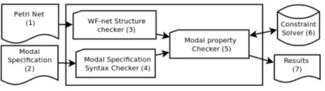
As a proof of concept, an implementation supporting the approach we propose has been developed to provide an integrated tool chain to design WF-nets and verify modal specifications. The architecture is shown in Fig. 4.
Fig. 4.Tool chain description
The tool chain takes as inputs a WF-net model (1) and the modal specifica-tions (2) to be verified. WF-net model is exported from a third party software (e.g., Yasper [10], PIPE [11]) as an XML file, as well as the modal specifications that are expressed in a dedicated and proprietary XML format. From these in-puts, the developed tool first checks the structure of the WF-net model (3) to exclude Petri nets that do not correspond to WF-nets definition (cf. Def. 2). It then checks the modal specifications regarding the syntax proposed in Sect. 4 (4). Once validated, these inputs are translated into a constraint system (5) that is handled using the CLP(FD) library of Sicstus Prolog [12] (6). Finally, a report about the validity of modal specifications of the WF-net is generated (7).
To verify a may-formula (resp. a must-formula) m (resp. M ), the tool first checks if there exists a solution of the over-approximation, given by Th. 6, such that the modelled execution satisfies (resp. does not satisfy) m (resp. M ). If such an execution exists, it then tries to find an execution of the under-approximation, given by Th. 8, which satisfies (resp. does not satisfy) m. As an illustration, Figure 5 gives the algorithm of the function checking the validity of a must-formula. It returns the K-bounded validity of a given modal formula m. To cope with the complexity raised by Kmax, K can be fixed to a manageable value.
Nevertheless, when fixing K to Kmax (or greater than Kmax), the algorithm
enables to decide the unbounded validity of the must-formula m. The results in Sect. 4.1 ensure its soundness and completeness. Finally, solving a CSP over a finite domain being an NP-complete problem with respect to the domain size, this algorithm inherits this complexity.
5.2 Experimental Results
The approach and the corresponding implementation have been firstly validated on a set of models collected from the literature, especially from [4, 13, 14], and afterwards experimented in the field of issue tracking systems using the industrial example described in Sect. 2. Table 1 shows an extract of the experimental results obtained on this industrial example, focusing on the six properties (p1to p6) and
Inputs:P N- a WF-net, m - a must-formula, K a positive integer. Results:T RU E- P N|=mustm, F ALSE - P N 2mustm.
function IsMustValid(P N ,m,K)
ifSAT(ϕ(P N, Mi, Mo)∧ ¬C(m, ν), ν) ∧ U N SAT (θ(sP N (ν))) then
k= max({v(n)|n ∈ T }) ifk== 1 then return F ALSE else
whilek≤ K do
if SAT(φ(P N, Mi, Mo, k)∧ ¬C(m, v), ν) then return F ALSE
else k= k + 1 end if end while returnT RU E end if else returnT RU E end if end function
Fig. 5.Algorithm checking the validity of a must-formula
The properties p1to p6are representative of the kind of properties that have
to be verified by engineers when they design the business process to be imple-mented. Moreover, These properties are sufficiently clear without a complete description of the workflow and enable to show all possible outcomes of our ap-proach. The modal formula associated with each property is specified, and the result of the computation is given by its final result as well as the internal evalu-ation of ϕ. The input K and the corresponding computed value of φ(K) are also precised when it makes sense, i.e. when the algorithm cannot conclude without this bound.
When verifying must-formulae that are satisfied by the WF-net (see p1, p2 and
p3), or may-formulae that are not satisfied by the WF-net (see p4), the
over-approximation proposed in Th. 6 is usually enough to conclude. On the other hand, when verifying may-formulae that are satisfied by the WF-net (see p5), or
must-formulae that are not satisfied by the WF-net (see p6), the decomposition
into K segments is needed. We empirically demonstrate that this decomposition is very effective since values of Kmaxare usually moderate (Kmax= 6 in the case
of p5, less than 10 with all the experimentations on this case-study). We can also
notice the definitive invalidity of p6 (a user can exit the current session without
logout), which enabled to highlight an ambiguity in the textual requirements. Thanks to the experiments, we can conclude that the proposed method is feasible and efficient. Moreover, the developed tool is able to conclude about the (in)validity of the studied properties in a very short time (less than a second).
# Formula ϕ K φ(K) Result
p1P N|=must(SubA∧ ¬SubA) ∨ (SubB ∧ ¬SubA) TRUE - - TRUE
p2P N|=mustSubB⇒ Login TRUE - - TRUE
p3P N|=mustSR CreateCRIT SIT⇒ (V andD ∨ U pdate ∨ Closure) TRUE - - TRUE
p4P N|=maySR CreateCRIT SIT⇒ (U pdate ∧ Closure) FALSE - - FALSE
p5P N|=maySR U pgradeT oCRIT SIT TRUE 1 FALSE FALSE6 TRUE TRUE
p6P N|=mustLogin⇒ Logout FALSE 1 FALSE FALSE
6
Conclusion and Related Work
Modal specifications introduced in [15] allow loose or partial specifications in a process algebraic framework. Since, modal specifications have been ported to Petri nets, as in [16]. In this work, a relation between generated modal languages is used for deciding specifications’ refinement and asynchronous composition. Instead of comparing modal languages, our approach deals with the correct exe-cutions of WF-nets modelled by constraint systems. A lot of work has been done [17–19] in order to model and to analyse the behaviour of Petri nets by us-ing equational approaches. Among popular resolution techniques, the constraint programming framework has been successfully used to analyse properties of Petri net [20, 21]. But, like in [21], the state equation together with a trap equation are used in order to verify properties such as deadlock-freedom. Our approach also takes advantage of trap and siphon properties in pursuance of modelling correct executions. Constraint programming has also been used to tackle the reacha-bility problem—one of central verification problems. Let us quote [22] where a decomposition into step sequences was modelled by a constraint system. Our approach is similar, the main difference is that the constraints we propose on step sequences, i.e. segments, are stronger. This is due to the fact that we are not only interested in the reachability of a marking, but also in the transitions involved in the sequences of transitions that reach it.
This paper hence presents an original and innovative formal framework based on constraint systems to model executions of WF-nets and their structural prop-erties, as well as to verify their modal specifications. It also reports on encoura-ging experimental results obtained using a proof-of-concept tool chain. In par-ticular, a business process example from the IT domain enables to successfully assess the reliability of our contributions. As a future work, we plan extensive experimentation to determine and improve the scalability of our verification ap-proach based on constraint systems. We also need to improve its readiness level in order to foster its use by business analysts. For instance, we could propose a user-friendly patterns to express the modal properties. Finally, generalizing our approach by handling coloured Petri nets is another research direction.
Acknowledgment
This project is performed in cooperation with the Labex ACTION program (contract ANR-11-LABX-0001-01) – see http://www.labex-action.fr/en.
References
1. van der Aalst, W.M.P., ter Hofstede, A.H.M.: YAWL: Yet Another Workflow Language. Journal of Information Systems 30(4) (June 2005) 245–275
2. Dumas, M., Hofstede, A.H.M.t.: UML Activity Diagrams As a Workflow Specifica-tion Language. In: Proc. of the 4th
Int. Conf. on The Unified Modeling Language (UML’01), Toronto, Canada, Springer-Verlag (October 2001) 76–90
3. van der Aalst, W.M.P.: The Application of Petri Nets to Workflow Management. Journal of Circuits, Systems, and Computers 8(1) (February 1998) 21–66 4. van der Aalst, W.M.P.: Three Good reasons for Using a Petri-net-based Workflow
Management System. Journal of Information and Process Integration in Enter-prises 428 (December 1997) 161–182
5. Larsen, K.G.: Modal Specifications. In: Proc. of the Int. Workshop on Automatic Verification Methods for Finite State Systems. Volume 407 of LNCS., Grenoble, France, Springer-Verlag (June 1989) 232–246
6. van der Aalst, W.M.P.: Verification of Workflow Nets. In: Proc. of the 18th
Int. Conf. on Application and Theory of Petri Nets (ICATPN’97). Volume 1248 of LNCS., Toulouse, France, Springer (June 1997) 407–426
7. Heiner, M., Gilbert, D., Donaldson, R.: Petri Nets for Systems and Synthetic Biology. In: Proc. of the 8th
Int. School on Formal Methods for Computational Systems Biology (SFM’08). Volume 5016 of LNCS., Springer (June 2008) 215–264 8. Macworth, A.K.: Consistency in networks of relations. Journal of Artificial
Intel-ligence 8(1) (1977) 99–118
9. Tsang, E.: Foundation of constraint satisfaction. Academic Press (1993)
10. van Hee, K., et al.: Yasper: a tool for workflow modeling and analysis. In: Proc. of the 6th
Int. Conf. on Application of Concurrency to System Design (ACSD’06), Turku, Finland, IEEE CS (June 2006) 279–282
11. Bonet, P., Llad´o, C.M., Puijaner, R., Knottenbelt, W.J.: PIPE v2.5: A Petri net tool for performance modelling. In: Proc. of the 23rd
Latin American Conference on Informatics (CLEI’07), San Jose, Costa Rica (October 2007)
12. Carlsson, M., et al.: SICStus Prolog user’s manual (Release 4.2.3), Swedish Insti-tute of Computer Science, Kista, Sweden. (October 2012)
13. Kouchnarenko, O., Sidorova, N., Trcka, N.: Petri Nets with May/Must Seman-tics. In: Proc. of the Workshop on Concurrency, Specification, and Programming (CS&P’09), Krak´ow-Przegorzaly, Poland (September 2009) 291–302
14. van der Aalst, W.M.P.: Business Process Management Demystified: A Tutorial on Models, Systems and Standards for Workflow Managemen. In: Lectures on Concurrency and Petri Nets. Volume 3098 of LNCS., Springer (2004) 1–65 15. Larsen, K.G., Thomsen, B.: A modal process logic. In: Proc. of the 3rd
Annual Symp. on Logic in Computer Science (LICS’88), IEEE (July 1988) 203–210 16. Elhog-Benzina, D., Haddad, S., Hennicker, R.: Refinement and asynchronous
com-position of modal petri nets. In: Transactions on Petri Nets and Other Models of Concurrency V. Volume 6900 of LNCS. Springer (2012) 96–120
17. Desel, J.: Basic linear algebraic techniques for place/transition nets. In: Lectures on Petri Nets I: Basic Models. Volume 1491 of LNCS. Springer (1998) 257–308 18. Wimmel, H., Wolf, K.: Applying CEGAR to the Petri Net State Equation. In:
Proc. of the 17th
Int. Conf. on Tools and Alg. for the Construction and Analysis of Systems (TACAS’11). Volume 6605 of LNCS., Springer (March 2011) 224–238 19. Schmidt, K.: Narrowing Petri Net State Spaces Using the State Equation.
Funda-menta Informaticae 47(3-4) (October 2001) 325–335
20. Soliman, S.: Finding minimal P/T-invariants as a CSP. In: Proc. of the 4th
Workshop on Constraint Based Methods for Bioinformatics (WCB’08). (May 2008) 21. Melzer, S., Esparza, J.: Checking system properties via integer programming. In:
Proc. of the 6th
Eur. Symp. on Programming Languages and Systems (ESOP’96). Volume 1058 of LNCS., Link¨oping, Sweden, Springer (April 1996) 250–264 22. Bourdeaud’huy, T., Hanafi, S., Yim, P.: Incremental Integer Linear Programming
Models for Petri Nets Reachability Problems. Petri Net: Theory and Applications (February 2008) 401–434