HAL Id: hal-00080377
https://hal.archives-ouvertes.fr/hal-00080377
Submitted on 21 Jan 2010HAL is a multi-disciplinary open access archive for the deposit and dissemination of sci-entific research documents, whether they are pub-lished or not. The documents may come from teaching and research institutions in France or abroad, or from public or private research centers.
L’archive ouverte pluridisciplinaire HAL, est destinée au dépôt et à la diffusion de documents scientifiques de niveau recherche, publiés ou non, émanant des établissements d’enseignement et de recherche français ou étrangers, des laboratoires publics ou privés.
Image Compression Using Subband Wavelet
Decomposition and DCT-based Quantization
Mahmoud Addouche, Fatma Zohra Nacer, Réda Yahiaoui
To cite this version:
Mahmoud Addouche, Fatma Zohra Nacer, Réda Yahiaoui. Image Compression Using Subband
Wavelet Decomposition and DCT-based Quantization. WSEAS Transactions on Signal Processing, 2006, 2 (4), pp.518-524. �hal-00080377�
Image Compression Using Subband Wavelet
Decomposition and DCT-based Quantization
Addouche M.†, Nacer F. Z.* and Yahiaoui R. † (†) Femto-ST Institute, LPMO Dept.,
32, avenue de l'observatoire - 25044 Besançon cedex, France. (*)Ecole Centrale d’Electronique, 53 rue de Grenelle 75007 Paris.
Abstract — The aim of this work is to evaluate the
performance of an image compression system based on wavelet-based subband decomposition. The compression method used in this paper differs from the classical procedure in the direction where the scalar quantization of the coarse scale approximation sub-image is replaced by a discrete cosine transform (DCT) based quantization. The images were decomposed using wavelet filters into a set of subbands with different resolutions corresponding to different frequency bands. The resulting high-frequency subbands were vector quantized according to the magnitude of their variances. The coarse scale approximation sub-image is quantized using scalar quantization and then using DCT-base quantization to show the benefit of this new optional method in term of CPU computationa1 cost vs restitution quality.
INTRODUCTION
Image compression consists in minimizing the volume of data needed for the image representation. The objective of image compression techniques is the reduction of the amount of bits required to represent an image, with or without the loss of information. Compression can be achieved by transforming the data, projecting it on a basis of functions, and then encoding the resulted coefficients. A common way to realize the encoding is to quantize the coefficients and apply some lossless compression such as Huffman on the quantized coefficients. Another way to compress an image is to use the subband coding method. This method splits the coefficients according to distinct levels of information description in order to quantize separately according to its own special properties and planned compression ratio for each level. The use of subband decomposition in data compression and coding is widely used in the image compression field [1]. The scalar or vector quantization (QV) are the typically quantization approach to achieve the encoding phase.
As they exhibit the orientation and frequency selectivity of images, the wavelets are considered as a powerful signal processing tool to exploit the affectivity of the subband image coding [2 to 4]. Applying the wavelet transform on images does not reduce the amount
of the data but it provides a representation of the image to be compressed which is more useful to be compressed. The possibility of compression by quantizing and encoding the wavelet coefficients relies on the assumption that details at high resolution are less visible to the eye and therefore can be eliminated or reconstructed with low-order precision.
The subband decomposition supplements the representation base transformation by allowing several abstraction levels. This decomposition is achieved using Mallat’s pyramidal multiresolution architecture [3]. After the image was decomposed, the wavelet coefficients giving the high-frequency coefficients were vector quantized whereas the low-frequency coefficients (approximation image) where generally scalar quantized.
The compression method, which is being used in this paper, differs from this classical procedure in the direction where the scalar quantization of the approximation image is replaced by a discrete cosine transform (DCT) based quantization.
A predetermined compression ratio to be used for each shape in the pyramidal structure is given, and different sizes and dimensions of codebook are tested. The results are given when using scalar quantization and also when the a DCT applied before encoding the low-frequency coefficients, in order to demonstrate that this technique enable much lower CPU computationa1 cost with similar quality and compression rate.
SUBBAND IMAGE DECOMPOSITION
BASED ON WAVELETS
Multiresolution analysis based on Wavelets is introduced by Meyer [5], Mallat [6], and Daubechies [7] in their construction of orthogonal wavelets. From then on, the multiresolution nature of the discrete wavelet transform is proven as a powerful tool to represent images decomposed long the vertical and horizontal directions using the pyramidal multiresolution scheme. Using this analysis, the image is decomposed with different resolutions into a set of subimages called shapes corresponding to different frequency bands.
Two-Channel Filter Banks
Consider the one-dimensional discrete signal Si(n)
shown in Fig. 1 where i denotes the resolution level. The Mallat’s pyramidal decomposition[3] decomposes the discrete approximation Si(n) into the approximation at a
coarser resolution Si+1(n) and the detail signal Di+1(n)
which corresponds to the difference of information between the resolution levels i and i+1. The lower resolution signal Si+1(n) is obtained by halfband lowpass
filtering Si(n) followed by downsampling by a factor of
two in order to make it fullband again. In a similar
fashion, the higher resolution signal Di+1(n) is the
downsampled version of the signal resulting from highpass filtering. The transfer functions fl(n) and fh(n)
correspond to the impulse responses of the lowpass and highpass filters used to realize the subbands decomposition for any resolution level.
Fig. 1. Basic two-channel filter bank structure.
As depicted in Fig. 1, the signal reconstitution is achieved by upsampling the signals and Di+1(n) through
insertion of zeros, followed by the application of the lowpass and highpass synthesis filters with their impulse responses gl(n) and gh(n); respectively.
Image Representation in the Wavelet Base
Multiresolution decomposition on k levels of a two-dimensional signal results into a set of 3k+1 subbands defining the DWT representation on k levels of the discretized image. As shown in Fig. 2, the two-dimensional wavelet analysis consists of successively applying the one-dimensional DWT, using a row-column approach.
Fig. 2. One level of subband image decomposition.
For a given 2n
x 2n image Si(n, m), wavelet
decomposition is performed by convolving the rows of this image with the one-dimensional impulse responses fl
and fh before repeating this operation according to the
vertical direction on the obtained two subbands. Because of the downsampling with a factor of two, we obtain at a given resolution level, four shapes from the two-dimentional decomposition of one approximation shape. The final size of each of these shapes is 2n-1x 2n-1.
Subband Si+1 contains the smooth information and the
background intensity of the image and the subbands
Dx
i+1; Dyi+1; and Dyxi+1 contain the detail information of
the image. The subband Si+1 corresponds to the lowest
frequencies, Dx
i+1 gives the horizontal high frequencies,
Dy
i+1 gives the vertical high frequencies, and Dyxi+1 the
high frequencies in both directions.
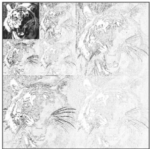
Fig. 3. Two levels of subband decomposition of 512 x 512 image.
Fig. 3 shows a two-level wavelet decomposition scheme for a 512 x 512 digital image. At the first level of
the decomposition, we obtain 256 x 256 subbands; three
shapes representing vertical, horizontal, and diagonal edges; and an approximation shape which is decomposed at the second level, in a same fashion, into four smaller
shapes (128 x 128 subimages). As Fig. 3 depicted it,
representing the wavelet coefficients produced by a
k-level decomposition needs as many pixels as the
original image contains.
To compute an exact reconstruction of the original image, one uses the two dimension extension of the algorithm described in the section above (see Fig. 1). At each step, the image Si is reconstructed from Si+1, Dxi+1,
Dyi+1, and Dyxi+1. Between each column of the i+1th
resolution shapes, we add a column of zeros, convolve the rows with a one dimensional filter, add a row of zeros between each row of the resulting image, and convolve the columns with another one-dimensional filter. For details, refer to [3]. fl y ↓ 2 fh y ↓ 2 fl x ↓ 2 Si fl y ↓ 2 fh y ↓ 2 fh x ↓ 2 Si+1 xy i
D
+1 x iD
+1 y iD
+1 fl(n) Si(n) Si(n) fh(n) ↓2 i+1(n) S g ↑2 l(n) gh(n) ↓2 ↑2 Di+1(n)STATISTICAL PROPERTIES OF THE
WAVELET COEFFICIENTS
In this section, we show how to use the sensitivity of the human visual system as well as the statistical properties of the image to optimize the coding by the wavelet representation. This section is dedicated to determine the appropriate quantization factors for each resolution level and shape.
Statistical Properties
The probability density function (PDF) is frequently used to parameterize the quantization method in each subband [11]. Fig. 4 shows the highband coefficient PDF
of a 512 x 512 image (Fig. 3) for level 2 and both
decomposition directions.
Fig. 4. The probability density function (PDF) of the highband Wavelet coefficients (horizontal,
vertical and both direction).
Examining lots of gray-level’s portrait images shows that the distribution of the wavelet coefficients remains similar for all the shapes at the same level or at different levels, excluding the "approximation" subband. From the distribution of the highband wavelet coefficients, it can be seen that most of the coefficients lie in a narrow range around the origin.
Table. 1. Wavelet coefficient variance for several resolution levels, according to each direction.
Level Shape Lenna Apple Cluster 1 x 33.00 3.43 1.14 1 y 11.97 5.31 2.12 1 xy 7.95 0.54 0.05 2 x 42.94 7.01 3.50 2 y 20.77 10.30 4.18 2 xy 12.08 2.51 0.75 3 x 95.34 11.89 11.10 3 y 71.20 28.08 16.43 3 xy 24.64 5.61 3.33 4 x 141.74 22.63 31.37 4 y 143.47 67.39 45.05 4 xy 57.81 13.96 9.78
Another way to judge the importance of the information contained in each subband is to estimate the dispersion magnitude of the wavelet coefficients. Table. 1. contains the variance values calculated for three
example images, according to each decomposition direction and various resolution levels.
One can see from Table. 1 that the variance of diagonal decomposition is lower than the horizontal and vertical decompositions. In addition, the variances decrease with the increasing of resolution level. Estimating energy distribution and dispersion magnitude of the wavelet coefficients makes it possible to better design an appropriate quantization strategy.
VECTOR QUANTIZATION OF WAVELET
COEFFICIENTS
Vector Quantization (VQ) [9] has been widely known for its excellent rate-distortion performance in the lossy data compression field. Several approaches have been reported for image coding by VQ of transform coefficients rather than the image pixels [10-11] and are referred to as transform vector quantization (TVQ).
Principle of VQ
The objective of vector quantization is to build a set of N vectors Yi (i = 1 to N) called Codebook, allowing an
optimal description of the n vectors Xj (j = 1 to n) which
compose the image to be vector quantized. This quantization method is a form of pattern recognition or matching where an input pattern is approximated by one standard template of a predetermined codebook. The
Linde, Busu and Gray (LBG) algorithm [8] is frequently
used to perform codebook design for image compression. This technique is an iterative method which involves creating a letter reference to indicate which of the
codebook vector Yi is nearest to each subimage (or
vector) Xj. This letter reference is refined step by step to
converge towards an optimal alphabet which allows the weakest error between the original shape and the reconstructed one. The encoding and decoding scheme in Fig 5 demonstrates the use of VQ.
Fig. 5. Vector quantization encoding and decoding scheme
In case of the multiresolution decomposition, it is more judicious to group and train together the vectors in each shape according to each subband properties. As shown before, the statistical properties are contrasted
with the subband direction and the resolution level. Therefore, the LBG algorithm is used with additional rules that take into the count the statistical properties of each shape when designing the codebooks.
Subband Codebook Design
As the VQ encoding consists in approximating the sequence to be encoded by a vector belonging to the codebook, the design of this last one is an essential process in image compression approaches combining wavelet decomposition and vector quantization. Considering the preceding results, wavelet coefficients have to be coded hierarchically according to their location (in the sense of pyramidal level and texture shape) in order to optimize the quality of the final reconstructed image; thus, the designed codebooks are also called subband codebooks. We use this quantization method only for the subbands containing detail informations. The sizes of vectors and codebooks are chosen according to the suspected quantization impact on the quality of the reconstructed image. We chose to perform a dyadic progression of the codebook and vector sizes according to the resolution level and texture shape. Thus, the codebook size (number of template vectors) decreased with the increasing of the resolution level and the vectors of the diagonal shapes are larger than those of the lateral shapes. These rules are formulated below (Eq. 1): NvL(s) = NvL(st) SHR [sNvL · (si-s)] NvD(s) = NvD(st) SHR [sNvD · (st-s)] KxL(s) = KxL(st) SHL [skL · (st-s)] KyL(s) = KyL(st) SHL [skL · (st-s)] KxD(s) = KxD(st) SHL [skD · (st-s)] KyD(s) = KyD(st) SHL [skD · (st-s)] (1) where
NvL(s): Vector count for a lateral shape at level s.
NvD(s): Vector count for a diagonal shape at level s.
sNvL: Dyadic step of the lateral vector count.
sNvD: Dyadic step of the diagonal vector count.
skL: Dyadic step of the lateral vector dimensions.
skD: Dyadic step of the diagonal vector dimensions.
st: Target resolution level.
KxL(s), KyL(s): Vector dimensions for a lateral shape at
level s.
KxD(s), KyD(s): Vector dimensions for a diagonal shape
at level s.
num SHL cnt: Multiply num by 2, cnt times num SHR cnt: Divide num by 2, cnt times
According to these rules, the size of the vectors increase with a factor of 4sKL (or (2×2)sKL) while their count
decreases with a factor of 2sNvL (L is indicative of the lateral shapes; replace L by D for the diagonal shapes). As
to case where the vector count is null, the shapes will not be coded and thus, no codebook is designed.
Two parameters relating to the compression ratio have to be defined; the codebook size which depends on the number and size of its vectors and the size of the partition (liste of the references to the codebook vectors in place of the original vectors of the image) which depends on the shape dimension and codebook size.
Let τ(s), T(s), and ρ(s) be, respectively, the ratio compression between shape and its partition, the shape dimension in pixels and the codebook size; s is the resolution level. We can thus give:
(2) s
s
T
s
T
=
⋅
−2⋅ 0)
2
(
)
(
)
(
)
(
2
)
0
(
8
)
(
)
(
)
(
)
(
(2 3)s
K
s
B
T
s
B
s
K
s
T
s
s⋅
=
⋅
=
− +τ
(3))
(
)
(
)
(
s
=
K
s
⋅
Nv
s
ρ
(4) with K(s) = Kx(s)·Ky(s) Kx(s) = Kx(st) SHL [sk · (st-s)] Ky(s) = Ky(st) SHL [sk · (st-s)] Nv(s) = Nv(st) SHR [sNv · (st-s)] Nv(s) = Nv(st) SHR [sNv · (st-s)] (5)The factor of 8 is due to the use of 256 gray levels for the image color representation. s0 is the initial resolution
level; thus, T(s0) is the size in pixels of the image to be
compressed. Nv(s) is the number of vectors in the codebook at the resolution level s. Bit count we need for indexing Nv(s) codebook vectors is given by B(s). The dimension in pixels of each codebook vector at the resolution level s is given by K(s). Variables sNv and sk correspond, respectively, to sNvD and skD for diagonal
shapes and sNvL and skL for lateral shapes.
Thus, one can deduce, according the target resolution level st, the compression ratio relating to the partitions
and the size of codebooks as follows:
(6)
)
(
)
(
2
2
1 2i
i
L s i D s SBVQ t tτ
τ
τ
=
+
∑
+
= ⋅ − (7)( ) ( )
( ) ( )
∑
=+
=
st i D D L L SBVQK
i
Nv
i
K
i
Nv
i
12
ρ
QUANTIZATION OF THE LOW-PASS
BAND COEFFICIENTS
The sensitivity of the final reconstructed image quality to the quantization errors is more noticeable at lower levels (approximation shape), which necessitates
higher reconstruction quality. The lowband wavelet coefficients can be quantized using lossless data compression algorithms like Huffman coding [13] or LZW (Lempel-Ziv-Welch) [14]. However, the real need to obtain increasingly high compression ratios led us to seek methods of compression of the lowband image which would bring only one low distortion relative to the compression ratio profit. Scalar quantization (SQ), among other lossy compression methods, gives us rather appreciable results [11-12]. SQ corresponds to the particular case where codebook vector length is reduced to 1. We actually noted only one weak degradation compared to the improvement of the ratio compression but we also noticed a considerable disadvantage of the Scalar Quantization which is the slowness of its execution. Since the approximated image (lowband shape) has the same statistical and psychovisual properties as that of an ordinary image, we tested a DCT-based quantization method.
DCT-based Image Quantization
The discrete cosine transform (DCT) helps separate the image into parts (or spectral sub-bands) of differing importance (with respect to the image's visual quality). This allows for lossy compression of image data by determining which information can be thrown away without too much compromising the image. The DCT is used in many compression and transmission codecs, such as JPEG and MPEG [15-16]. Pixel loss is due to the "zig-zag" sequence used to balancing the quantization of the DCT coefficients and not to DCT transform. When the classical DCT-based compression method leads to arrange the coefficients according to that weight decreasing sequence, our method affects the same weight to the whole coefficients. The reason is that the few of detail information remaining in the lowband coefficients, after a strong compression, must be preserved as well as possible.
The DCT coefficients we obtained are gathered into vectors of the same frequency band in order to have a well balanced quantization. To achieve the compression, each of the 8×8 DCT coefficients is uniformly quantized in conjunction with a 64-element quantization table (refer to [18] for details). The bit allocation needed to code this table is given in Equ. 8:
⎟⎟ ⎠ ⎞ ⎜⎜ ⎝ ⎛ + ⋅ = float Q I T L B B B 64 2 (8)
where BT is the bit allocation we need to code the
64-element quantization table, BI is the image size in bits,
Bfloat is the number of bits allowing to code a float and LQ
is the quantization level count of DCT coefficient.
EXPERIMENTAL RESULTS
The resulting images were evaluated by the peak signal to noise ratio (PSNR), defined as
(
)
∑∑
= = − = W i H j ij ij a a WH PSNR 1 1 2 2 10 ˆ 1 255 log 0 1 (9)where 255 is the peak gray level of the image, aij and
âij are the pixel gray levels from the original and
reconstructed images, respectively, and W×H is the total number of pixels in the image.
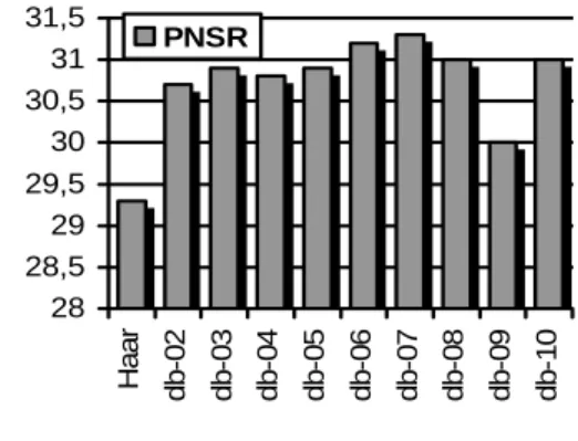
Fig. 6 represents the peak signal to noise ratio obtained when reconstruct LENNA image from its second level decomposition. All the wavelet coefficients that correspond to the detail information are replaced by zero. This preliminary test allows us to identify the filter potentially giving the best reconstitution quality. According to the figure above, the filter which is used for the following experiments is the 7th order Daubechies
filter [7]. 28 28,5 29 29,5 30 30,5 31 31,5 Haar db-02 db-03 db-04 db-05 db-06 db-07 db-08 db-09 db-10 PNSR
Fig. 6. PSNR of LENNA image reconstitution for various types of filters when all highband shapes
are discarded
The aim of an image compression is to reduce data size while keeping a good enough quality of the image restitution. Thus, we need to appreciate the relation binding the compression rate we can obtain for the various parameter setting.
Table. 2. PSNR of LENNA image reconstitution according to vector count and dimensions.
Initial Vector count : Nv(0)=
KL(2), KD(2) 2 4 8 16 32 64 128 256 2x2 . 2x2 31.7 32.4 33 33.9 34.7 35.6 36.5 37.6 2x2 . 4x4 31.7 32.4 32.9 33.7 34.5 35.4 36.4 37.8 4x4 . 4x4 31.5 31.8 32.1 32.6 33.5 34.7 36.8 42.3 4x4 . 8x8 31.5 31.8 32.2 32.7 33.7 35.1 37.1 42.3 8x8 . 8x8 31.5 31.7 32.3 33.3 36.3 42.3 8x8 . 16x16 31.4 31.7 32.3 33.6 36.6 42.3
The aim of an image compression is to reduce data size while keeping a good enough quality of the image restitution. Thus, we need to appreciate the relation
binding the compression rate we can obtain for the various parameter setting. Table. 2, and Table. 3, show the PSNR and the compression ration, respectively, we obtain for various number and dimensions of the codebook vectors. The compression ratio is expressed in the form of equivalent Bit per pixel (BPP).
256 128 64 32 16 8 4 2 8x8, 16x16 8x8, 8x8 4x4, 8x8 4x4, 4x4 2x2, 4x4 2x2, 2x2 30 32 34 36 38 40 42 44
Fig 7. PSNR of LENNA image reconstitution according to vector count and dimensions
Fig. 7 shows that the PSNR increases with the increase in the number of initial codebook vectors. The curve tends towards a line for low values of the vector sizes and towards an exponential curve for higher vector sizes.
Table. 3. BPP of a 256x256 image reconstitution according to vector count and dimensions.
Initial Vector count : Nv(0)=
KL(2), KD(2) 2 4 8 16 32 64 128 256 2x2 . 2x2 0.588 0.677 0.777 0.898 1.062 1.312 1.734 2.5 2x2 . 4x4 0.58 0.66 0.753 0.875 1.05 1.335 1.839 2.781 4x4 . 4x4 0.562 0.625 0.73 0.921 1.285 1.992 3.386 6.156 4x4 . 8x8 0.571 0.642 0.768 1.003 1.458 2.349 4.116 7.632 8x8 . 8x8 0.676 0.853 1.202 1.894 3.274 6.029 8x8 . 16x16 0.723 0.946 1.387 2.266 4.02 7.524 256 128 64 32 16 8 4 2 8x8, 16x16 8x8, 8x8 4x4, 8x8 4x4, 4x4 2x2, 4x4 2x2, 2x2 0 1 2 3 4 5 6 7
Fig. 8. BPP of a 256x256 image reconstitution according to vector count and dimensions.
Fig. 8 shows that the curve of the total number of bits by pixels (the codebook are taken into account) according to the initial vector number takes an
exponential form with an increase of the base according to the growth of the vector sizes. The exponential form is due to the space allocated to codebook. Thus, the curves will tend towards lines when the image size increases.
30 32 34 36 38 40 42 44 0 1 2 3 4 5 6 7 8 SBQV SBQV+DCTQ SBQV+SQ
Fig. 9. PSNR of LENNA in function of BPP when only suband vector quantization is performed,
when DCT quantization (DCTQ) is used in addition, and when SQ is use in place of DCTQ.
Fig. 9 depicts the PSNR we obtain in three cases: when only the suband vector quantization (SBVQ) is performed and the lowband image is preserved unchanged, when in addition of the SBVQ, a scalar quantization (SQ) is accomplished, and finally, when a DCT-based quantization is used in place of the SQ. Whole of these techniques are achieved for compression ratios varying from 37% to 95%. The PSNR when using DCTQ is globally little bit lower then those obtains performing a SQ for the lowband shape.
0 2 4 6 8 10 12 14 0 1 2 3 4 5 6 7 8 SBQV+DCTQ SBQV+SQ
Fig. 10. CPU computationa1 time according to the quantization method (DCTQ or SQ) used for the
lowband image.
Fig. 10, shows saving of time that one obtains using the DCT-based quantization. We notice that even gained CPU computational time is not linear, it is always positive. Compared with the SBVQ-SQ method, the DCT-based quantization of wavelet coefficients performed equally well or even better quality restitution with improved CPU computational time.
CONCLUSION
In this paper, we have developed an image coding scheme combining, in the wavelet domain, the subband vector quantization and a DCT-based quantization for image compression.
REFERENCES
[1] P. C. Cosman, R. M. Gray, and M. Vetterli, "Vector quantization of image subbands: A survey" IEEE Trans. Image Processing, vol. 5, pp. 202–225, 1996. [2] M. Antonini, M. Barlaud, P. Mathieu, and I.
Daubechies, "Image coding using wavelet transform", IEEE Trans. Image Processing, vol. 1, pp. 205–220, 1992.
[3] S. G. Mallat, "A theory for multiresolution signal decomposition: The wavelet representation", IEEE Trans. Pattern Anal. Machine Intell., vol. 11, pp. 674–693, 1989.
[4] S. G. Mallat, "Multifrequency channel decompo-sition of images and wavelet models" IEEE Trans. Acoust., Speech, Signal Processing, vol. 37, pp. 2091–2110, 1989.
[5] Y. Meyer, "Wavelets and operators" in Analysis at Urbana Z, Proc. of the Special Year in Modern Analysis at the Univ. of Illinois, 1986-1987, London Mathematical Society Lecture Notes Series, vol. 137. New York: Cambridge Univ. Press, pp. 256-365, 1989.
[6] S. Mallat, "Multiresolution approximation and wavelet orthonormal bases of L2(R)" Trans. Amer.
Math. Soc., vol. 315, pp. 69-81, 1989.
[7] I. Daubechies, "Orthonormal basis of compactly supported wavelets" Commun. Pure Appl. Math., vol. 41, pp. 909-996, 1988.
[8] Y. Linde, A. Buzo, and R. M. Gray, "An Algorithm for Vector Quantizer Design". Trans. IEEE Commun., Vol. COM-28, pp. 84-95, 1980.
[9] A.Gersho and R.M Gray, "Vector quantization and signal compression", Kluwer Academic Publishers, 1992.
[10] P. C. Cosman, R. M. Gray, and M. Vetterli, "Vector quantization of image subbands: a survey". Trans. IEEE Image Proc., Vol. 5, No. 2, pp. 202-225, 1996.
[11] A. Averbuch, D. Lazar, and M. Israeli, "Image compression using wavelet transform and multireslution decomposition". Trans. IEEE Image Proc., vol. 5, pp. 4-15, 1996.
[12] J. Max, "Quantizing for minimum distortion", IEEE Trans. Inform. Theory, vol. IT-6, Mar. 1960. [13] D.A. Huffman, "A method for the construction of
minimum-redundancy codes", Proceedings of the I.R.E., sep. 1952, pp. 1098-1102.
[14] T.A.Welch, "A technique for high-performance data compression." Computer. Vol. 17, pp. 8-19. June 1984.
[15] K. R. Rao and P. Yip, "Discrete Cosine Transform: Algorithms, Advantages, Applications". New York: Academic, 1990.
[16] J. Makhoul, "A fast cosine transform in one and two dimensions" IEEE Trans. Acoust. Speech Sig. Proc. 28 (1), 27-34 (1980).
[17] Y. Arai, T. Agui, M. Nakajima: "A fast DCT-SQ Scheme for Images", Trans IEICE #71 (1988), 1095-1097.
[18] F. Harris, D. Wright, "The JPEG Algorithm for Image Compression: A Software Implementation and some Test Results" Signals, Systems and Computers. Conference Record 24 Asilomar Conference on Volume 2, Issue , 5-7 Nov 1990 Page(s):870.