A linear height-resolving windfield model for tropical cyclone boundary layer

A Linear Height-Resolving Wind Field Model for

1

Tropical Cyclone Boundary Layer

2

Reda Snaiki, Teng Wu

*

3

Department of Civil, Structural and Environmental Engineering, University at Buffalo, State

4

University of New York, Buffalo, NY 14126, USA

5

*_{Corresponding author. Email: tengwu@buffalo.edu}

6

Abstract: The wind field model is one of the most important components for the tropical cyclone hazard 7

assessment, thus the appropriate design of this element is extremely important. While solving the fully non-8

linear governing equations of the wind field was demonstrated to be quite challenging, the linear models 9

showed great promise delivering a simple solution with good approximation to the wind field, and can be 10

readily adopted for engineering applications. For instance it can be implemented in the Monte Carlo 11

technique for rapid tropical-cyclone risk assessment. This study aims to develop a height-resolving, linear 12

analytical model of the boundary layer winds in a moving tropical cyclone. The wind velocity is expressed 13

as the summation of two components, namely gradient wind in the free atmosphere and frictional 14

component near the ground surface. The gradient wind was derived straightforwardly, while the frictional 15

component was obtained based on the scale analysis of the fully non-linear Navier-Stokes equations. The 16

variation of wind field with respect to the angular coordinate was highlighted since its contribution to the 17

surface wind speed and associated spatial distribution cannot be ignored in the first-order approximation. 18

The results generated by the present model are consistent with tropical cyclone observations. 19

Key words: Height-resolving wind-field model, Boundary layer, Scale analysis, Tropical cyclone. 20

21 22

1. Introduction

23

Tropical cyclone-related natural hazards are well known for resulting in the largest contribution to

24

insured losses each year. High winds in the tropical cyclone boundary layer cause widespread

25

damage to life and property in coastal areas. This situation has become more challenging due to

26

the changing climate and increasing coastal population density. A mature tropical cyclone typically

27

consists of four dynamically distinct parts, namely a boundary layer, a region above the boundary

28

layer (almost no radial motion), an updraft region, and a quiescent eye (Carrier et al. 1971). For

29

many engineering applications, only the boundary layer is concerned. Furthermore, in the

30

consideration of wind-induced damages, the dynamics of boundary layer, where the density

31

changes could be ignored, and the thermodynamics are usually independently examined, or weakly

32

coupled.

33

The dynamics of tropical cyclone boundary layer is essentially governed by the

Navier-34

Stokes equations of incompressible flow. The solution of dynamically coupled, intensively

35

interactive pressure and velocity fields is extremely challenging. In most of wind field models for

36

engineering applications, the pressure field (steady pressure gradient) is usually prescribed, either

37

based on the gradient wind equation (e.g., Shapiro 1983) or resulting from an empirical formula

38

(e.g., Schloemer 1954; Holland 1980). The wind speed could be simulated based on a slab

(depth-39

averaged) or height-resolving model. The slab wind field model has been widely applied to storm

40

surge modeling (e.g., Hubbert et al. 1991; Kennedy et al. 2012) and hurricane damage and loss

41

estimation (e.g., Florida Hurricane Loss Projection Model and HAZUS-MH Hurricane Model)

42

(Powell et al. 2005; Vickery et al. 2006) since the pioneering work of Chow (1971), Shapiro

43

(1983), and Thompson and Cardone (1996). However, there are several inherent limitations of the

44

slab model due to the vertical averaging of dynamic quantities in the boundary layer, as

comprehensively discussed by several studies (e.g., Kepert 2010a; 2010b). Among a series of

46

shortcomings, considering the boundary layer height as a constant and obtaining the near surface

47

winds based on empirical-based reduction factors may have considerable impact on the simulation

48

fidelity. Recently, Khare et al. (2009) has shown the linear height-resolving model is superior to

49

the slab model of tropical cyclone boundary layer based on the observation data of over-ocean

50

surface wind field.

51

The height-resolving model was originally derived by studying the tropical cyclone

52

boundary layer as a generalized Ekman problem (Haurwitz 1935; 1936; Rosenthal 1962). Later,

53

Yoshizumi (1968) integrated the storm movement into the model to account for the left-right

54

asymmetry of tropical cyclone wind field. On the other hand, Meng (1995; 1997) obtained similar

55

height-resolving solutions of boundary layer winds by carrying out perturbation analysis of the

56

Navier-Stokes equations. A so-called equivalent roughness length was introduced in Meng’s

57

model (1995; 1997) to simultaneously take the terrain roughness and topographical effects into

58

account, whereas the estimation of the equivalent roughness length for each case is not

59

straightforward. It should be noted that the abovementioned height-resolving models are actually

60

linear solutions. The state-of-the-art tropical cyclone risk assessment is essentially based on the

61

analysis framework established by Russell (1971), where the Monte Carlo sampling method is

62

utilized. This indicates a large number of simulations of the tropical cyclone boundary layer wind

63

filed are usually needed. Although nonlinear effects may not be always insignificant especially for

64

local flows (Kepert 2001; Kepert and Wang 2001), it is believed that the linear height-resolving

65

wind field model is a reasonable choice for many engineering applications (including risk

66

assessment) due to its high simulation efficiency.

In this study, the linear height-resolving wind field model was extracted based on the scale

68

analysis of the Navier-Stokes equations. The analytical expressions for wind speed components of

69

the tropical cyclone boundary layer were derived since they could facilitate the interpretation of

70

underlying physics. The obtained linear governing equations for boundary layer wind field are

71

different from those of previously widely-discussed models (Meng et al. 1995; Kepert 2001). For

72

example, several new terms that account for the contributions from the azimuthal variation of

73

velocity components are retained. It was demonstrated that the modification of surface wind speed

74

and its spatial distribution resulting from these new terms cannot be ignored. The new linear

75

height-resolving wind field model was validated using the observation data obtained during a

76

typhoon and a hurricane, respectively. Compared with Meng’s simulation, the new proposed

77

model shows improved representation of the wind field in the tropical cyclone boundary layer.

78

2. Boundary Layer Wind Model

79

In the boundary layer of a tropical cyclone, the horizontal momentum equations are typically

80

solved with a prescribed pressure distribution and a constant air density. Thus, the governing

81

equation of the wind field of a tropical cyclone is:

82 1 . p f t   _{       }  v v v k v F (1) 83

where v= wind velocity; t= time; f = Coriolis parameter; k = unit vector in the vertical direction;

84

= air density; F = frictional force; and p = Holland pressure expressed as:

85





exp - / B c m pp  p _ r r _ (2) 86

where pc= central pressure;  = central pressure difference; p rm= radius of maximum winds; r =

87

radial distance from the tropical cyclone center; and B = Holland’s radial pressure parameter. It

should be noted that bold character denote a vector. Eq. (1) is supplemented by the continuity 89 equation: 90 . d dt _{   v} (3) 91

which becomes for an incompressible flow:

92

. 0

 v (4)

93

To solve the governing equation of motion, the wind velocity (v) is expressed as the

94

summation of the gradient wind in the free atmosphere (v ) and the frictional component near the _g

95 ground surface (v'): 96  _g v v v' (5) 97

Consequently two separate equations can be derived:

98 1 . p f t           g g g g v v v k v (6a) 99 . . . f t  _{        }     g g    v' _{v v v v v v k v F} (6b) 100

Similar to Meng et al. (1995), the gradient wind pattern v is assumed to move in the free _g

101

atmosphere, at the translation velocity of the tropical cyclone c, thus the unsteady term can be

102 expressed as: . t      g g v

c v . On the other hand, the unsteady term t 

 v'

is significantly smaller than

103

the turbulent viscosity and inertia terms in the tropical cyclone boundary layer, and hence

104

neglected.

105 106 107

2.1 Gradient wind velocity

108

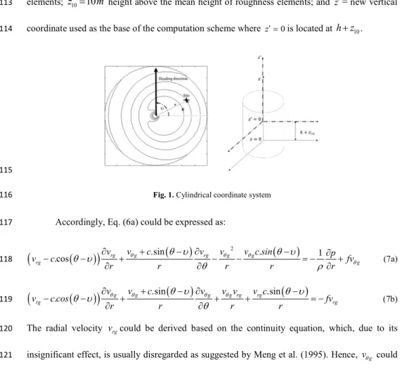
The cylindrical coordinate system ( , , )r z whose origin is located at the center of the tropical

109

cyclone is used to solve the governing equations. Fig. 1 illustrates the necessary parameters needed

110

for the present study, where= approach angle (counterclockwise positive from the East); =

111

azimuthal angle (counterclockwise positive from the East); h = mean height of the roughness

112

elements; z1010 m height above the mean height of roughness elements; and z = new vertical

113

coordinate used as the base of the computation scheme where z0is located at h z 10.

114

115

Fig. 1. Cylindrical coordinate system

116

Accordingly, Eq. (6a) could be expressed as:

117









.sin





2 .





1 .cos rg g rg g g rg g v v c v v v c sin p v c fv r r r r r                              (7a) 118







.



g g .sin





g g rg rg .sin





rg rg v v c v v v v c v c cos fv r r r r                          (7b) 119

The radial velocity v could be derived based on the continuity equation, which, due to its _rg

120

insignificant effect, is usually disregarded as suggested by Meng et al. (1995). Hence, vg could

121

be derived from Eq. (7a) as:

















₂ 1/2 2 4 g csin fr csin fr r p v r               _           (8) 123

The solution of gradient wind velocity is straightforward and was discussed in detail by several

124

researchers (e.g. Georgiou 1986; Meng et al. 1995).

125

2.2 Frictional wind velocity

126

The absolute angular velocity and vertical component of absolute vorticity of the gradient wind

127

are introduced first and given respectively by the following formulas (Meng et al. 1995):

128 2 g g v f r     (9a) 129 g g ag v v f r r        (9b) 130

As a result, Eq. (6b) in the cylindrical coordinate becomes:

131 2 2 2 1 ₂ g g v v u u u v v u w v K u u r r z r r  _     _  _  _{ }      _  _  _             (10a) 132 2 2 1 ' g g 2 ag v v v v v v u v v u u w u K v v r r z r r r  _        _  _ _  _{  }       _  _             (10b) 133

where ( , , )u v w = velocity vector; and , u v  are the frictional components of the wind velocity. The

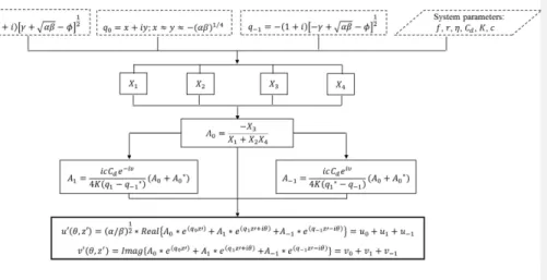
134

right hand side of Eqs. (10a) and (10b) represents the radial and azimuthal frictional force

135

components, respectively. The turbulent diffusivity K is assumed to be constant in this study.

136

The continuity equation can be expressed in the cylindrical coordinates as:

137

 

1 1 0 ru v w r r r  z  _  _ _    (11) 138

Then the vertical component of the wind velocity can be derived:

0 0 1 z 1 z w r udz vdz r r r          _{ } _{ }  _



_  _



_ (12) 140

Solving Eqs. (10a) and (10b) analytically is extremely difficult. In this study, they will be first

141

simplified using the scale analysis approach.

142

2.3 Scale analysis

143

In this section the same notation used by Vogl and Smith (2009) will be adopted for denoting the

144

scales of various quantities in Eqs. (10a) and (10b), as showed in Table 1:

145

Table 1. Scales of various quantities

146

Quantity u v vg v w r z g ag Change inp

Scale U  V  Vg V W R Z   p

147

Six non-dimensional parameters were introduced in Vogl and Smith (2009), namely Reynolds

148

number ReVZ K/ ; local Rossby numbers RoΛV/

 

RΛ and RoΞV/

 

RΞ ; Swirl

149

parameters Su'U V/ andSv' V V/ ; and A Z R / that is the aspect ratio of the boundary-layer

150

depth to the radial scale. It should be noted that based on the continuity equation namely Eq. (11),

151

the following result is obtained U R W Z/ ~ / .

152

The scale analysis for Eqs. (10a) and (10b) is presented in Tables 2 and 3, respectively. The

non-153

dimensional form is obtained by multiplying Eqs. (10a) and (10b) by 1/ 'ΞV and 1/ ' ΛU ,

154

respectively. It is worth mentioning that the terms 2K u₂

r    and 2 2 K v r   

 are not included in

155

Tables 2 and 3 since they have the same scale order as 2 2 h u K u r _{ }      and 2 2 h v K v r _{ }     , 156 respectively. 157

Table 2. Scale analysis of Eq. (10a)

158

Quantity Scale Normalized form

u u r     U2/R 2 1 U V S S Ro    g v v u r        (Vg V)_U R    SV1S RoU  u w z    WU/Z 2 1 U V S S Ro    2 v r   V2/R S RoV  gv    ΞV  ₁ 2 2 h u K u r _{ }      2 / KU R A R S



e V



1S RoU    2 2 u K z    2 / KU Z



AR Se V



1S RoU     159

Table 3. Scale analysis of Eq. (10b)

160

Quantity Scale Normalized form

v u r     U V /R S RoV Λ g v v v r        (Vg V V) R    S SV U 1RoΛ    v w z    WV/Z S RoV' Λ u v r   U V /R S Ro_{V Λ} agu   ΛU 1 g v v r      VV R  S S_{V U}1Ro_Λ 2 2 h v K v r _{ }      2 / KV R A R S



_{e U}



1Ro_Λ 2 2 v K z    2 / KV Z



AR Se U



1S RoV Λ    161

Typical values for the boundary layer such as the boundary layer height and the turbulent

162

diffusivity K were considered to assess the magnitude of each term. As a result, a new set of

163

equations could be obtained:

2 2 2 g g v v u u u v u u w v K r r z r z  _        _  _  _  _{ }         (13a) 165 2 2 g g ag v v v v v v u v v v u w u K r r z r r z  _       _                     (13b) 166

Solving the above nonlinear equations is demonstrated quite expensive. For engineering purposes,

167

the nonlinear equations could be simplified by linearization techniques.

168

3. Linear height-resolving model

169

3.1 Governing equations

170

Equations (13a) and (13b) could be linearized as:

171 2 2 g g v u _{v K} u r z  _   _{ }      (14a) 172 2 2 g g ag v v _u v v _K v r r z  _       _  _        (14b) 173

To solve the above-mentioned governing equations, the boundary conditions at the upper

174

atmosphere (15a) and above the ground surface (15b) need to be respectively employed:

175 ' 0 z v' (15a) 176 0 d z K C z      _  s s v' _{v v} (15b) 177

where v'= frictional component of the wind velocity; v_s= total wind velocity near the ground

178

surface; and Cd= drag coefficient.

179

New variables are introduced to simplify the solution namely: 1

2_K g   ; 1 2_K ag   ; 180 1 2 g v K r    ; and 1 2 g v Kr     

 . In addition, the variable



used in Kepert (2001) is employed:

u iv       (16) 182

It should be noted that the equations to be solved in this study are different from those in Kepert

183

(2001). Specifically, the equations have an additional term v vg

r





 

 since the gradient wind velocity

184

is considered to be dependent not only on the radial coordinate but the azimuthal one as well.

185

Furthermore, the translational velocity is integrated into the gradient wind velocity based on the

186

assumption that the wind pattern v moves at the translation velocity of the tropical cyclone c, g

187

while Kepert (2001) assumed a symmetric case of the gradient wind. Finally, the absolute angular

188

velocity g and vertical component of absolute vorticity of the gradient wind ag are exhibiting

189

not only a radial variation but and azimuthal one as well. Accordingly, Eqs. (14a) and (14b) could

190 be expressed as: 191

 

2 2 2 2i 2 Im 0 z         _{ } _{ }   (17) 192

 

Im  can be written as _i



_{  }*



_{2 (where} * _{indicates a complex conjugate), then Eq. (17)} 193 becomes: 194





2 * 2 2 i 2 i 0 z           _{   } _   (18) 195

The corresponding boundary condition expressed by Eq. (15b) could be decomposed using the

196

cylindrical coordinates into:

197



 

2



2 ' _{( ' ) ' '} d rg g rg u K C u v v v v u z         (19a) 198



 

2



2 ( ) d rg g g v K C u v v v v v z              (19b) 199

Eqs. (19a) and (19b) can be linearized considering , u v   v_g, hence, the final system to be solved 200 becomes: 201





2 * 2 2 i 2 i 0 z           _{   } _   (20a) 202

 









 





. 0 d g rg 0 K Re  C v v Re  (20b) 203

 









 





. 0 d g g 2 0 K Im  C v v  Im  (20c) 204 3.2 Analytical solutions 205

To solve system (20),



is expanded as Fourier series in azimuth, i.e.,



,



 

ik

k k z a z e       



 206

where a z is a complex coefficient (Kepert 2001). Then Eq. (20a) becomes: k

 

207



_{2 2}



 

 

*

 

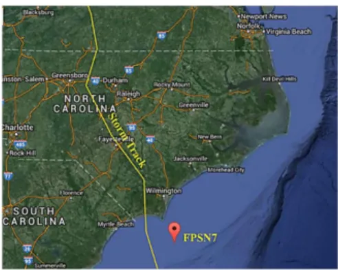
ik ₀ k k k k i k   a z a z i a z e       _{   }  _      



(21) 208

The complex coefficient ak can be expressed as a zk

 

 Akexp



q zk 



, and hence the following

209

equation could be obtained:

210

2 _{2 2} *

k k k k

A q i k   A i A  (22)

211

Since the wavenumbers higher than unity are not excited for a linear model, only the cases of

212

1

k  , k0, and k1 need to be considered.

213

Substituting



expression into Eqs. (20b) and (20c) leads to:

214 0 d g ik k k k C v Re A q e K            _ _         



 (23a) 215

2 2 0 d g ik d g k k k C v C v Im A q e i K K             _{ } _   



   (23b) 216

After a series of manipulations, one could obtain the frictional velocity components uand v(see

217

detailed derivation in Appendix A). Fig. 2 presents a step-by-step procedure in the development

218

of solutions for the proposed wind field model, where X1, X2, X3, X4 and  are five parameters

219

defined, respectively, as follows:

220









2 2 2 2 1 0 2 * 2 * 1 1 1 1 2 4 4 d d d d C c C c C fr X q C K K K q q K q q                   (24a) 221









2 2 2 2 * 2 0 2 * 2 * 1 1 1 1 2 4 4 d d d d C c C c C fr X q C K K K q q K q q                    (24b) 222 2 3 2 2 d iC fr X K      _  _   (24c) 223 * 4 0 ₂ d d 0 ₂ d d C C fr fr X q C q C K K K K          _  _{ }   _     (24d) 224









₂ 1/ 2 4 csin fr r p r      _{   }           (24e) 225

226

Fig. 2. u and v components of wind field model

227

As it can be seen from Fig. 2, u





,z



and v





,z



were decomposed respectively into three

228

components, i.e., u





,z   



u0 u u1 1 and v





,z   



v0 v v1 1. These components (i.e., u0,

229

0

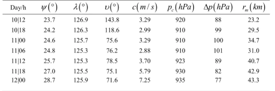
v, u1, v1, u1, v1) determine the direction and amplitude of the resultant frictional velocity.

230

While the real and imaginary components of q0 are approximated as:

 

1/4

x  y  as indicated

231

in Fig. 2, their exact solutions could be obtained based on Eqs. (A.19) and (A.20) (See Appendix

232

A for detailed derivation). The investigation of each component (i.e., u0, v0, u1, v1, u1, v1) will

233

be discussed in section 4.1.

234

4. Improved Representation

235

In this section, the spatial distribution of wind in the tropical cyclone boundary layer will be

236

investigated first based on a case study. Then two wind field models previously discussed by

237

researchers, namely Kepert’s model (2001) and Meng’s model (1995), will be explored to

238

demonstrate the advantages of the proposed linear height-resolving model in this study.

239 240

4.1 Spatial Distribution of the tropical cyclone wind field

241

To investigate the tropical cyclone spatial distribution, a case study is analyzed using the following

242

parameters:  p 60 hpa; rm80 km; c15 m s;



 90 C; Latitude 32.8 ; Longitude 243

129.7

 ;B ; 1 z00.1 m; 𝐾 = 100 𝑚 /𝑠; and  1.2 N s m2 4.

244

Figures (3a) and (3b) depict the contours of the gradient wind velocity and its

three-245

dimensional shaded surface, respectively. It can be concluded that the maximum wind speed is

246

located at rm and the difference of the maximum wind velocity between the right-hand side and

247

left-hand side is almost equal to the translational hurricane velocity c. Figures (3c) and (3d)

248

illustrate the contours of the surface wind velocity at the height around 10 m and its

three-249

dimensional shaded surface, respectively. The maximum wind speed is located on the right rear

250

quadrant for this specific case. The exact location of the maximum wind speed depends on a

251

number of factors such as the translation of the storm and the surface friction. Recently, Li and

252

Hong (2014) inspected the location of the maximum wind speed based on the H*Wind data where 253

totally 489 snapshots from 45 hurricanes, occurred during 2002 to 2013 were utilized. The H*Wind 254

was essentially developed by the Hurricane Research Division of the National Oceanic and

255

Atmospheric Administration (NOAA). It integrates several sources of wind data such as aircraft

256

reconnaissance, buoys, surface and remote sensing observations (Powell et al. 1998). To ensure

257

quality control, collected data are post-processed. The H*Wind database provides maximum

1-258

min sustained surface wind speed corresponding to a marine or open terrain over land exposures.

259

It is found that the maximum wind speed for 84% of the snapshots was located on the right side of

260

the storm motion. More specifically, 58% of these snapshots present the maximum wind speed at

261

the right rear quadrant and 42% at the right front quadrant.

263

Fig. 3. Spatial distribution of the wind speed: (a) Contour of the gradient wind speed; (b) three-dimensional shaded

264

surface of the gradient wind speed; (c) Contour of the surface wind speed at z around 10m; (d) three-dimensional

265

shaded surface of the surface wind speed

266

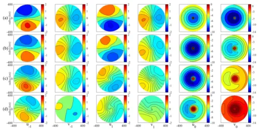
Figure (4) shows the u₀, v0, u1, v1, u1, and v1terms in the frictional component of the

267

boundary layer wind velocity using the same tropical cyclone data as in Fig. (3). Several

268

conclusions related to the behavior of u0, v0, u1, v1, u1, and v1 terms, can be drawn. First, it is

269

obvious that all frictional velocity components decay with height. Second, while u1 and v1 rotate

270

counterclockwise u₁ and v1 rotate clockwise. This behavior can be attributed to the signs of the

271

imaginary parts related to z and  in the complex exponential argument (i.e., _eq z i1 _and

272

q z i1 ₎

e   _{where opposite signs results in a counterclockwise rotation and vise-versa. Finally, due}

273

to the asymmetry of the tropical cyclone wind field, the proposed model allows the vertical length

scale for the depth of the boundary layer to exhibit not only radial variation but azimuthal one as

275

well, which is not the case for Kepert’s model (2001) where it varies only radially. The depth scale

276

related to (u0,v0), (u1,v1) and (u1,v1) are

 

1 4 0 1    , 12 1 1   _   _ and 277 1 2 1 1

  _    _ , respectively. For instance, 0 is a function of 𝛼 and 𝛽 which are

278

proportional to the absolute angular velocity and vertical component of absolute vorticity of the

279

gradient wind, respectively ( 1

2_K g    and 2 ) 1 ag K

   . These two variables are varying

280

radially and azimuthally due to the asymmetric structure of a moving tropical cyclone, therefore

281

0

 exhibits an asymmetric distribution. Since the rotational rate of each frictional component with

282

height is dependent on the corresponding depth scale, it can be concluded from the comparison of

283

1

 and 1that (u1,v1) rotates faster than (u1,v1), as indicated in the simulation results of Fig. 4.

284

285

Fig. 4. Frictional component of the boundary layer wind velocity u0, v0, u1, v1, u1, and v1 at z’=10m

286

(a); z’=200m (b); z’=500m (c); and z’=1000m (d)

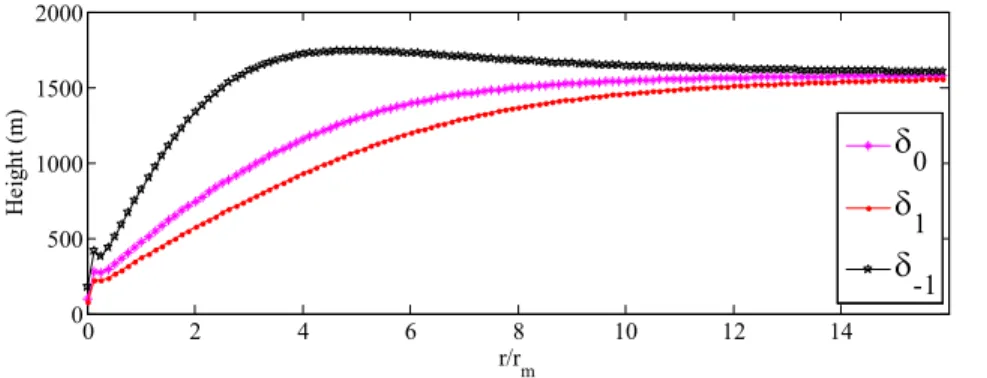
Figure 5 depicts the radial variation of the three depth scales 0, 1, 1. It can be

288

concluded that for larger radii all depth scales reduce to the classical Ekman height scale (namely

289

2K f



 ), where the Rossby number that measures the magnitude of the acceleration

290

compared to the Coriolis force is sufficiently small (𝑅𝑜 ≪ 1) (Ro 1). On the other hand, the

291

boundary layer depth decreases toward the center of the tropical cyclone (large Rossby numbers)

292

due to the effects of the storm rotation that results in predominated inertial and centrifugal forces,

293

as highlighted by several researchers (e.g., Rosenthal 1962; Kepert 2001). The results shown in

294

Fig. 5 are consistent with several numerical simulations and observations conducted by several

295

researchers (e.g., Kepert 2001; Kepert and Wang 2001) where the boundary layer depth varies

296

from a few hundred meters near from the inner core of the tropical cyclone to 1-3 km at larger

297

radii. Table 4 depicts the azimuthal variation of the depth scale for all frictional components.

298

Clearly, all depth scales depend on the azimuthal coordinate and thus should be taken into

299

consideration to enhance the simulation of the real behavior of a moving tropical cyclone.

300

301

Fig. 5. Radial variation of the depth scale of the boundary layer

302 303 0 2 4 6 8 10 12 14 0 500 1000 1500 2000 r/r_m H ei gh t ( m )



0



1



-1

Table 4.Boundary layer depth scale at r r _m (using the same tropical cyclone data of section 4.1) 304 ( )



 0( )m 1( )m 1( )m 0 477.2 369.7 826.0 30 482.3 367.4 769.2 60 496.4 374.1 749.0 90 516.2 388.1 761.5 120 536.3 406.0 800.6 150 551.3 423.1 858.9 180 556.7 434.6 929.1 210 551.3 437.4 1002.7 240 536.3 430.6 1062.0 270 516.2 415.9 1073.7 300 496.4 397.4 1015.0 330 482.3 380.4 916.0 360 477.2 369.7 826.0 305

4.2 Stationary tropical cyclone

306

For a stationary tropical cyclone, the translational velocity c , and hence0 A₁A₁0. 307

Accordingly, the frictional wind velocity components are degenerated into

308



 



1









2 _{0 0}

, * *exp

u  z    Real A q z and v



,z



Imag A{ *exp0



q z0 



} with

309



 

1/4

0 1

q   i  . It can be demonstrated in the stationary case that:

310

  

14



1 2 1 D g C X i v K      (25a) 311

   

14 2 2 1 D g C X i v K     (25b) 312 2 3 2 D g iC X v K   (25c) 313

  

14



  

14



4 1 D g 1 D g C C X i v i v K K        _   _{ }   _     (25d) 314

It should be noted that v_g was replaced by v since the gradient wind is symmetric for a stationary g

315

tropical cyclone. In Kepert (2001) a parameter X is defined as C v_{D g} K

 

 14. Then A₀ of a

316

stationary tropical cyclone could be expressed in terms of X as:

317





0 2 1 1 2 3 2 g X i X v A X X           (26) 318

The expression is exactly the same with that of Kepert (2001). This indicates that the specific case

319

of the stationary tropical cyclone in the proposed model provides the same solution in Kepert

320

(2001). This observation is expected since the gradient wind velocity for the case of a stationary

321

tropical cyclone is symmetric, which was an essential assumption in Kepert (2001).

322

4.3 Comparison with Meng’s model

323

The wind field model in Meng et al. (1995) is a special case of the present study. More specifically,

324

the contribution associated with u1, u1, v1, v1 and



was disregarded by Meng et al. (1995).

325

Accordingly, suppose u1u1 v1 v1  0, one has (see Appendix B for detailed derivation):

326













 









 

1 2 2 2 1 , cos sin 1 1 1 1 g g z v v u _ z _{ } e    _z    _z                        (27a) 327













2

 





2

 

1 , cos sin 1 1 1 1 g g z v v v _ z e    _z   _z                       (27b) 328 where d d 2 2 s s rs C C v v v K K        329

The solution developed by Meng et al. (1995) has similar form:

330

 

 

2 1 * cos sin z u_{ }e _D _z_{ }D _z_{ }   (28a) 331

 

 

( ) 1 2 *[ cos sin ] z v e_  D

_

z_{ }D

_

z_ (28b) 332 where









2 1 1 g 1 1 D    v_   ;





2 2 g 1 1 D v_   ; and



 



12_{. Consequently, it} 333

is shown that Meng’s model (1995) can be derived from the proposed model under the

above-334

mentioned assumptions. By comparison between Eqs. (27a) and (28a), it is noted that there is an

335

error in Meng’s original model, where the coefficient



should be replaced by 1/



. This

336

modification of the wind speed due to this error may not be negligible, as will be illustrated in the

337

validation example.

338

5. Validation

339

To validate the new tropical cyclone wind field model, wind records from hurricane Fran (1996)

340

and typhoon Maemi T0314 (2003) are used.

341

5.1 Hurricane Fran

342

Fran was one of the worst hurricanes ever to be recorded in North Carolina. It has reached

343

hurricane status on 29th _{August 29}th_{, 1996 and was registered as a Category 3 storm. Hurricane}

344

Fran made landfall on September 5th_{, 1996 on the North Carolina coast with an estimated central}

345

pressure of 954 hpa and a maximum sustained surface winds of 50 /m s . It created flooding in

346

the Carolinas, Virginia, West Virginia and Pennsylvania. Severe damage due to strong wind were

347

also recorded. Fran weakened to a tropical storm status over central North Carolina. Figure 6

348

depicts the location of the anemometer with respect to the storm track.

349

350

Fig. 6. Track of hurricane Fran and anemometer location

351

5.1.1 Hurricane Parameters

352

The necessary parameters for the simulation were recorded by the marine station FPSN7 from

353

September 5th _{to September 6}th_{. The station ID is 41013, located at (N33.44°,W77.74°). The} 354

National Hurricane Center’s North Atlantic hurricane database (HURDAT) (Jarvinen et al. 1984)

355

is the primary source of data. Typically, the parameters needed for the simulation are:



approach

356

angle; c translation velocity of the hurricane; pc central pressure; p central pressure difference;

357

m

r radius of maximum winds;  latitude; and  longitude. The parameter rm can be estimated

358

using several sources in the literature (e.g., Powell et al. 1991; 1998). This information is

359

supplemented by the H*Wind snapshots. There are several methods available in the literature to

360

estimate the parameter B (e.g., Vickery et al. 2000a; Holland 2008). For hurricane Fran the value

361

used was B0.95, which is the same value calculated by Vickery et al. (2000b). The period from

362

September 5th _{to September 6}th _{has known very strong winds from hurricane Fran especially in the} 363

eyewall region. Actually, the central pressure reached 952 hpa at 0600 UTC September 5th _in 364

which the hurricane center was located at (N29.8°,W76.7°) and slightly increased to reach

954 hpa at 0000 UTC September 6th _{where the hurricane center was located at (N33.7°,W78.0°)} 366

with a maximum sustained surface winds of 55 m/s.

367

5.1.2 Hurricane Simulation

368

The observed wind speeds and directions have been compared with those obtained by the proposed

369

wind field model. It should be noted that all parameters are obtained from the 6-hour interval track

370

information provided by the HURDAT database. The results generated by the present model are

371

consistent with hurricane observations as depicted in the Fig. 7.

372

373

374

Fig. 7. Observed and simulated wind speeds (top) and directions (bottom) of Hurricane Fran

375

5.2 Typhoon Maemi

376

Typhoon Maemi T0314 had devastating impacts on Japan and South Korea. It was born as tropical

377

depression near Guam on September 5th_{, 2003. Later, it was evolved into a typhoon on the} 378

September 7th _{of September and then intensified to reach a Category 5 typhoon storm reaching} 379

with a central pressure of 910 hpa . Maemi made landfall on September 12, 2003 on the south coast

380 6 12 18 24 0 10 20 30 40 50 Time (hour) W in d sp ee d (m /s )

Observed wind speed Simulated wind speed

6 12 18 24 0 90 180 270 360 Time (hour) W in d di re ct io n (° )

Observed wind direction Simulated wind direction

of the Korean peninsula and lasted approximately 6 hours in the South Korea leading to extensive

381

damage from wind, torrential rainfall and flooding. Wind records from typhoon Maemi will be

382

employed to highlight the difference between the results generated by the present model and

383

Meng’s model.

384

5.2.1 Typhoon Parameters

385

The observation point is located at the observatory of Miyako Island in Okinawa prefecture

386

(N24.8, E125.3 ). All the other necessary parameters for the typhoon simulation are obtained

387

from Yoshida et al. (2008), and listed in Table 5 for completeness:

388

Table 5. Typhoon Maemi parameters, September 2003 (Yoshida et al., 2008)

389

Day/h



 





 





 

 c m s



/



p hPa_c





p hPa





r km_m

 

10|12 23.7 126.9 143.8 3.29 920 88 23.2 10|18 24.2 126.3 118.6 2.99 910 99 29.5 11|00 24.6 125.7 75.6 3.29 910 100 34.7 11|06 24.8 125.3 76.2 2.88 910 101 31.0 11|12 25.7 125.3 78.5 3.70 923 89 40.7 11|18 27.0 125.5 75.1 5.79 930 82 42.9 12|00 28.7 125.9 71.6 7.25 935 77 43.3 390 5.2.2 Typhoon Simulation 391

The observed wind speeds and directions have been compared with those obtained by the proposed

392

wind field model. In addition, simulation results of the original and modified Meng’s models are

393

presented. As shown in Fig. 8, the results generated by the present model are consistent with the

394

typhoon observations.

396

397

Fig. 8. Observed and simulated wind speeds (top) and directions (bottom) of typhoon Maemi

398

To further inspect the results, a comparison of wind speeds and directions between results

399

obtained from the observed data and using the present and Meng’s models are presented in Fig. 9.

400

The corresponding correlation coefficients between the observations and various simulations for

401

wind speed and direction are calculated and presented in Table 6.

402 403 404 (10th) 120 18 (11th) 0 6 12 18 24 5 10 15 20 25 30 35 40 Time (hour) W in d sp ee d (m /s ) Measured data Proposed Model Original Meng Model Modified Meng Model

(10th) 120 18 (11th) 0 6 12 18 24 90 180 270 360 Time (hour) W in d di re ct io n (° ) Measured data Proposed Model Original Meng Model Modified Meng Model

0 10 20 30 40 0 10 20 30 40

Observed Wind Speed (m/s)

P re di ct ed W in d S pe ed ( m /s ) Observation Proposed Model Original Meng Model Modified Meng Model

0 90 180 270 360 0 90 180 270 360

Observed Wind Direction (°)

P re di ct ed W in d D ir ec ti on ( °) Observation Proposed Model Original Meng Model Modified Meng Model

405

Table 6. Correlation Coefficients of wind speed and direction

406

407

The results demonstrate that the wind velocities predicted by various models all match reasonably

408

well with the measured data, whereas the proposed model is superior to Meng’s model.

409 410

5.3 Vertical wind speed profile

411

Vertical wind speed profiles given by the proposed model, original and modified Meng’s models,

412

are plotted in Fig. 10 using the same tropical data of section 4.1. The location of the presented

413

wind speed profiles is selected at a distance equal to radius of maximum wind from the tropical

414

cyclone center and at zero degree from the East. The simulated wind profiles are normalized by

415

the gradient wind speed.

416

417

Fig. 10. Vertical profile of wind speed at r r _m

418 0.1 0.5 1 10 100 1000 2000

Wind speed/gradient wind speed

z'

(m

)

Proposed Model Original Meng Model Modified Meng Model

Model Wind speed Wind direction

Proposed Model 0.973 0.998

Meng’s model (original) 0.916 0.997

As it can be remarked from Fig. 10, the surface wind speed is underestimated by Meng’s

419

model compared to the proposed one. Same conclusion could be also obtained from the simulation

420

results in Fig. 8. Another interesting feature in the vertical wind speed profile of tropical cyclones

421

is the presence of a super-gradient-wind region, where the tangential winds are larger than the

422

gradient wind. A possible mechanism of this region was discussed by Kepert and Wang (2001),

423

where the super-gradient winds are attributed to the strong inward advection of angular

424

momentum. It is important to take the super-gradient wind region into account in the engineering

425

applications such as the wind design of high-rise buildings to ensure the target safety and

426

performance levels of civil infrastructures. As a result, the power or logarithmic law profiles and

427

hence the use of reduction factors to obtain the surface winds may not be appropriate for many

428

structures in the coastal regions.

429 430

6. Concluding Remarks

431

A linear height-resolving analytical model for the boundary layer winds of a translating tropical

432

cyclone has been developed and validated in this study. The construction of the new model started

433

from the Navier-Stokes equations coupled with the decomposition method. The obtained dynamic

434

system was then simplified based on the scale analysis. Finally, a simple height-resolving solution

435

of the wind field was analytically obtained by linearization techniques with the imposed boundary

436

conditions at upper atmosphere and above ground surface. The general solution for a stationary

437

tropical cyclone was found to be consistent with the one discussed by Kepert (2001). Also, it is

438

demonstrated that Meng et al. (1995) model is a special case of the present solution for the wind

439

field in tropical cyclones. Furthermore, it was demonstrated that the vertical length scale for the

440

depth of the boundary layer related to each component of the frictional wind velocity exhibited not

441

only radial variation but azimuthal one as well, which is conform to the asymmetric structure of a

moving tropical cyclone. The present model shows great promise in giving a first-order

443

approximation of the boundary layer wind field of a tropical cyclone. Due to its simplicity and

444

computational efficiency, the proposed wind field model could be easily implemented in the risk

445

assessments of engineering applications.

446 447

APPENDIX A

448

To solve Eqs. (23a) and (23b), the gradient wind which depends on the radial and azimuthal

449

coordinates, is expanded with respect to  . Accordingly, vg could be expressed as:

450

















₂ 1/2 2 4 g csin fr csin fr r p v r              _     _           (A.1) 451

It is shown that the  term is much less sensitive to the azimuthal coordinate compared to the term

452



, as numerically verified in Table A.1.

453

Table A.1 Comparison of η and τ (using the same tropical cyclone data of section 4.1)

454     rrm r2rm m s/   m s/  _m s/ _ m s/  0 4.34 43.11 1.18 38.96 30 3.33 43.01 0.17 38.94 60 0.59 42.89 -2.57 39.02 90 -3.16 43.00 -6.32 39.35 120 -6.91 43.44 -10.07 40.22 180 -10.66 44.19 -13.82 41.32 270 -3.16 43.00 -6.32 39.45 455

Substituting Eq. (A.1) into Eqs. (23a) and (23b), where 𝜂 is treated azimuthal coordinate

456 independent, yields: 457    





0 4 2 i i ik d k k k C ic fr Re A e e q e K       _             _{  } _ _   _ _       



 (A.2) 458

   







   



2 2 0 4 2 4 2 i i ik i i d d k k k C ic fr C ic fr Im A e e q e i e e K K     _      _               _{  } _{ }  _{  } _   _ _  _ _     



 (A.3) 459

After several algebraic manipulations, one can obtain:

460 * * 0 0 0 0 0 2 2 d d d d C C fr fr q C A q C A K K K K   _{  }  _{ } _{ }  _         (A.4) 461 * 1 1 0 AA  (A.5) 462





* * 0 0 1 1 1 0 4 4 i i d d iC c iC c e A e A q q A K K           (A.6) 463 * * 0 0 0 0 1 2 1 2 2 2 0 2 i d d d d d i d d C C icC fr fr q C A q C A e A K K K K K icC iC fr e A K K         _{ }  _{ } _{ }  _             _  _    (A.7) 464

Based on Eq. (A.5), q1 and q1 could be derived from Eq. (22), hence:

465





12 1 1 q   i _   _ (A.8) 466





12 1 1 q   i      (A.9) 467 1

A and A1 expressions could be derived from Eqs. (A.5) and (A.6), hence:

468





*



1 * 0 0 1 1 4 i d icC e A A A K q q       (A.10) 469







* * 1 1 * 0 0 1 1 4 i d icC e A A A A K q q         (A.11) 470

Substituting Eqs. (A.10) and (A.11) into Eq. (A.7) gives:

471

* 1 0 2 0 3 0

X A X A X  (A.12)

472

whereX1, X2, and X3 are expressed as follows:









2 2 2 2 1 0 2 * 2 * 1 1 1 1 2 4 4 d d d d C c C c C fr X q C K K K q q K q q                   (A.13) 474









2 2 2 2 * 2 0 2 * 2 * 1 1 1 1 2 4 4 d d d d C c C c C fr X q C K K K q q K q q                    (A.14) 475 2 3 2 2 d iC fr X K      _  _   (A.15) 476

On the other hand Eq. (A.4) could be expressed as:

477 * 0 4 0 A X A (A.16) 478 where X4 is: 479 * 4 0 ₂ d d 0 ₂ d d C C fr fr X q C q C K K K K          _  _{ }   _     (A.17) 480

As a result, the following equation could be obtained:

481 2 * * 0 ₂ d 0 2 ₂ d 0 ₂ d 0 C C C fr fr fr q q i q i q K K K        _  _ _{   } _  _ _  _  _        _{ }   _{ }  _{ }        (A.18) 482

To determine q0, it could be expressed in the complex form as q0 x iy where x to be 0

483

consistent with the boundary condition of Eq. (15a). Hence, the following system of equations is

484 obtained: 485 3 2 2 2 _{2 0} 2 2 d d C C fr fr x x xy y y K K         _  _  _  _       (A.19) 486









2 _{2 2 2} 3 _{2 2 0} 2 2 d d C C fr fr x y xy x y K K             _  _       _  _      (A.20) 487

Consider a stationary tropical cyclone where



0, one has:

488

 

1/ 4

x  y  (A.21)

Substituting the above-mentioned approximation into Eqs. (A.19) and (A.20) results in a required 490 condition of

 

1/4 0 2 d C fr K    _  _ 

  . Using the data of section 4.1 corresponding to a typical

491

tropical cyclone, the value of

 

1/4

2 d C fr K    _  _   is approximately 9 10_{. Hence, it is} 492 suggested that

 

1/4

x  y  could be adopted for any typical tropical cyclone.

493

On the other hand A₀ can be determined from Eqs. (A.12) and (A.16):

494 3 0 1 2 4 X A X X X    (A.22) 495

Hence the frictional components of the wind velocity are:

496





 



0 1   1 



1 1 2 2 0 1 1 0 1 1 , * * * q z * q z i * q z i u _ z  Real_  Real A e A e  A e  u u u               _{ } _{ }          (A.23) 497





 

0  1   1  0 1 1 0 1 1 , { * q z * q z i * q z i } v  z Imag  Imag A e  A e  A e   v v v            (A.24) 498 499 APPENDIX B 500

To obtain the solution of the proposed model in the case u₁u₁ v₁ v₁  0, the A0 can be

501

expressed in the complex form as a ia1 2. In addition, the expression of q0 could be derived from

502 Eq. (22): 503

 

1/2 0 2 1 q _ i _   i (B.1) 504

where 

 

 14. As a result, the frictional components of the wind velocity can be explicitly

505

given as:





















1 1

2 2

0 0 1 2

, * *exp z* cos sin

u _ z  Real A q z  e a _z a _z           _{ } _{ } _    _        (B.2) 507



,



{ 0* exp



0



} * 2cos





1sin





z

v_{ } z_{ }Imag A q z_{ }e _a _z_{ }a _z_{ }

  (B.3)

508

According to the relationship _{0 0}

' 0 z A q z    

 , A0 can be determined as:

509 0 0 0 0 0 0 1 1 z z z u v A i q z q z z               _   _  _    (B.4) 510

The ground surface wind velocity components can be denoted as: vrsu0

 

a1 and

511

0 2

s g g

v_  v v_ a v_ where a₁ia₂



z0



  u₀iv₀. Based on Eq. (15b) and

512

substituting the expressions of

0 z u z     and _{z 0} v z   

 into Eq. (B.4), results in:

513 1 2 rs 1 a a  v a       (B.5) 514





1 2 s 2 g a a  v_   a v_ (B.6) 515 where d d 2 2 s s rs C C v v v K K    

   . Solving Eqs. (B.5) and (B.6) leads to the following results:

516





1 2 1 1 g v a        (B.7) 517









2 2 1 1 1 g v a          (B.8) 518

Hence, one obtains the frictional components of the wind velocity as:

519









 









 

1 2 2 2 1 , * cos sin 1 1 1 1 g g z v v u _ z  e   _z    _z              _{ }            _ _ (B.9) 520













2

 





2

 

1 , * cos sin 1 1 1 1 g g z v v v  z e    z   z                       (B.10) 521 522 Acknowledgements 523

The support for this project provided by the NSF Grant # CMMI 15-37431 is gratefully

524 acknowledged. 525 526 References 527

Carrier, G.F., Hammond, A.L. and George, O.D., 1971. A model of the mature hurricane. Journal of Fluid Mechanics,

528

47(1), pp.145-170.

529

Chow, S.H., 1971. A study of the wind field in the planetary boundary layer of a moving tropical cyclone (Master

530

Thesis, New York University, New York, USA).

531

Georgiou, P.N., 1986. Design wind speeds in tropical cyclone-prone regions (PhD Thesis, University of Western

532

Ontario, London, Ontario, Canada).

533

Haurwitz, B., 1935. The height of tropical cyclones and the" eye" of the storm. Monthly Weather Review, 63, pp.45–

534

49.

535

Haurwitz, B., 1936. On the structure of tropical cyclones. Quarterly Journal of the Royal Meteorological Society,

536

62(263), pp.145-146.

537

Holland, G.J., 1980. An analytic model of the wind and pressure profiles in hurricanes. Monthly weather review,

538

108(8), pp.1212-1218.

539

Holland, G., 2008. A revised hurricane pressure–wind model. Monthly Weather Review, 136(9), pp.3432-3445.

540

Hubbert, G.D., Holland, G.J., Leslie, L.M. and Manton, M.J., 1991. A real-time system for forecasting tropical cyclone

541

storm surges. Weather and Forecasting, 6(1), pp.86-97.

Jarvinen, B.R., Neumann, C.J. and Davis, M.A.S., 1984. A tropical cyclone data tape for the North Atlantic Basin,

543

1886–1983: Contents, limitations, and uses. Tech. Memo. NWS NHC 22, National Oceanic and Atmospheric

544

Administration.

545

Kennedy, A.B., Westerink, J.J., Smith, J.M., Hope, M.E., Hartman, M., Taflanidis, A.A., Tanaka, S., Westerink, H.,

546

Cheung, K.F., Smith, T. and Hamann, M., 2012. Tropical cyclone inundation potential on the Hawaiian Islands

547

of Oahu and Kauai. Ocean Modelling, 52, pp.54-68.

548

Kepert, J., 2001. The dynamics of boundary layer jets within the tropical cyclone core. Part I: Linear theory. Journal

549

of the Atmospheric Sciences, 58(17), pp.2469-2484.

550

Kepert, J. and Wang, Y., 2001. The dynamics of boundary layer jets within the tropical cyclone core. Part II: Nonlinear

551

enhancement. Journal of the atmospheric sciences, 58(17), pp.2485-2501.

552

Kepert, J.D., 2010a. Slab‐and height‐resolving models of the tropical cyclone boundary layer. Part I: Comparing the

553

simulations. Quarterly Journal of the Royal Meteorological Society, 136(652), pp.1686-1699.

554

Kepert, J.D., 2010b. Slab‐and height‐resolving models of the tropical cyclone boundary layer. Part II: Why the

555

simulations differ. Quarterly Journal of the Royal Meteorological Society, 136(652), pp.1700-1711.

556

Khare, S.P., Bonazzi, A., West, N., Bellone, E. and Jewson, S., 2009. On the modelling of over‐ocean hurricane

557

surface winds and their uncertainty. Quarterly Journal of the Royal Meteorological Society, 135(642),

pp.1350-558

1365.

559

Li, S.H. and Hong, H.P., 2014. Observations on a hurricane wind hazard model used to map extreme hurricane wind

560

speed. Journal of Structural Engineering, 141(10), p.04014238.

561

Meng, Y., Matsui, M. and Hibi, K., 1995. An analytical model for simulation of the wind field in a typhoon boundary

562

layer. Journal of Wind Engineering and Industrial Aerodynamics, 56(2-3), pp.291-310.

563

Meng, Y., Matsui, M. and Hibi, K., 1997. A numerical study of the wind field in a typhoon boundary layer. Journal

564

of Wind Engineering and Industrial Aerodynamics, 67, pp.437-448.

565

Powell, M.D., Dodge, P.P. and Black, M.L., 1991. The landfall of Hurricane Hugo in the Carolinas: Surface wind

566

distribution. Weather and forecasting, 6(3), pp.379-399.

567

Powell, M.D., Houston, S.H., Amat, L.R. and Morisseau-Leroy, N., 1998. The HRD real-time hurricane wind analysis

568

system. Journal of Wind Engineering and Industrial Aerodynamics, 77, pp.53-64.

Powell, M., Soukup, G., Cocke, S., Gulati, S., Morisseau-Leroy, N., Hamid, S., Dorst, N. and Axe, L., 2005. State of

570

Florida hurricane loss projection model: Atmospheric science component. Journal of wind engineering and

571

industrial aerodynamics, 93(8), pp.651-674.

572

Rosenthal, S.L., 1962. A theoretical analysis of the field of motion in hurricane boundary layer. National Hurricane

573

Research Project Report, (56), p.12p.

574

Russell, L.R., 1971. Probability distributions for hurricane effects. Journal of Waterways, Harbors & Coast Eng Div,

575

97(1), pp.139–154.

576

Schloemer, R.W., 1954. Analysis and synthesis of hurricane wind patterns over Lake Okeechobee. NOAA

577

Hydrometeorology Report 31, Department of Commerce and U.S. Army Corps of Engineers, U.S. Weather

578

Bureau, Washington, D.C., 49.

579

Shapiro, L.J., 1983. The asymmetric boundary layer flow under a translating hurricane. Journal of the Atmospheric

580

Sciences, 40(8), pp.1984-1998.

581

Thompson, E.F. and Cardone, V.J., 1996. Practical modeling of hurricane surface wind fields. Journal of Waterway,

582

Port, Coastal, and Ocean Engineering, 122(4), pp.195-205.

583

Vickery, P.J., Skerlj, P.F. and Twisdale, L.A., 2000a. Simulation of hurricane risk in the US using empirical track

584

model. Journal of structural engineering, 126(10), pp.1222-1237.

585

Vickery, P.J., Skerlj, P.F., Steckley, A.C. and Twisdale, L.A., 2000b. Hurricane wind field model for use in hurricane

586

simulations. Journal of Structural Engineering, 126(10), pp.1203-1221.

587

Vickery, P.J., Skerlj, P.F., Lin, J., Twisdale Jr, L.A., Young, M.A. and Lavelle, F.M., 2006. HAZUS-MH hurricane

588

model methodology. II: Damage and loss estimation. Natural Hazards Review, 7(2), pp.94-103.

589

Vogl, S. and Smith, R.K., 2009. Limitations of a linear model for the hurricane boundary layer. Quarterly Journal of

590

the Royal Meteorological Society, 135(641), pp.839-850.

591

Yoshida, M., Yamamoto, M., Takagi, K. and Ohkuma, T., 2008. Prediction of typhoon wind by Level 2.5 closure

592

model. Journal of Wind Engineering and Industrial Aerodynamics, 96(10), pp.2104-2120.

593

Yoshizumi, S., 1968. On the asymmetry of wind distribution in the lower layer in typhoon. Journal of the

594

Meteorological Society of Japan. Ser. II, 46(3), pp.153-159.