TIBIOFEMORAL CONTACT AREAS AND CONTACT
FORCES IN HEALTHY AND OSTEOARTHRITIC
SUBJECTS
by
Ali ZEIGHAMI
MANUSCRIPT-BASED THESIS PRESENTED TO ÉCOLE DE
TECHNOLOGIE SUPÉRIEURE IN PARTIAL FULFILLMENT OF THE
REQUIREMENTS FOR THE DEGREE OF DOCTOR OF PHILOSOPHY
Ph.D.
MONTREAL, 27 JUNE, 2018
ECOLE DE TECHNOLOGIE SUPÉRIEURE UNIVERSITÉ DU QUÉBEC
This Creative Commons licence allows readers to download this work and share it with others as long as the author is credited. The content of this work can’t be modified in any way or used commercially.
BOARD OF EXAMINERS (THESIS PH.D.) THIS THESIS HAS BEEN EVALUATED BY THE FOLLOWING BOARD OF EXAMINERS
Prof. Rachid Aissaoui, Thesis Supervisor
Génie de la production automatisée, École de technologie supérieure
Prof. Raphaël Dumas, Thesis Co-supervisor IFSTTAR, Université Claude Bernard Lyon 1
Prof. Yvan Petit, President of the Board of Examiners
Génie de la production automatisée, École de technologie supérieure
Prof. Jacques De Guise Member of the Jury
Génie de la production automatisée, École de technologie supérieure
Prof. Maxime Raison, External Evaluator
Département de génie mécanique, École Polytechnique de Montréal
THIS THESIS WAS PRENSENTED AND DEFENDED
IN THE PRESENCE OF A BOARD OF EXAMINERS AND PUBLIC MAY 31ST, 2018
ACKNOWLEDGMENT
First, I would like to thank the members of the jury for having accepted to evaluate my manuscript and attend my defense.
I am sincerely grateful to Prof. Rachid Aissaoui for his continuous support, positive attitude which gave me the courage and confidence to persevere and progress in my research. Thank you for sharing with me your scientific expertise and your human qualities. My sincere gratitude to Prof. Raphael Dumas for his thoroughness and resourcefulness which helped me think in different perspectives and widen my horizons. Accomplishing this thesis would not have been possible without the assistance and feedback from both my supervisors.
I wish to thank Prof. Jacques de Guise, Prof. Nicola Hagemeister, Dr. Frédéric Lavoie for our fruitful collaboration on tibio-femoral contact zone project. An extra thanks to Jacques, Nicola, and Rachid for creating such an amazing environment of research and collaboration in Laboratoire de recherche en imagerie et orthopédie (LIO).
A special thanks to Gerald, Benoit, and Pierre-Oliver who crucially helped me on the technical aspects of this work and shared their valuable expertise with me. I am thankful to all members of LIO, especially Maria, Amir, Lulu, Thierry, Cheng, Michele, Julien, Lauranne, and Yousef. Working with such a smart, hard-working, and friendly group of people has been an amazing experience for me.
This dissertation is dedicated to my parents, Fatemeh and Yousef, who have always put my preference and comfort before theirs. No words can describe how much I love and respect you. Thank you to my brothers, Reza and Morteza for their precious moral support. I also wish to thank my parents-in-law, Sedigheh and Jamshid, for all the motivation and kind words I received from them. I am very lucky to have you all in my life.
A very special thank to the love of my life, Sara, who has been a great companion. Beside you, I always feel proud, happy, and strong. You had a significant contribution (p<0.001) to this accomplishment. Thank you for always being there for me!
Finally, I would like to thank the organizations that funded this Ph.D., NSERC, MITACS, the CRCHUM, and the École de Technologie Supérieure.
LES ZONES ET LES FORCES DE CONTACT TIBIO-FÉMORAL CHEZ LES SUJETS SAINS ET GONARTHROSIQUES
Ali ZEIGHAMI
RÉSUMÉ
La gonarthrose est un type courant d'incapacité musculo-squelettique, en particulier chez les personnes âgées. Des forces de contact excessives sur l’articulation, ou sur une partie spécifique des surfaces articulaires (par exemples sur le compartiment médial), ainsi que le déplacement des forces de contact vers les régions qui ne sont pas adaptées aux charges sont les facteurs mécaniques qui peuvent provoquer la gonarthrose. Par conséquent, il est crucial de comprendre les différences de ces paramètres mécaniques chez les sujets gonarthrosiques par rapport aux sujets sains. Le but de cette étude était de comparer les localisations des points de contact tibiofémoraux et les forces de contact chez les sujets gonarthrosiques et sains et d'examiner si les localisations des points de contact influencent la distribution des forces de contact dans l’articulation dans ces deux groupes.
La localisation des points de contact tibiofémoraux chez 10 sujets sains et 9 sujets gonarthrosiques au cours d'un mouvement de squat a été mesurée à l'aide d’une série d'images radiographiques biplanes. Une méthode manuelle de reconstruction et recalage 3D multi-vues a été utilisée pour reconstruire la forme et la position des os dans différentes positions et un calcul pondéré de la carte des distances os-à-os a été appliqué pour estimer la localisation des points de contact. Les résultats ont montré que les emplacements des points de contact des sujets gonarthrosiques sur les deux compartiments médial et latéral étaient décalés médialement par rapport aux emplacements du groupe sain. Dans les deux groupes, les points de contact ont montré une excursion postérieure sur le compartiment médial et des excursions postérieures et latérales sur le compartiment latéral. L'excursion sur le compartiment latéral était plus petite chez les sujets gonarthrosiques.
Afin d’estimer les forces de contact tibiofémorales, un modèle musculo-squelettique du membre inférieur avec l'intégration des points de contact personnalisés a été mise en œuvre. Le modèle estime les forces de contact pendant la marche aux points de contact spécifiques au sujet, tels que définis pendant le mouvement de squat. Le modèle de l'articulation fémoro-tibiale a ainsi été reformulé de telle sorte que les contraintes de l'articulation correspondent à la superposition des points de contact personnalisés tibial et fémoral en fonction de l’angle de flexion du genou. Les contraintes proposées sont adaptables aux points de contact dérivés des modèles articulaires classiques (par exemple, des mécanismes parallèles) ou ceux mesurés expérimentalement à partir des techniques d'imagerie 3D (par exemple, la fluoroscopie). Les forces de contact estimées à l'aide des points de contact personnalisés ont été comparées à celles estimées à partir des modèles classiques de l'articulation du genou chez 10 sujets sains. Les résultats ont montré que l'impact de la personnalisation des points de contact sur les forces de contact est très variable entre les sujets et que les déplacements des points de contact seuls
ne peuvent prédire la distribution des forces de contact entre les compartiments médial et latéral.
Pour évaluer la contribution des points de contact à la distribution des forces de contact, le modèle musculo-squelettique du membre inférieur avec les trajectoires de points de contact personnalisées a été utilisé pour estimer les forces de contact médiales et latérales de 12 gonarthrosiques et 10 sujets sains. Les forces de contact chez les sujets sains étaient légèrement plus élevées que chez les sujets gonarthrosiques. Cependant, aucune différence statistiquement significative n'a été notée dans les pics de force de contact médiaux, latéraux ou totaux. Les résultats d’une analyse de régression linéaire ont montré que le moment d'adduction du genou et le moment de flexion du genou étaient les principaux contributeurs au ratio de force de contact entre médial et total dans les deux groupes. Selon l'emplacement du point de contact dans deux directions anatomiques, seul l'emplacement du point de contact médial dans la direction médiale/latérale a eu une contribution significative au ratio de force chez les sujets gonarthrosiques. Cette étude a montré que le mécanisme de distribution de la force de contact dans l’articulation était différent dans les articulations arthrosiques où, contrairement aux personnes en bonne santé, l'emplacement du point de contact avait une contribution significative. De plus, le moment de flexion du genou a eu une plus grande contribution que le moment d'adduction du genou, alors que chez les sujets sains, le moment d'adduction du genou était le facteur le plus important.
Mots-clés : gonarthrose, points de contact tibiofémoraux, modèle musculo-squelettique du
TIBIOFEMORAL CONTACT AREAS AND CONTACT FORCES IN HEALTHY AND OSTEOARTHRITIC SUBJECTS
Ali Zeighami
ABSTRACT
Knee osteoarthritis (OA) is a common type of musculoskeletal disability, particularly among the elderly population. Excessive contact forces on the joint, or on specific parts of it (e.g. medial compartment), or shifting the contact forces to the regions that are not adapted to loading are the mechanical factors which can trigger OA. Therefore, it is crucial to understand the differences of these mechanical parameters in OA subjects with respect to the healthy ones. The aim of this study was to the compare the tibiofemoral contact point locations and the contact forces in OA and healthy subjects and examine if the contact point locations influence the contact force sharing in both groups.
The tibiofemoral contact point locations in 10 healthy and 9 osteoarthritic (OA) subjects during a weight-bearing squat was measured using stand-alone biplane X-ray images. A manual multiple view 3D reconstruction/registration method was used to reconstruct the bones in different squat postures from the biplane radiographs and a weighted center of bone-to-bone proximity was applied to estimate the contact point locations. Results showed that the contact point locations of the OA subjects on the medial and lateral compartments were shifted medially compared to the healthy group. In both groups, contact points showed a posterior excursion on the medial compartment and posterior and lateral excursions on the lateral compartment, where the excursion on the lateral compartment was smaller in OA subjects. To estimate the tibiofemoral contact forces, a custom musculoskeletal model of the lower limb with the integration of personalized contact points was provided to estimate contact forces at subject-specific contact points during gait. The tibiofemoral joint model was reformulated so that the constraints of the joint were formed by the superimposition of the personalized tibial and femoral contact points. The suggested constraints are adaptable to the contact points derived from the classical joint models or those experimentally measured from the 3D imaging techniques. The estimated contact forces estimated using the personalized contact points were compared to those estimated from the classical knee joint models in 10 healthy subjects. Results showed that the impact of personalization of contact points on the contact forces is very variable among the subjects and the shifts of the contact points alone cannot predict the distribution of contact forces in the medial and lateral compartments.
To evaluate the contribution of contact point locations to the contact force distribution the musculoskeletal model of the lower limb with the personalized contact point trajectories were used to estimate the medial and lateral contact forces of 10 healthy and 12 OA subjects. The contact forces in healthy subjects were slightly higher compared to the OA subjects. However, no statistically significant difference was noted in the peaks of medial, lateral or total contact forces. The regression analysis results showed that the knee adduction moment and knee flexion moment were the main contributors to the medial-to-total contact force ratio (MR) in
both groups. From the components of the contact point location, the medial contact point location in medial/lateral direction had a significant contribution to the MR in OA subjects. This study showed that the mechanism of load distribution was different in OA joints where contrary to the healthy ones the contact point location was a significant contributor to MR. In addition, the knee flexion moment had a higher contribution to MR than the knee adduction moment whereas in healthy subjects the knee adduction moment was the most significant contributor to the MR.
Keywords: osteoarthritis, tibiofemoral contact point locations, musculoskeletal model of the
TABLE OF CONTENTS
Page
INTRODUCTION ...1
CHAPTER 1 LITERATURE REVIEW ...5
1.1 Structure and anatomy of the knee joint ...5
1.1.1 Structure and components of the tibiofemoral joint ... 5
1.1.2 Structure and composition of articular cartilage ... 8
1.1.2.1 Water ... 8
1.1.2.2 Collagens... 8
1.2 Cartilage loading and OA progression ...9
1.2.1 Mechanical loading effect on cartilage ... 9
1.2.2 Mechanical behavior of cartilage as an indicator of OA ... 11
1.3 OA demonstrations and grading of the disease ...12
1.4 Altered gait and anatomy characteristics in patients with OA ...14
1.5 Altered tibiofemoral contact point in patients with OA ...15
1.6 Tibiofemoral contact point estimation ...17
1.6.1 Reconstruction of subject-specific bone using imaging techniques ... 18
1.6.2 Reconstruction of subject-specific bone using X-ray images ... 18
1.6.3 3D kinematics tracking of bones using biplane images ... 20
1.7 Gait Analysis ...21
1.7.1 3D kinematics: Marker tracking using KneeKG™ system ... 21
1.8 Tibiofemoral contact force estimation ...24
1.8.1 Musculoskeletal models of the lower limb ... 24
1.8.2 Knee joint models ... 30
1.8.3 Medial and lateral contact force distribution ... 31
CHAPTER 2 RESEARCH PROBLEMATICS AND OBJECTIVES ...35
2.1 Problematic 1: ...35
2.2 Problematic 2: ...36
2.3 Problematic 3: ...37
CHAPTER 3 TIBIO-FEMORAL JOINT CONTACT IN HEALTHY AND OSTEOARTHRITIC KNEES DURING QUASI- STATIC SQUAT: A BI-PLANAR X-RAY ANALYSIS ...39
3.1 Preface ...39
3.2 Abstract ...39
3.3 Introduction ...40
3.4 Methodology ...42
3.4.1 Study subjects ... 42
3.4.2 Bi-planar X-ray images ... 42
3.4.3 Reconstruction/registration ... 43
3.4.5 Contact parameters ... 45 3.4.6 Statistical Analysis ... 46 3.5 Results ...46 3.5.1 Contact Parameters ... 46 3.5.2 Quasi-static kinematics ... 49 3.6 Discussion ...51 3.7 Conflicts of interest ...55 3.8 Acknowledgments...55 3.9 Complementary methodology ...55
3.9.1 Multiple view reconstruction/registration ... 55
3.9.2 Contact point estimation using the weighted center of proximity ... 57
3.9.3 Validation of contact point estimation ... 59
3.9.4 Medial and lateral contact point location vs. BMI ... 62
CHAPTER 4 QUANTITATIVE EVALUATION OF EVOKE™ KNEE ORTHOSISUSING EOS® BIPLANE X-RAY IMAGES DURING SQUAT MOVEMENT ...65 4.1 Preface ...65 4.2 Introduction ...65 4.3 Methodology ...66 4.3.1 Subjects ... 66 4.3.2 Experimental protocol ... 67
4.3.3 Analysis of biomechanical parameters ... 68
4.4 Results ...69
4.4.1 KOOS questionnaire ... 69
4.4.2 Posture control using inertial sensors and kinematics ... 69
4.4.3 Tibiofemoral contact ... 71
4.5 Conclusion: ...73
CHAPTER 5 KNEE MEDIAL AND LATERAL CONTACT FORCES IN A MUSCULOSKELETAL MODEL WITH SUBJECT-SPECIFIC CONTACT POINT TRAJECTORIES ...75
5.1 Preface ...75
5.2 Abstract ...75
5.3 Introduction ...76
5.4 Material and Methods ...78
5.4.1 Musculoskeletal Model ... 78 5.4.2 Experimental protocol ... 81 5.4.3 CP trajectories ... 82 5.4.4 Statistical Analysis: ... 83 5.5 Results ...83 5.6 Discussion ...88 5.7 Conflicts of interest ...92 5.7.1 Acknowledgements ... 92 5.8 Complementary methodology ...93
5.8.1 Medial and lateral contact forces over the stance phase ... 93
5.8.2 Marker labeling in biomechanical trials ... 93
5.8.3 Contact forces in personalized and linear contact point models ... 94
5.8.4 Muscle forces in personalized and linear contact point trajectory models 95 5.8.5 Musculo-tendon forces pseudo-validation using EMG data ... 98
CHAPTER 6 FLEXION AND ADDUCTION MOMENTS AND CONTACT POINT LOCATIONS PREDICT THE MEDIAL TO TOTAL RATIO OF THE KNEE LOADS IN OA SUBJECTS ...101
6.1 Preface ...101
6.2 Abstract ...101
6.3 Introduction ...102
6.4 Materials and methods ...104
6.4.1 Musculoskeletal model with personalized contact point trajectories: .... 104
6.4.2 Experimental protocol:... 105
6.4.3 Statistical analysis: ... 106
6.5 Results ...106
6.6 Discussion ...109
6.7 Acknowledgement ...115
CHAPTER 7 GENERAL DISCUSSION ...117
7.1 Preface ...117
7.2 Synthesis of articles ...117
7.3 Limitations and recommendations for future study: ...120
7.3.1 Contact parameters not fully investigated ... 120
7.3.2 Recommendations for further study on contact point locations ... 122
7.3.3 Further personalization of the musculoskeletal model using biplane EOS® images ... 122
7.3.4 EMG integration in the musculoskeletal model... 123
7.3.5 Alternative regression models for MR prediction ... 124
CONCLUSION ...127
ANNEX I CONTACT POINT TRAJECTORY POLYNOMIALS ...129
ANNEX II INTERPOLATION MATRICES...139
LIST OF TABLES
Page Table 1-1 Kellgren-Lawrence OA grading system and each grade characteristics. ...12 Table 1-2 Pritzker’s histopathological grade assessment guide indicating the
histopathological changes of cartilage during OA progression. Adapted from (Pritzker et al., 2005). ...13 Table 1-3 1st and 2nd peak of tibiofemoral medial (Med pk1-pk2), lateral (Lat pk1-pk2), and total (Total pk1-pk2), contact forces (per BW) in healthy, OA, total knee arthroplasty (TKA), ACL-deficient(d), or ACL-reconstructed(r) subjects (subj) in studies within the past 20 years. ...28 Table 1-4 The studies reporting the medial and lateral knee contact forces and the parameters
contributing to the higher medial contact forces (Fmed) or the medial-to-total contact force ratio (MR), and impulse of medial contact force (Med impulse). Independent variables consist of external knee adduction moment (KAM),external knee flexion moment (KFM), frontal plane alignment, EMG of muscles, body weight (BW), gait speed (speed), medial/lateral contact point location (CPz), and joint laxity. ...32 Table 3-1 CP locations of OA and healthy subjects on medial and lateral tibial plateaus in
Anterior/posterior and medial/lateral directions at 5 flexion levels from 0ᵒ-70ᵒ. Tibial plateau width=74 mm, stretched from -35.5 mm to 38.5 mm. * denotes significant differences between OA and Healthy (p<0.05). † denotes significant differences between 0ᵒ flexion and the corresponding flexion level (p<0.05). ...48 Table 3-2 RMSE of quasi-static kinematic parameters, and CP locations estimated by
simulated reconstruction/registration process in the validation study. ...61 Table 4-1 The KOOS results before and after wearing the orthosis: KOOS Pain, KOOS
Symptoms, KOOS Disability on the level of daily activities (ADL), KOOS Sport/Rec, KOOS QOL: Quality of life (QOL) ...69 Table 4-2 (1) kinematics: The knee flexion and trunk inclination from the inertial sensors and
from the knee flexion/extension (Flx(+)/Ext(-)), adduction abduction (Add(-)/Abd(+)), and internal/external rotation (Ext(-)/Int(+) rot) measured from internal landmarks on the reconstructed bones and the femur origin: the origin of femur (middle of condyles) on the tibia
coordinate system. (2) Force platform: vertical ground reaction force (Fz). (3) Contact point location: medial and lateral contact point locations in anterior/posterior (AP (x)), medial/lateral (ML (z)), and proximal/distal
directions (PD (y)). (4) Minimum distance: minimum bone-to-bone distance on the medial and lateral sides ...70 Table 4-3 Location of the medial and lateral contact points (* marks) before (blue) and after
(red) wearing the orthosis, the origin of femur (middle of condyles) on the tibia coordinate system (x mark), and the epicondyles projected on the tibial plateau (o marks). ...72 Table 5-1 (a) characteristics of the ten subjects in this study. (b) First and second peaks of the medial and lateral (pk1Med, pk2Med, pk1Lat, pk2Lat) contact forces from the linear CP trajectory (LCP), sphere-on-plane (SPP) trajectory, and personalized CP (PCP) trajectory models, and location of the CPs in medial (M) – lateral (L) and anterior (A) – posterior (P) directions of the tibial plateau at the corresponding events. ...85 Table 5-2 Rectus femoris (RF), vastus lateralis (VL), and vastus medialis (VM)
musculo-tendon force estimations from the musculoskeletal model using
personalized contact point (PCP) model (a), linear contact point (LCP) model (b), and the difference (c) between the two models at the first and second peaks of medial (pk1 med, pk2 med), and first and second peaks of lateral (pk1 lat, pk2 lat) contact forces. ...96 Table 5-3 Coefficient of concordance (%) for the rectus femoris (RF), vastus lateralis (VL),
vastus medialis (VM), tibialis anterior (TA), gastrocnemius medialis (GM), gastrocnemius lateralis (GL), semitendinosus (ST), and biceps femoris (BF) muscles using the three contact point trajectory models: linear contact point (LCP), sphere-on-plane (SPP), and personalized contact point (PCP) models. ...98 Table 6-1 The anthropometrics, frontal plane alignment and gait speed of 12 healthy (H) and
12 OA subjects. The medial to total contact force ratio (MR) represents the ratio of the medial contact force to the total contact force at 4 instants of gait being the 1st and 2nd peaks of the medial contact force (pk1 Med, pk2 Med), and 1st and 2nd peaks of the lateral contact force (pk1 Lat, pk2 Lat). Average data ± SD are provided; * denotes a statistically significant difference from the healthy group...108 Table 6-2 Regression models in OA and healthy groups predicting MR and the
corresponding independent variable (indep. Variable) combinations, (adjusted) coefficient of determination (adj.) R2, model significance p, the significance of the independent variables pn, and the regression
coefficients corresponding to the independent variables and the y-intercept (y intcp.). Independent variables consist of the following parameters: Knee adduction moment (KAM), knee flexion moment (KFM), medial and lateral contact point locations in the anterior/posterior (CPxmed, CPxlat),
and medial/lateral (CPzmed, CPzlat) directions, frontal plane alignment, and the gait speed (speed). ...110 Table 6-3 The 1st and 2nd peaks of medial contact force (pk1-pk2 Med), 1st and 2nd peaks
of the lateral contact force (pk1- pk2 Lat), and 1st and 2nd peaks of the total contact force (pk1-pk2 Tot) in the case-control studies with OA and healthy subjects. The contact force (CF) estimations (BW) were obtained using musculoskeletal (MSK) or finite element (FE) models. ...114
LIST OF FIGURES
Page Figure 1-1 Anatomy of the knee and the tibiofemoral joint. Figure adapted from
Norkin et al. (2016). ...6 Figure 1-2 Tibiofemoral articulation viewed from anterior (left) lateral (middle) and
posterior (right) directions, allowing to illustrate the shape of the femoral and tibial condyles, adapted from Dufour (2007). ...7 Figure 1-3 Top view of the tibial plateau showing the shape of the medial (1) and
lateral (2) menisci and their corresponding attachments (3,4). The figure is adapted from (Dufour, 2007). ...7 Figure 1-4 Scheme of articular cartilage structure, adapted from Fox et al. (2009) ...9 Figure 1-5 Cyclic loading over 6 Mpa kills the chondrocytes in bovine cartilage.
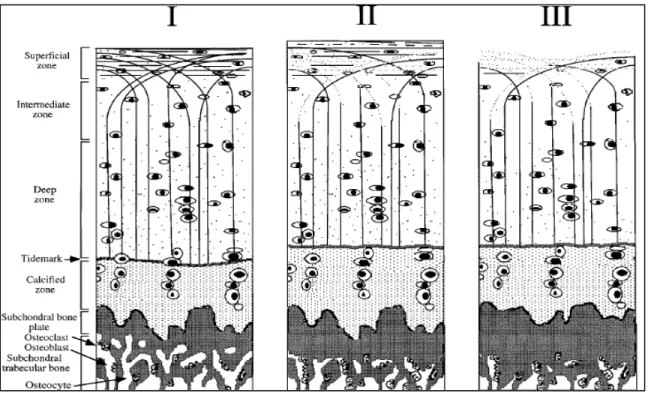
Figure adapted from (Clements et al., 2001) ...10 Figure 1-6 Articular cartilage structure. Chondrocytes (ovals), proteoglycans (dots)
and collagen fibrils (curved lines). The normal histology of the cartilage (left). The onset of OA (middle): Depletion of proteoglycans and
disorganization of collagen fibrils in the superficial zone. Point of no return (right): Fibrillation of the superficial zone, additional loss of
proteoglycans, and subchondral bone sclerosis, adapted from (Arokoski et al., 2000). ...11 Figure 1-7 A hypothetical framework for the initiation and progression of OA. OA
initiation begins with a change in the contact locations of the joint. Cartilage in the less loaded regions Show signs of damage and surface fibrillation under the higher-than-normal loading conditions. Increased friction due to damage to the cartilage causes more severe degeneration of the tissue stimulating the progression of the cartilage breakdown. Figure adapted from (Andriacchi et al., 2004) ...16 Figure 1-8 EOS® low-dose imaging system and the reconstruction of the 3D
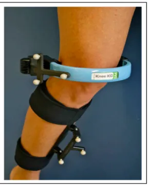
geometry of the bones using a pair of biplane X-ray images. Adopted from http://www.eos-imaging.com, 2016 ...19 Figure 1-9 Reconstruction of the bone using EOS® biplane X-ray images. ...20 Figure 1-10 Anterior view of a right knee fitted with the KneeKG ™ system. Secure
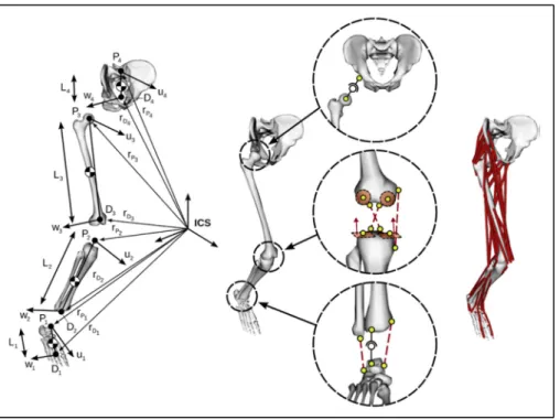
Figure 1-11 Computational framework of the MSK model used to calculate the musculotendon and contact forces. All variables are defined in the
following text. Adapted form (Raphael Dumas et al., 2018) ...25 Figure 1-12 Lower limb parametrization with natural parameters (left). The kinematic
constraints for the hip knee and ankle joints. Figure adapted from (Florent Moissenet et al., 2012) ...26 Figure 3-1 (a) Subjects performed a quasi-static squat assisted by a positioning jig
standardized to put the knee in desired flexion angles. 5 pairs of
orthogonal X-ray images of the lower limb at 0ᵒ, 15ᵒ, 30ᵒ, 45ᵒ, and 70ᵒ of knee flexion were recorded. (b) Bones were reconstructed from bi-planar X-ray images and registered to each of the 5 squat positions the subjects adopt in the EOS® system cabinet. (c) 2 pairs of points on the medial and lateral sides of the tibia and femur represented CPs and minimum tibio-femoral bone-to-bone distances. ...43 Figure 3-2 Origin of femur (Of): midpoint of 2 spheres fitted on the posterior femoral
condyles. Proximal/distal axis of femur (Yf): Of - center of the femoral head. Zc: axis connecting centers of the posterior condyles.
Anterior/posterior axis of femur (Xf): cross product of Yf and Zc, oriented anteriorly. Medial/lateral axis of femur (Zf): cross product Xf × Yf. Origin of tibia (Ot): center of intercondylar eminence. Proximal/distal axis of tibia (Yt): midpoint of the medial and lateral malleoli – Ot. Zp: axis passing through the posterior extremes of the tibial plateaus.
Anterior/posterior axis of tibia (Xt): cross product of Yt and Zp, oriented anteriorly. Medial/lateral axis of tibia (Zt): cross product Xt × Yt
(Südhoff, 2007). ...45 Figure 3-3 Illustrates the average CP trajectories for all the OA and healthy subjects
normalized on a right tibial plateau, and are presented in 5 positions of squat from 0ᵒ-70ᵒ flexion. ...46 Figure 3-4 Average CP trajectories in 10 healthy (blue) and 9 OA (red) subjects
during squat, normalized over a tibial plateau. CP locations are plotted at 0ᵒ, 15ᵒ, 30ᵒ, 45ᵒ and 70ᵒ flexion. Error bars stand for standard deviations (±1 SD). Dashed arrows represent CP movements from 0ᵒ to 30ᵒ or 70ᵒ flexion, in medial/lateral or anterior/posterior direction of healthy (blue) or OA (red) subjects. ...47 Figure 3-5 Quasi-static kinematics of OA and healthy joints during the controlled
squat. Medial/lateral (a) and anterior/posterior (b) displacement of femur with respect to tibia, and internal/external rotation (c) as well as
adduction/abduction (d) of tibia are illustrated as a function of 5 squat positions designed to reproduce 0◦, 15◦, 30◦, 45◦, and 70◦ of flexion
respectively. * denotes a pair-wise significant difference between OA and healthy groups. ...50 Figure 3-6 Tibiofemoral joint imaged from 2 different angles using EOS® biplane
images. The tibial plateau in the left pair of images is viewed from a tight angle where the anterior and posterior edges in the X-rays are
superimposed. The right pair of images is the joint images at a different posture where the edges are not superimposed. ...56 Figure 3-7 Manual multi-view reconstruction/registration using EOS® biplaneX-ray
images ...57 Figure 3-8 Weighted center of proximity algorithm for calculation of contact points.
Higher weights are assigned to the closest regions ...58 Figure 3-9 The minimum bone-to-bone distance is 0.52mm using a coarse mesh
(left), and 0.45mm using a fine mesh. ...58 Figure 3-10 Algorithm of validation of the contact parameters estimated by a
reconstruction/registration process using stand-alone bi-planar X-ray images, versus a set of controlled movements applied to a set of bones reconstructed from a CT-scan. ...60 Figure 3-11 Average medial and lateral CP locations for healthy and OA, on the
medial and lateral plateaus versus BMI ...63 Figure 4-1: Force platform in the EOS® cabinet measures the forces under the studied
foot in the middle while the contralateral foot is isolated from the force platform. ...68 Figure 4-2 Illustration of the placement of the orthosis with respect to the joint. ...74 Figure 5-1 Contact point trajectories of subject N10 from the three contact point
trajectory models over the tibial plateau: linear contact point (LCP) trajectory (: black), sphere-on-plane (SPP) trajectory (-- blue), and personalized contact point (PCP) trajectory (- red) models. The sequence of stance phase events is illustrated on each contact point trajectory: first and second peaks of medial (pk1 Med, pk2 Med), first and second peaks of lateral (pk1 Lat, pk2 Lat) contact force, heel strike (HS), toe off (TO), 0ᵒ (flx0) and 70ᵒ (flx70) knee flexion. The shaded region around the PCP model represents the uncertainty of estimating the weighted center of bone-to-bone proximity (±3 mm) in the medial/lateral direction (Zeighami et al. 2016). ...84 Figure 5-2 Medial, lateral, and total contact forces as well as the knee
Internal/external (Int-Ext) rotations, lateral-medial (Lat-Med),
anterior/posterior (Ant-Post), and proximal/distal (Prox-Dist) translations of subject N10 using the linear contact point (LCP) trajectory (:black), sphere-on-plane (SPP) trajectory (--blue), and personalized contact point (PCP) trajectory (-red) models. The corresponding contact point
trajectories are presented in Figure (5-1). ...86 Figure 5-3 The average (10 subjects) first and second peaks of medial (pk1 Med, pk2
Med) , first and second peaks of lateral (pk1 Lat, pk2 Lat) , first and second peaks of total (pk1 T, pk2 T) contact forces using the linear contact point (LCP) trajectory, sphere-on-plane (SPP) trajectory, and personalized contact point (PCP) trajectory models. * and @ denote statistically
significant differences between the SPP and LCP models and between the SPP and PCP models respectively. ...87 Figure 5-4 First (red marks) and second (blue marks) peaks of the medial and lateral
contact forces (pk1 Med, pk2 Med, pk1 Lat, pk2 Lat) from the
personalized contact point trajectory (PCP) model and the location of the personalized contact points at the corresponding events. Coordinates of the points are presented in Table 1 for all 10 subjects. The dashed line represents the regression line on the medial side (r=0.53, p<0.001). No correlation existed on the lateral side (r=0.18, p=0.43). Results adapted from two previous sensitivity analysis studies are also presented. The range of contact point perturbations were ±25±10 mm in Saliba et al. (2017), and ±20±4 mm in Lerner et al. (2016). ...88 Figure 5-5 Medial, lateral, and total contact forces of the healthy and OA subjects
during the stance phase ...93 Figure 5-6 Placement of reflective markers on the lower limb to track the 3D motion
of the limbs. ...94 Figure 5-7 shows the difference in contact force estimations at the 1st and 2nd medial
and lateral peaks between the personalized contact point (PCP) and linear contact point (LCP) models. The horizontal axis is the personalized medial/lateral contact point location at the corresponding events: pk1 med (first peak of medial force), pk1 lat (first peak of lateral force), pk2 med (second peak of medial force), and pk2 lat (second peak of lateral force). The medial and lateral contact points in the LCP model were always located at -20 mm and +20 mm from the plateau centreline. ...95 Figure 5-8 Difference between the contact force estimated using personalized contact
point and linear contact point models on the vertical axis and the
Figure 6-1 Box and whisker plot of contact forces of the healthy (blue) and OA (red) groups at the 1st and 2nd peaks of medial contact force (pk1 Med, pk2 Med), 1st and 2nd peaks of the lateral contact force (pk1 Lat, pk2 Lat), 1st and 2nd peaks of the total contact force (pk1 T, pk2 T), and the average medial (mean Med) and lateral (mean Lat) contact forces during the stance phase. The plot represents the minimum, maximum, lower and higher quartiles, and the median as well as the mean value (X mark), and the outliers (o mark). ...109 Figure 7-1 Individual contact point trajectories of 9 OA (red) and 10 healthy (blue)
subjects described in chapter 3 ...122 Figure 7-2 MR and ( , ) max( ) (1 ) max( ) KAM f KAM KFM KFM KAM KFM = × + demonstrating similar patterns in one healthy (left), and one OA (right) subject. ...125
LIST OF ABBREVIATIONS
OA Osteoarthritis
ACLD Anterior cruciate ligament deficiency, or deficient ACLR Anterior cruciate ligament reconstructed MCL Medial collateral ligamen
LCL Lateral collateral ligament ACL Anterior cruciate ligament PCL Posterior cruciate ligament ECM Extracellular matrix
K-L Kellgren-Lawrence OA grading system NSAID Nonsteroidal anti-inflammatory drugs MRI Magnetic resonance imaging
CT-scan Computed tomography-scan
RMS Root mean square
SSM Statistical shape model
MSK Musculoskeletal
TKA Total knee arthroplasty
BW Body weight
DOF Degrees of freedom
MR Medial-to-total contact force ratio
KFM Knee flexion moment
KAM Knee adduction moment
Fmed Medial contact force
CPz Medial/lateral contact point location CPx Anterior/posterior contact point location
CPzmed Medial/lateral contact point location on the medial compartment CPzlat Medial/lateral contact point location on the lateral compartment CPxmed Anterior/posterior contact point location on the medial compartment CPxlat Anterior/posterior contact point location on the lateral compartment
FE Finite element
CRCHUM Centre de recherche, centre hospitalier de l’Université de Montréal ÉTS École de technologie supérieure de Montréal
CP Contact point
ANOVA Analysis of variance BMI Body mass index (BMI)
KOOS Knee injury and Osteoarthritis Outcome Score
LCP Linear CP trajectory SPP Sphere-on-plane trajectory PCP Personalized CP trajectory RF Rectus femoris VL Vastus lateralis VM Vastus medialis TA Tibialis anterior GM Gastrocnemius medialis GL Gastrocnemius lateralis ST Semitendinosus BF Biceps femoris
PSA Power spectrum analysis
LIST OF SYMBOLS
3 3×
E Identity matrix
i Index for segment
j Index for skin or virtual marker (in inverse kinematics) or muscle (in inverse dynamics)
ui, vi, wi Anterior, superior and lateral axes of the segment ,
i i
P D
r r Positions of the proximal (Pi) and distal (Di) endpoints
(
)
, , i i , i i i P D i P − v u r r w Non-orthonormal segment coordinate system
(
P X Y Zi, , ,i i i)
Orthonormal segment coordinate systemBi Transformation matrix from the non-orthonormal to the orthonormal segment coordinate system
αi, βi, γi Constant angles between the axes of the non-orthonormal segment coordinate system
Li Segment length (between proximal and distal endpoints)
Qi Natural coordinates (2 position and 2 direction vectors)
r i
Φ Rigid body constraints
, j j i i
M V
r r Position of skin or virtual marker (Mijor j i
V )
( ) ( ) ( )i , , i i
u v w
n n n Coordinates in the non-orthonormal segment coordinate system i
N Interpolation matrix
k
Φ Kinematic constraints
θ Tibiofemoral extension/flexion angle
m
Φ Driving constraints
G Generalised mass matrix
, ,
Q Q Q Vectors of generalized positions, velocities and accelerations for all
segments
λ Vectors of Lagrange multipliers
R Vector of generalized ground reaction forces and moments 2T
K
Z Orthogonal basis of the null space of 2
T
K (corresponding to a subset of
the constraints)
P Vector of generalized weights
L Matrix of generalized muscular lever arms
F Vector of musculo-tendon forces
f, J Objective functions in inverse kinematics and inverse dynamics
INTRODUCTION
Knee osteoarthritis (OA) is a degenerative joint disease characterized by loss or deterioration of articular cartilage. It happens when the cartilage is unable to normally repair itself resulting in the breakdown of the cartilage tissue and the subchondral bone. OA primary clinical manifestations include swelling, pain, stiffness, and decreased range of motion. Known treatments are not effective to stop or slow down OA progression, but they rather address the symptoms of the disease. OA affects more than 10% of Canadian adults and is one of the main causes of chronic musculoskeletal disabilities worldwide. As the population ages, a growing number of OA disability is expected in the future.
There are two types of factors which are known to be responsible for OA initiation and progression: systematic factors such as gender, age, genetics, and racial characteristics and biomechanical factors such as joint overloading, obesity, joint deformity, and joint injury. Systematic factors are believed to establish the foundation of cartilage properties whereas the biomechanical factors determine the location and severity of cartilage degeneration (Arokoski 2003). Biomechanical abnormalities can be detrimental to the tissue by exposing the cartilage to excessive contact forces or by changing the contact point locations from the frequently loaded regions to the regions that are not usually loaded. Subtle kinematic abnormalities triggered by conditions such as anterior cruciate ligament deficiency (ACLD), shift the contact point locations from the frequently loaded regions and causes cartilage thinning which is an early sign of OA initiation (S Koo et al., 2007).
High levels of contact forces could also damage the cartilage. While some level of repetitive loading is required for the nutrient distribution through the cartilage and regeneration of the tissue structure, excessive contact forces could damage cartilage by killing the cartilage living cells (chondrocytes), which regenerate and maintain the tissue structure (Clements et al., 2001). In the knee joint, the medial compartment carries a bigger proportion of the contact forces and is more likely to be affected by OA than the lateral compartment. The larger forces on the medial compartment are due to the line of ground reaction force which falls medial to
the knee joint center creating an external adduction moment in the frontal plane. However, studies have argued that other parameters such as knee flexion moment, knee frontal plane alignment, gait speed have also a significant contribution to the contact force distribution (Adouni et al., 2014; Esculier et al., 2017; Kumar et al., 2013; Kutzner et al., 2013). In addition, since the external knee moments are counterbalanced partially by the medial and lateral contact forces, the contact point locations would also contribute to the contact force distribution (Lerner et al., 2015; Saliba et al., 2017b).
According to what was discussed above, the knee contact point locations and contact forces are the two main biomechanical parameters in understanding the pathomechanics of OA. Thus, it is crucial to understand the patterns of contact points and contact forces and also, the relationship between these two parameters in OA and healthy subjects. This latter requires knowledge of the personalized contact points and the inclusion of these personalized contact points in the contact force estimations. Until now, the literature has not provided a quantitative description of the contact points in OA subjects in comparison with healthy controls. Moreover, the attempts to personalize the knee kinematic models in OA subjects does not address directly the contact points (Clément et al., 2017; Lerner et al., 2015). None of knee kinematic models introduced in musculoskeletal model currently allow evaluating the impact of the pathology distinct patterns of contact points on the contact force estimations.
The general objective of this thesis is to evaluate the tibiofemoral contact locations and the contact forces in OA subjects and to analyze the differences with respect to the healthy subjects. Chapter 1 provides an introduction on the function and anatomy of the knee joint, the mechanisms of OA and discusses the current body of the literature on the tibiofemoral contact points and contact forces in normal and pathological knees and the methodological aspects of estimating these parameters and their limitations. Chapter 2 lists the problematics, aims and specific objectives of the current work. Chapter 3 introduce a method to estimate the personalized contact points during a weight-bearing squat activity from a set of biplane X-ray images and a 3D/2D registration techniques. The contact point locations in OA and healthy subjects are compared to examine the existence of a shift in the contact point locations of OA
joints with respect to the healthy ones. Chapter 4 provides the preliminary results on evaluating the effectiveness of a valgus knee orthosis in changing the contact point locations of severe OA subjects during squat. This gives a clinical example of the use of contact point locations as a novel metric for assessing the effectiveness of the interventions planned to improve the ambulatory function of subjects with OA. Chapter 5 introduces a method for the integration of the personalized contact points in the musculoskeletal model of the lower limb when estimating the contact force. Chapter 6 uses the musculoskeletal model with the personalized contact points to compare the medial and lateral contact forces in OA and healthy subjects. We also evaluated the contribution of contact point trajectories in the medial-to-total contact force ratio in the knee joint and determined the parameters with the highest contribution in OA and healthy subjects. Chapter 7 presents a general discussion summarizing the results of the four studies and remind the various limitations of the project and makes recommendations for the further projects. Finally, a general conclusion with the principal contributions ends this thesis.
CHAPTER 1 LITERATURE REVIEW 1.1 Structure and anatomy of the knee joint
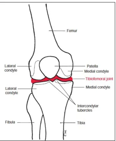
The knee represents one of the most voluminous joints and surely one of the most complex of the human body. It is composed of two main joints, one being the junction between the two main long bones of the lower limb, i.e. the femur and the tibia (tibiofemoral joint), and the second between the femur and the patella (patellofemoral joint) (Figure 1-1). Although these two articulations are anatomically and functionally related, this project will focus on the tibiofemoral articulation.
1.1.1 Structure and components of the tibiofemoral joint
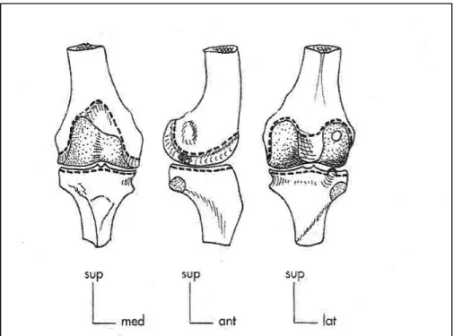
The tibiofemoral joint is a double load carrying joint. The articulation (Figure 1-2) is composed of the femoral and tibial condyles which are located at the medial distal and lateral distal ends of the femur and at the proximal medial and proximal lateral ends of the tibia respectively. The convex shape of the femoral condyles articulates with the slightly concave surface of the tibial condyles granting significant mobility to the knee in the six degrees of freedom. The articulating surfaces are covered by a thin layer of articular cartilage allowing an efficient lubrication. The low congruence of the joint surfaces leaves limited contact surface that may be the cause of high contact pressures. This is, however, attenuated by the presence of two menisci attached to the peripheral edges of the tibial condyles. The crescent-shaped menisci with fibrocartilaginous structure, make it possible to distribute articular pressures over a larger contact area. The medial meniscus is narrow and long in shape of a "c" while the lateral meniscus is wider as well as shorter in the shape of an "0" (Figure 1-3). The menisci are slightly deformable structures during movement, but they remain firmly anchored at the joint surfaces by the meniscal attachments.
A set of ligaments provide stability to the tibiofemoral joint. Medial collateral ligament (MCL), Lateral collateral ligament (LCL), Anterior cruciate ligament (ACL), and Posterior cruciate ligament (PCL) are the four main knee joint ligaments.
Collateral ligaments are necessary to prevent rotation in the frontal plane around the anteroposterior axis when the knee is in extension, while cruciate ligaments help to prevent anteroposterior translation of the articular surfaces by connecting the tibia and femur.
Meniscus and ligament pathology are in some cases primary to OA. A long-term change in the dynamics of knee loading due to ligament or meniscus injury is associated with a very high risk of OA development (Lohmander et al., 2007).
Figure 1-1 Anatomy of the knee and the tibiofemoral joint. Figure adapted from Norkin et al. (2016).
Figure 1-2 Tibiofemoral articulation viewed from anterior (left) lateral (middle) and posterior (right) directions, allowing to illustrate the shape of the femoral and tibial condyles, adapted
from Dufour (2007).
Figure 1-3 Top view of the tibial plateau showing the shape of the medial (1) and lateral (2) menisci and their corresponding attachments (3,4). The figure is adapted from (Dufour,
1.1.2 Structure and composition of articular cartilage
Knee articular cartilage is a thin layer of hyaline cartilage specialized to provide a smooth and efficient lubrication between the joint surfaces. This tissue has no nerves, blood vessels, or lymphatics. It rather consists of an extracellular matrix (ECM) structure in which a type of cells called chondrocytes is scarcely distributed. The ECM structure is principally formed from collagen and proteoglycans and retains a substantial amount of water (Sophia Fox et al., 2009). This water is gently released under pressure and provides cartilage its unique lubrication properties under dynamic loading. The components of the cartilage are briefly described in the following.
1.1.2.1 Water
Water accounts for about 65 % - 80% of the wet weight of articular cartilage in deep and superficial zones respectively (Baykan, 2009). Water has two main roles in the cartilage being the distribution of nutrients and giving special mechanical properties to the cartilage. Unlike other organs and tissues, cartilage is devoid of nutrient carrying blood vessels. The nutrients to chondrocyte cells are transported through the flow of fluid in and out of the cartilage. Articular cartilage has the ability to withstand significant loads while maintaining minimal friction thanks to the interstitial fluid in its structure. Under loading, the fluid inside the cartilage which cannot escape easily from the surface is pressurized and transfers a major proportion of the load. Meanwhile, the water flow minimizes the solid-to-solid friction and makes the cartilage very efficient in lubrication.
1.1.2.2 Collagens
Type II collagen molecules represent ~75% of the dry weight of the cartilage. Collagen molecules form small fibrils and larger fibers distributed throughout the cartilage with depth-dependent dimension and orientation. The specific architecture of the collagen fibrils
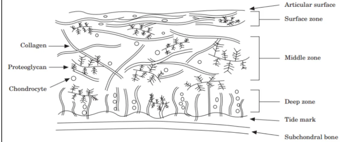
contributes to the stability of the ECM and provides cartilage with important shear and tensile properties. In the superficial zone, collagen fibrils are packed tightly and aligned parallel to the surface to better resist shear and tensile forces imposed by articulation. They are oriented obliquely in middle zone and perpendicularly in the deep zone to provide the highest resistance to the compressive forces (Figure 1-4).
Figure 1-4 Scheme of articular cartilage structure, adapted from Fox et al. (2009)
1.2 Cartilage loading and OA progression
Progression of OA occurs during a long period of time. However, due to the lack of nerves in the cartilage tissue the symptoms appear towards the end stages. At this point, OA cannot be stopped or reversed. Therefore, it is crucial to understand the initiation and progression mechanisms. These mechanisms are largely unknown. But, it is generally thought that the initiation and progression of OA are associated to the mechanical properties and structure of cartilage on one hand and the joint loading on the other hand (Herzog et al., 2006).
1.2.1 Mechanical loading effect on cartilage
Mechanical loading has a double effect on the cartilage tissue. Given the nature of nutrient distribution with the fluid flow throughout the cartilage, loading has a great impact on the
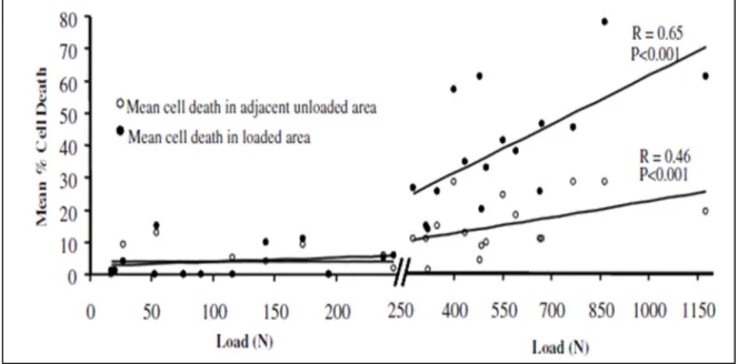
synthesis of proteoglycan molecules. Normal cyclic loading of the cartilage promotes proteoglycan synthesis and makes it stiffer. It is reported that a cartilage regularly exposed to some levels of stress contains a higher amount of proteoglycans (Arokoski et al., 2000). On the other hand, continuous high-stress levels in the cartilage diminish proteoglycan synthesis and result in damages to the tissue through necrosis. Clements et al. (2001) suggested a threshold over which the chondrocytes would dye under cyclic loading. In a bovine cartilage experiment, they reported this threshold to be 6 Mpa. Over this threshold, the chondrocyte viability was negatively correlated to the magnitude of applied stress (Figure 1-5).
Figure 1-5 cyclic loading over 6 Mpa kills the chondrocytes in bovine cartilage. Figure adapted from (Clements et al., 2001)
Decreased proteoglycan concentration, disorganization of the collagen network, and softening of cartilage are the early signs of OA and cartilage injury (Figure 1-6). It is believed that once the integrity of the superficial zone of cartilage is lost, the underlying tissue would experience abnormally high strains. Thereafter, the degenerations would extend into the deeper zones of cartilage (Figure 1-6) (Arokoski et al., 2000). In the initial stage, the cartilage loses volume and becomes more vulnerable to damage under excessive load. The subchondral bone thickens
and fluid-filled cysts may appear near the joint. Eventually, broken bone or cartilage particles may float in the joint triggering further mechanical damage.
Figure 1-6 Articular cartilage structure. Chondrocytes (ovals), proteoglycans (dots) and collagen fibrils (curved lines). The normal histology of the cartilage (left). The onset of OA (middle): Depletion of proteoglycans and disorganization of collagen fibrils in the superficial
zone. Point of no return (right): Fibrillation of the superficial zone, additional loss of proteoglycans, and subchondral bone sclerosis, adapted from (Arokoski et al., 2000).
1.2.2 Mechanical behavior of cartilage as an indicator of OA
Following the histopathological and structural changes of cartilage due to OA progression, its mechanical characteristics change as well. Softening of cartilage in the initial stage is reported in some papers. In a study on different parts of cartilage collected during total knee arthroplasty, Kleemann et al. (Kleemann et al., 2005) found a meaningful correlation between OA severity and the reduction in the cartilage stiffness.
Other studies showed that in artificially made OA through ACL transaction shear, tensile, compressive and other mechanical behaviors of cartilage are considerably changed (Setton et
al., 1999). It indicates that the mechanical, structural, and histological changes of cartilage during OA are interrelated. The results indicated a relation between structural, mechanical and histological changes in all stages of the degeneration. With increasing grade, the cartilage stiffness, which is primarily influenced by the integrity of the extracellular matrix, decreases and so are other mechanical properties.
1.3 OA demonstrations and grading of the disease
Regarding the histopathological changes in cartilage different scoring and grading methods are presented to classify the development of disease (Collins, 1939; Mainil-Varlet et al., 2003; Mankin et al., 1971). A histopathological grade assessment guide is presented in Table 1-2 based on Pritzker’s method (Pritzker et al., 2005) to indicate what generally represents the step by step OA progression in different stages.
The mainstay tool for diagnosis and monitoring of OA is plain radiography. Therefore, the classification of the disease is commonly performed using the manifestations observed in radiographic images. Kellgren-Lawrence (K-L) is among the most popular OA classification tools which describe the severity of OA based on a 0 to 4 grading system (Kellgren et al., 1957; Schiphof et al., 2008). The K-L grading system was used in this thesis to discriminate the severe OA subjects and healthy controls.
Table 1-1 Kellgren-Lawrence OA grading system and each grade characteristics. Adapted from Kohn et al. (2016).
Kellgren-Lawrence scale grades Characteristics
Grade 0 No Joint space narrowing or reactive changes
Grade 1 Doubtful joint space narrowing, possible osteophytic lipping Grade 2 Possible joint space narrowing, definite osteophytes.
Grade 3 Definite joint space narrowing, moderate osteophytes, some sclerosis, possible bone-end deformity
Grade 4 Marked joint space narrowing, large osteophytes, severe sclerosis, definite bone ends deformity
Table 1-2 Pritzker’s histopathological grade assessment guide indicating the
histopathological changes of cartilage during OA progression. Adapted from (Pritzker et al., 2005).
1.4 Altered gait and anatomy characteristics in patients with OA
The gait differences in OA subjects has been the subject of previous studies. Symptomatic OA subjects experience pain performing daily activities. This may result in adopting compensating gait strategies to reduce joint loading and the resultant pain (Stauffer et al., 1977). Reduced range of knee flexion is a remarkable pattern in the gait of OA patients (Schnitzer et al., 1993; Stauffer et al., 1977). Kaufman et al. (2001) reported 6° reduced range of motion and significantly lower gait speed in OA patients. The stride characteristics were also altered in OA group. Stride length was significantly smaller in OA subjects whereas cadence increased with respect to healthy controls (Kaufman et al., 2001). Knee varus alignment is another typical feature in OA and is believed to make the joint more vulnerable to the adverse effects of obesity and joint overloading (Sharma et al., 2000).
External moments, and in particular adduction moment has been found to be associated with OA in many studies. Baliunas et al. (2000) observed increased peak of adduction moment in OA subjects. Adduction moment has been found to correlate with severity (Schnitzer et al., 1993) or progression (Miyazaki et al., 2002) of OA. Adduction moment was also found to be correlated with the bone density of the proximal tibia (Hurwitz et al., 2002) and the outcome of tibial osteotomy surgery (C. Prodromos et al., 1985; Wang et al., 1990). Knee flexion moments is also one of the altered characteristics of gait in OA subjects. The peak of knee flexion moment decreased in OA subjects with respect to healthy controls (Baliunas et al., 2000; Kaufman et al., 2001).
The mechanism behind the biomechanical alterations in OA is not fully understood. It is known that mitigating knee joint pain in some subjects can reverse some of these changes. For instance, following 4 weeks of treatment with nonsteroidal anti-inflammatory drugs (NSAID), the maximum adduction moment and quadriceps moment (measured on ergometer) increased due to the joint pain reduction (Schnitzer et al., 1993). However, some biomechanical alterations are attributed to the morphological changes such as joint space narrowing in OA knees which permanently change the configuration of the joint and, as a result, the dynamics of the joint. Relieving the pain, in this case, would not make a difference. In a study on medial
compartment OA subjects and healthy controls, Andriacchi et al. (2004) reported that the varus alignment and the adduction moment were similar between healthy and moderate OA subjects whereas they were significantly different in severe OA patients who had a remarkable joint space narrowing in the medial compartment. Andriacchi et al. (2004) hypothesized that the change in the varus alignment and the adduction moment are a result of the change in the morphology of the joint in severe OA.
1.5 Altered tibiofemoral contact point in patients with OA
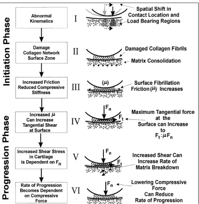
Along with the morphological changes of the joint, the tibiofemoral joint surface interpositions change as well. It is assumed that the initiation of OA begins with a change in the contact locations of the joint to the regions where it is not frequently loaded (Andriacchi et al., 2004). This shift could follow a traumatic or chronic condition such as meniscus or ligament injury. Loading the regions that are not conditioned to carry high frequent loads is detrimental to the cartilage tissue resulting in fibrillation of the surface and further damage to the tissue. Surface fibrillation causes an increase in the surface friction which induces further damage to the cartilage and accelerates the progression of the disease (Figure 1-7). However, the experimental data supporting this hypothesis on the pathomechanics of the knee OA is scarce.
Figure 1-7 A hypothetical framework for the initiation and progression of OA. OA initiation begins with a change in the contact locations of the joint. Cartilage in the less loaded regions
Show signs of damage and surface fibrillation under the higher-than-normal loading conditions. Increased friction due to damage to the cartilage causes more severe degeneration
of the tissue stimulating the progression of the cartilage breakdown. Figure adapted from (Andriacchi et al., 2004)
Using dual fluoroscopy, Farrokhi et al. (2014) found that in OA subjects with self-reported instability the excursion and velocity of the medial compartment contact points were
significantly increased with respect to the healthy controls. In a later study, they showed that the increased velocity and excursion of contact points in OA group was associated with the increased frontal plane alignment. Increased contact point (CP) excursion in OA was therefore considered as a measure of mechanical instability of the affected joint (Farrokhi et al., 2016). In this regard, in the biomechanical analysis of the knee joint in OA, it is important to consider the configuration of the joint and the interaction of the articulating bones along with the other parameters of gait. This will help to better understand the parameters contributing to the pathomechanics of OA.
1.6 Tibiofemoral contact point estimation
Estimating the in vivo tibiofemoral contact points provides precious information that is valuable in understanding the initiation and progression mechanism of OA. It is hypothesized that the initiation of cartilage degeneration is triggered by a shift in the tibiofemoral contact point locations from the frequently loaded parts of the joint close to the tibial plateau centerlines towards the less loaded regions (T. P. Andriacchi, 2004). Positioning the contact point is also important in designing total knee arthroplasties and developing the customized or personalized musculoskeletal models (Lerner ZF, 2015 Feb 26).
Identification of joint contact parameters utilizing casting and pressure sensitive films are only practical in cadaver models (Ahmed et al., 1983; Walker et al., 1985). Magnetic resonance techniques normally scan the knee joint statically in supine posture and have technical limitations in studying naturally loaded joints and large ranges of motion (Johal et al., 2005; Yao et al., 2008). Therefore, 3D/2D registration techniques have been widely used to track the in vivo 3D motion of the bones in load-bearing conditions. The bone is generally reconstructed from magnetic resonance imaging (MRI) or computed tomography (CT)-scan with or without the cartilage layer, and then rigidly moved to match the 2D fluoroscopic or X-ray images recorded during movements. Tibiofemoral contact points are then estimated using the proximity of the articulating surfaces.
1.6.1 Reconstruction of subject-specific bone using imaging techniques
The geometry of the knee joint for analysis of the joint is usually reconstructed from a stack of images obtained from MRI or CT-scan of the joint. The MRI is typically preferred for the soft tissues reconstruction, whereas CT images are widely used for hard tissues i.e., bones (Kazemi et al., 2013). MRI does not emit ionizing radiation that makes it minimally detrimental to the patient. Both imaging methods provide segmentation accuracy with a root mean square (RMS) error below twice the pixel size. For a 1.5T MRI, this accuracy is less than 1mm. However, MRI is relatively costly, time-consuming in each acquisition and is normally performed only in supine position. CT-scan, on the other hand, exposes the subject to high levels of ionizing radiations making it potentially detrimental particularly in larger scale reconstructions such as the whole lower body.
1.6.2 Reconstruction of subject-specific bone using X-ray images
The radiographic images are the most clinically available data in assessing OA subjects and they show hard tissue boundaries with a very good resolution. The ability to reconstruct the 3D patient-specific surface model of a bone from a limited number of 2D X-ray images (2 or more) would be clinically valuable. Various manual, semi-automatic and automatic solutions were proposed for this purpose. One solution is using a statistical shape model of the bone and adapting it to the personalized biplane X-ray of the subject to approximate the individual 3D geometry (G. Zheng et al., 2009).
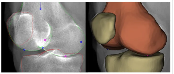
Another solution was proposed using EOS® system (EOS imaging, Paris, France) biplane X-ray images and a generic model of the bone. The EOS® system simultaneously captures 2 perpendicular images of the whole (or lower) body of standing subject in a single scan with a 1:1 vertical scaling. Generating the geometric models of the bone structures of the knee with the EOS® system requires segmenting the bone contour in the biplane radiographs (Chav et al., 2009). Then, a generic bone model is deformed semi-automatically until it is superimposed
on the contours segmented in the previous step (Thierry Cresson et al., 2010; Cresson et al., 2008) (Figure 1-9).
Figure 1-8 EOS® low-dose imaging system and the reconstruction of the 3D geometry of the bones using a pair of biplane X-ray images. Adopted from http://www.eos-imaging.com,
2016
A major advantage of the EOS® system is its low emission of ionizing radiation; at the level of the spine, it has been estimated 8 to 10 times less than that of conventional radiography, and 800 to 1000 times less than CT-scan (Deschênes et al., 2010; Dubousset et al., 2005). The main drawback of this procedure is that segmentation of soft tissue and cartilage is not possible. Only hard tissues are well visualized in X-ray images.
Figure 1-9 Reconstruction of the bone using EOS® biplane X-ray images.
1.6.3 3D kinematics tracking of bones using biplane images
The techniques to study in vivo 3D knee kinematic include a 3D reconstruction of the geometry using CT-scan, MRI, or biplane radiographs (EOS®) and then matching the model to the 2D projections of the joint captured during joint movement. Tashman et al. (2003) used a combination of CT and high-speed biplane radiography to measure the joint motion. (G Li et al., 2001) performed a computational analysis on the cartilage with the cartilage contact calculated using a reconstruction of bone and cartilage from MRI and movement tracking by 2D fluoroscopic images.
In the current project, we use the 2D images captured in EOS® in a standing position to reconstruct the shape of the bone. For the kinematics tracking, the 3D reconstructed geometry is matched to the biplane EOS® images of the subject taken at different flexion angles. The reconstruction/registration procedure is performed in IdefX software through the steps as described in (Chaibi et al., 2010). Further technical details are provided in chapter 3.
Previous studies have been conducted on kinematics tracking using EOS® images. In a cadaveric study, Azmy et al. (2010) combined EOS® 3D reconstructions with an
optoelectronic motion capture system for measuring tibiofemoral and patellofemoral pseudo-kinematics. They reported the overall rotational and translational uncertainty below 0.4° and 1.8 mm for the tibiofemoral and 0.4° and 1.2 mm for the patellofemoral kinematics respectively.
Other studies used stand-alone EOS® X-ray images for both geometry reconstruction and motion registration processes to study squat task (Clément et al., 2015, 2017). Some studies developed automated techniques for the 3D/2D registration step while others used manual registration. Südhoff et al. (2007) used EOS® reconstruction/registration as a reference to compare three attachment systems and harnesses designed to measure the 3D kinematics of the knee. All three were installed on subjects during pseudo-dynamic squats in the EOS® system. Thus, the tibiofemoral kinematics measured by the attachment systems and harnesses could be compared to that from EOS® system as a reference. Jerbi et al. (2011) employed an automated registration process based on the frequency domain to track the motion of the bone in healthy and prosthetic subjects. In this case, the manual registration was considered as the gold standard and the registration error was reported 1.5 mm and 1.5° for the healthy group and 0.5 mm 0.8° for the prosthetic group. Michèle Kanhonou (2017) used an iterative closest point algorithm for the 2D/3D registration process and reported the reproducibility of the method 0.4 mm and 0.5°. They also checked the sensitivity of the method to the 3D reconstruction and found the translational and rotational sensitivities to be 1.7 mm and 1.4° respectively.
1.7 Gait Analysis
1.7.1 3D kinematics: Marker tracking using KneeKG™ system
In 3D kinematic studies by marker tracking, reflective or light-emitting markers are attached to the skin surface of the segments whose movements are to be tracked. Their movements are recorded by cameras during a dynamic activity and the 3D kinematics is deduced by processing these data. However, the measured kinematics suffers from measurement inaccuracy induced due to soft tissue artefact, i.e. the sliding of the soft tissues between the markers and the bones.
This soft tissue artefact has been quantified by several teams. By comparing the kinematics calculated using skin markers with respect to the actual movement of the bones measured with fluoroscopy. The errors could reach up to 12 ° and 20 mm for the 3D rotations and displacements respectively (Ganjikia et al., 2000; Sati et al., 1996; Tsai et al., 2015). Others compared the 3D kinematics obtained using skin markers with that calculated using bone embedded implants during walking. Here, maximum mean differences of about 4 ° and between 10.5 mm and 13.7 mm have been reported for the angular and linear displacements (Michael S Andersen et al., 2010; Benoit et al., 2006).
To reduce measurement errors associated with soft tissue artefact, the exoskeleton attachment systems were developed to measure the 3D kinematics of the knee. They exploit the fact that some areas of the lower limb are less prone to movement than others. In the current project, we used the KneeKG ™ system (Emovi inc., Laval, Quebec, Canada) which is an exoskeleton system developed with the objective of providing a reliable analysis of the lower limb kinematics while minimizing the soft tissue artefact (Figure 1-10). The femoral arch of the exoskeleton is installed between the tendons of the biceps femoris and iliotibial band on the lateral side. On the medial side, it is placed between vastus medialis and sartorius tendon. For the tibial portion, the rigid portion of the exoskeleton is attached along the anterior tibia.