Crust-mantle boundary in eastern North America, from the (oldest) craton to the (youngest) rift.

Crust-mantle boundary in eastern North America, from the (oldest) craton to the 1

(youngest) rift. 2

3

Vadim Levin1, Andrea Servali1, Jill VanTongeren1, William Menke2, Fiona Darbyshire3 4

5

1. Department of Earth and Planetary Sciences, Rutgers University 6

610 Taylor Road, Piscataway, NJ, 08854-8066 USA 7

2. Department of Earth and Environmental Sciences, Columbia University 8

P.O. Box 1000, 61 Route 9W, Palisades, NY 10964-1000 USA

9

3. Geotop, Université du Québec à Montréal, C.P. 8888, Succ. Centre-Ville 10 Montréal, Qc, H3C 3P8 11 12 ABSTRACT 13

The North American continent consists of a set of Archean cratons, Proterozoic orogenic 14

belts and a sequence of Phanerozoic accreted terranes. We present an ~1250 km long 15

seismological profile that crosses the Superior craton, Grenville province, and 16

Appalachian domains, with the goal of documenting the thickness, internal properties and 17

the nature of the lower boundary of the North American crust using uniform procedures 18

for data selection, preparation and analysis to ensure compatibility of the constraints we 19

derive. 20

21

Crustal properties show systematic differences between the three major tectonic domains. 22

The Archean Superior Province is characterized by thin crust, sharp Moho and low values 23

of Vp/Vs ratio. The Proterozoic Grenville Province has some crustal thickness variation, 24

near-uniform values of Vp/Vs, and consistently small values of Moho width. Of the three 25

tectonic domains in the region the Grenville Province has the thickest crust. Vp/Vs ratios 26

are systematically higher than in the Superior Province. Within the Paleozoic 27

Appalachian Orogen all parameters (crustal thickness, Moho width, Vp/Vs ratio) vary 28

broadly over distances of 100 km or less, both across the strike and along it. Internal 29

tectonic boundaries of the Appalachians do not appear to have clear signatures in crustal 30

properties. 31

32

Of the three major tectonic boundaries crossed by our transect, two have clear 33

manifestations in the crustal structure. The Grenville Front is associated with a change in 34

crustal thickness and crustal composition (as reflected in Vp/Vs ratios). The Norumbega 35

Fault Zone is at the apex of the regional thinning of the Appalachian crust. The 36

Appalachian Front is not associated with a major change in crustal properties, rather it 37

coincides with a zone of complex structure resulting from prior tectonic episodes, and 38

thus presents a clear example of tectonic inheritance over successive Wilson Cycles. 39

40

1. INTRODUCTION 41

42

The overall chemistry and structure of the Earth’s continental crust requires a complex, 43

multistage process of formation (Rudnick and Gao, 2003). How that process operated 44

over the course of Earth’s history is still a matter of debate. Properties of the continental 45

crust such as its vertical extent, the nature of its boundary with the underlying mantle, 46

and the lateral variability in those parameters, are essential for informing the debate. In 47

order to place better constraints on the formation, evolution, and growth of the 48

continental crust, we have constructed a profile of seismological properties across eastern 49

North America, stretching ~1250 km, from James Bay in central Quebec to the Fundy 50

basin in New Brunswick (Figure 1). 51

52

The North American continent provides an ideal setting to probe Earth’s crustal structure 53

and composition in the context of nearly 3 Ga of geological history. The Superior 54

Province of North America has not experienced major internal deformation for nearly 2.6 55

Ga, preserving crust that was last modified during the Archean. The oldest of the post-56

Archean terranes is the Grenville Province, formed at ~1 Ga and associated with the 57

closure of an ocean basin and supercontinent assembly (Moore, 1986; Whitmeyer and 58

Karlstrom, 2007; Hynes & Rivers, 2010). The Grenville Province contains accreted 59

sections as well as reworked material from the Superior Craton and from 60

Paleoproterozoic-age orogens. The Grenville Province separates the cratonic core of the 61

continent from the younger (0.3−0.4 Ga) Appalachian terranes, which were accreted 62

during the closure of the Iapetus ocean in the Paleozoic (Taylor, 1989; Hibbard et al, 63

2007). Our study crosses the Superior, Grenville and Appalachian domains. Its 64

northwestern end is close to the area of the thickest lithosphere in North America (and 65

globally, e.g. Artemieva, 2006) and some of the oldest rocks (3.8 Ga; David et al., 2009). 66

The southeastern end of our transect is within the Fundy Basin formed during the opening 67

of the Atlantic in the middle-late Triassic (Withjack et al., 1995). 68

69

The seismological profile presented here combines the lateral coverage of continent-scale 70

studies with spatial resolution on the order of 10s of km. Uniform procedures used in data 71

selection, preparation and analysis ensure compatibility of the constraints we derive for 72

the thickness, internal properties and the nature of the lower boundary of the North 73

American crust. Our primary objectives are to explore whether first-order properties of 74

the continental crust have systematic differences for areas with significantly different age 75

of consolidation (e.g., Thompson et al., 2010; Yuan, 2015), and to investigate the way 76

tectonic boundaries seen at the surface extend to depth. The latter goal is facilitated by 77

the denser spatial sampling of regions in the vicinity of the Grenville Front, the 78

Appalachian Front, and the Norumbega Fault Zone, discussed in more detail below. 79

80 81

2. GEOLOGIC SETTING AND TECTONIC HISTORY 82

83

2.1 Tectonic units 84

85

2.1.1 The Superior Craton 86

The Superior craton is the largest of the Archean cratons (Card, 1990). It is made 87

up of several distinct terranes with origin dates as early as 3.8 Ga (David et al., 2009). 88

The northern and southern portions of the Superior craton are dominated by high grade 89

gneisses, whereas the center of the craton is characterized by granite-greenstone and 90

metasedimentary belts (Card, 1990). It is widely considered that the assembly of the 91

Superior craton from these distinctive cratonic blocks occurred mainly during 2.72 Ga 92

and 2.68 Ga collisional events (Percival et al., 2007), though debate exists over the exact 93

style and timing of these events. Amalgamation of the craton occurred by north-south 94

compression and dextral transpression (Card, 1990) with younger terranes more common 95

in the southernmost portions. The transect presented here constrains seismic properties 96

of the La Grande terrane, the Opinaca subprovince, and the Abitibi granite-greenstone 97

belt. In his comprehensive review of Superior craton geology, Card (1990) suggests that 98

the final accretion of the craton occurred by “subduction-driven oblique accretion of 99

oceanic and continental volcanic arcs, accretionary sedimentary wedges, older 100

microcontinental fragments, etc. in a convergent margin setting”. Such a scenario is 101

similar to that proposed for the accretion of the Appalachians to the Laurentian margin 102

approximately 2 billion years later (see below). 103

104

2.1.2 The Grenville Province 105

The Grenville Province exposes a region of intense tectonism associated with the 106

assembly of the supercontinent Rodinia between 1.1 and 0.9 Ga. Surface exposures 107

indicate peak metamorphism of metaigneous and metasedimentary units in the upper 108

amphibolite to granulite facies (6 – 8 kbar; Annovitz and Essene, 1990). Assembly of 109

Rodinia in this region began with accretion of island arc terranes during the Elseviran and 110

Shawiningan Orogenies, followed by continent-continent collision during the later 111

Grenville Orogeny (e.g., Rivers, 2015). 112

113

2.1.3 The Appalachians 114

During the lead up to the assembly of the supercontinent Pangea in the early 115

Paleozoic, four distinct island arc terranes and continental fragments were accreted to the 116

Laurentian margin in eastern North America (van Staal et al., 2009). These accretionary 117

episodes (the Taconic, Salinic, Acadian, and Neoacadian orogenies) are now what define 118

the present day Appalachians. In contrast to that observed throughout the Grenville 119

Province, the majority of surface exposures in the Appalachians correspond to shallow 120

crustal levels (e.g. limestones, shales, upper island arc crust) and are not deeply eroded 121

remnants. Our transect crosses all but one of the classic northern Appalachian terranes: 122

Humber, Dunnage, Gander and Avalon (Hibbard et al., 2007; van Staal et al., 2009). 123

124

2.1.4 Rifting of eastern North America 125

In the region covered by our study, in the Central Segment of the eastern North 126

American rift system, the breakup of Pangea and opening of the Atlantic Ocean took 127

place during the middle Jurassic to late Triassic. Rifting proceeded by a series of 128

asymmetric half-grabens and basement-involved border faults (Withjack et al., 2012). 129

The strike of border faults throughout the eastern North American rift system suggests 130

that faulting was accommodated along previous suture zones associated with the prior 131

orogenesis (Withjack et al., 2012). 132

133

2.2 Major tectonic boundaries 134

135

2.2.1 The Grenville Front 136

The continent-scale Grenville Front (GF) separates the exposure of the Archean Superior 137

province from the Grenville Orogen (Irving et al., 1972; Moore, 1986). Initially believed 138

to be the locus of the continent-continent collision, and thus a quintessential “continental 139

suture” (Dewey and Burke, 1973), the GF has been later interpreted as a major 140

contractional fault system (e.g., Rivers et al., 1989) acting on the former passive margin 141

of the Archean-age continent. In some places the GF accommodates 10 km or more of 142

vertical displacement resulting from northwest thrusting of Grenville Orogen rocks over 143

the foreland to their present-day position (Rivers et al., 1989). Since the end of 144

Mezoproterozoic (~1 Ga, Hynes and Rivers, 2010) there has been little tectonic activity 145

on the GF. Seismic studies (e.g. Green et al., 1988; Martignole et al., 2000; White et al., 146

2000) showed the GF to extend through the middle crust, and in many reconstructions 147

(Rivers et al., 1989; Ludden and Hynes, 2000; Hynes and Rivers, 2010) it is shown to cut 148

the crust and sole into the Moho. Associations of the GF with systematic changes in 149

seismic properties of the lithospheric upper mantle have been proposed by Aktas and 150

Eaton (2006), Frederiksen et al. (2006), and Zhang and Frederikson (2013). 151

152

2.2.2 The Appalachian Front 153

The Appalachian Front (AF), a boundary between the Appalachians and the Grenville 154

Province, follows the St. Lawrence river northeast of Quebec City (e.g., Tremblay et al., 155

2013). Historically referred to as Logan’s Line (Alcock, 1945; Thomas, 2006), it is a 156

clear case of tectonic inheritance (Thomas, 2006), as two episodes of rifting (one 157

successful and one not), and a contractional tectonic front all took place broadly along 158

this boundary. A locus of faulting associated with the opening of the Iapetus ocean in 159

earliest Paleozoic time (Kumarapeli, 1985), and subsequently a northwestern-most reach 160

of the Taconic nappes, the Appalachian Front (AF) is a good example of the mismatch 161

between surface geology and deep crustal lithology as Grenville-age rocks are known to 162

extend east of the AF (Hynes and Rivers, 2010). 163

164

2.2.3 Other boundaries 165

In addition to boundaries demarcating distinct terranes within it, the Appalachian Orogen 166

hosts a number of more enigmatic structures with complex history. The Mesozoic-age St. 167

Lawrence rift is nearly coincident with the AF. The St. Lawrence rift is a site of failed 168

continental separation, and one of the most seismically active areas of Eastern North 169

America (e.g. Lamontagne et al., 2003). Most of the seismicity is localized within a ~350 170

Ma old impact structure (the Charlevoix crater, Rondot, 1971), of which only the 171

northwestern half exists at present, the rest having been destroyed during the formation of 172

the Appalachians. 173

The Norumbega Fault Zone (NFZ) of coastal Maine (Figure 1) is a dextral shear zone 174

approximately 40 km wide and over 400 km long with evidence of motion from mid-175

Paleozoic to Cretaceous time (Wang and Ludman, 2004; West and Roden-Tice, 2003). 176

The NFZ has since been eroded down to mid-crustal depths (Ludman and West, 1999). In 177

earlier reconstructions of the Appalachian terrane mosaic (e.g. Williams and Hatcher, 178

1982) the boundary between two major terranes, Gander(ia) and Avalon(ia), was traced 179

along the NFZ, although most recent compilations (e.g. van Staal et al., 2009; Hibbard et 180

al., 2007) draw this boundary offshore. As argued by Ludman (1986) the NFZ started as a 181

suture between elements of the future Gander terrane, but subsequently acted as a 182

transcurrent boundary, with possible modern analogs being the San Andreas, Anatolian 183 or Denali faults. 184 185 3. DATA 186

We use publicly available data from continuously recording seismic observatories 187

in the region (Figure 1), including long-term nodes of the Canadian POLARIS network 188

and the Canadian National Seismic Network, permanent sites of the US Advanced 189

National Seismic System, and temporary stations placed in the region by the 190

Transportable Array (TA) of the Earthscope project. The key additional dataset comes 191

from the Earthscope FlexArray operated by Levin, Menke and Darbyshire in Quebec and 192

Maine from 2012 to 2015. These data are embargoed until the Fall of 2017. All data are 193

stored and accessible via IRIS Data Management Center (ds.iris.edu). 194

The large and diverse set of observing instruments shares general characteristics, 195

such as the broad-band sensitivity to the seismic signal (all sensors have uniform 196

response up to 40 s period, most have uniform responses up to 100 s), recording at 40 197

samples per second or higher, and a large dynamic range. Some sites have been 198

recording continuously for over a decade. The shortest observing periods in our dataset 199

are those of the Earthscope TA sites that operated for 18-24 months. 200

We utilize three-component records of first-arriving compressional (P) waves 201

from earthquakes at teleseismic distances (over 2000 km or 20°). The typical frequency 202

range of the seismic records we use is between 5Hz and 0.05Hz, well within the 203

recording parameters of our instruments. We use catalogs of global seismic activity to 204

select time intervals of P, Pdiff, and PKP wave arrivals from earthquakes with 205

magnitudes over 5.7 anywhere on Earth. Timeseries for these intervals from all sites in 206

our combined array are visually inspected, and those with a recognizable earthquake 207

signal present are selected. To increase the directional coverage and the overall number 208

of observations, for some stations we also used clear observations of P waves from events 209

with magnitudes between 5 and 5.7 at distances smaller than 50°. 210

211

4. METHODS 212

4.1 Receiver Function Analysis 213

We probe crustal properties using receiver function (RF) methodology (Ammon, 214

1991) that takes advantage of shear (S) waves present in the coda of first-arriving 215

compressional (P) waves from distant earthquakes. Arriving within seconds after the 216

onset of the P wave, these S wave have to originate near the point of observation. Both 217

direct and multiply reflected phases are expected (Figure 2). 218

We use a multitaper spectral correlation variant of the RF technique that affords 219

an exceptional resolution of higher frequency components within the converted-wave 220

time series (Park and Levin, 2000). We are interested in the architecture of the crust, and 221

thus restrict our attention to the P-to-SV (radial) component of the receiver function that 222

is primarily sensitive to the isotropic properties of the medium (Levin and Park, 1997; 223

Bostock 1998). We bin observed seismograms according to their epicentral distance and 224

backazimuth, and construct bin-averaged RFs for directional and epicentral bins of 225

chosen width. Details of the spectral-domain weighted stacking in the multitaper-226

correlation RFs are given in Park and Levin (2000) and Park and Levin (2016). Park and 227

Levin (2001) show the feasibility of using P waves from relatively small (10°-25°) 228

epicentral distances. However, sources at such distances form a small fraction of the data 229

set we have assembled. 230

231

For each site, we produce RF gathers organized by backazimuth and epicentral 232

distance (Figure 3ab), and use them to identify the phase most likely representing a 233

conversion from the Moho. In choosing the target phase we use the following criteria, 234

derived from the expected behavior of the P-to-S wave converted at a horizontal 235

boundary (Cassidy, 1992): (1) We anticipate an increase in seismic velocity downward 236

across the Moho, and thus we look for the prominent positive phase. (2) We require 237

directional consistency of this phase (designated PmS), in terms of both its appearance and

238

its timing. (3) We also ensure that the target phase has a correct epicentral moveout (i.e., 239

arrives earlier for more distant sources, Gurolla and Minster, (1998)). Inclusion of the 240

relatively short epicentral distances is especially helpful for the last criterion. 241

242

Figure 3 shows an example of a near-ideal wavefield for the northernmost site of 243

our array (WEMQ). For the backazimuth gather (Figure 3A) individual records falling 244

within a 20° backazimuth bin are combined into a common RF. Bins are set up with 50% 245

overlap so that each earthquake observed influences two adjacent bins. All bins with 2 or 246

more events recorded are shown. We have the least amount of data from the East (Figure 247

3C), and the arrangement of backazimuths (starting from 90° rather then 0°) improves the 248

apparent continuity of the presented wavefield pattern. At WEMQ we see a positive 249

converted phase at ~4.5 s delay. It is observed from all directions, and has a nearly-250

constant timing (Figure 3A). Most of the changes that do appear for different directions 251

are within a range expected given the variability of the source distances. The omni-252

directional epicentral gather (Figure 3B) documents its proper moveout, and also shows 253

likely multiple phases at times 12-16 s. 254

255

4.2 Measure of the Moho Width 256

We are interested in the details of the change in seismic properties at the crust-257

mantle transition (Moho). To investigate them we construct receiver function time series 258

with different frequency content (Figure 4A), and examine resulting pulse shapes of the 259

Pms phases. As shown by Bostock (1999), PmS phases will have significant amplitude

260

when the vertical extent of a smooth velocity gradient is smaller than the wavelength of 261

the incident P wave. For a case of a thin layer bound by two sharp boundaries, Levin et 262

al. (2016) show that individual conversions from the top and the bottom may be 263

distinguished if the vertical distance between them is larger than 𝑀 =𝜆𝑆 4 (

𝑘

𝑘−1), where k =

264

Vp/Vs, and

𝜆

265

this relationship yields M=0.58

𝜆

than M cannot be distinguished from a single abrupt (sharp) contrast in seismic 267

properties. 268

269

To avoid distortions of the PmS pulse from differences in incidence angle and/or

270

small-scale lateral changes of the near-surface structure beneath the site we construct RF 271

time series for a group of sources with very similar epicentral distance and backazimuth 272

values (Figure 3C). The resulting RFs do not require additional processing as all rays 273

included have near-identical incidence parameters. Examination of the data set showed 274

that earthquake sources in Central America (backazimuth ~200°SE, epicentral distance 275

30°-40°; Figure 3C) yield especially good results. Using the same source region for all 276

sites in the ~1250 km long array provides an extra level of consistency in the resulting 277

time series, and makes comparisons between sites more straightforward. RF time series 278

for the Central American group of earthquakes are constructed for a set of maximum 279

frequencies (Figure 4A), representing different wavelengths of PmS waves. Our data make

280

it possible to construct such RF beams up to 3 Hz. 281

A visual inspection of the frequency-dependent RF time series leads to a choice of 282

the highest frequency where the shape of the PmS pulse is still “simple”: the pulse shape

283

resembles a Gaussian, and there is a single peak. As discussed above, we assume that the 284

departure from the simple shape takes place when the vertical extent of the crust-mantle 285

transition is commensurate with the wavelength of the corresponding PmS phase. This

286

wavelength provides a measure of the Moho width for a chosen site. 287

288

4.3 Average crustal properties: seismic velocity and thickness 289

The delay time of the PmS wave provides a measure of the depth to the Moho.

290

Experience with synthetic P-to-S converted waves (e.g., Cassidy, 1992; Levin and Park, 291

1997) suggests that in band-limited time series the delay from a specific boundary 292

corresponds to a peak of the PmS pulse. For known crust-averaged values of P and S wave

293

speeds, the Moho depth may be estimated as ℎ = 𝑡

(√ 1 𝑉𝑠2−𝑝2− √ 1 𝑉𝑝2−𝑝2) , where t is the 294

delay of the Pms phase, Vp and Vs are velocities of P and S waves, and p is the ray

295

parameter. We take t to be the time of the peak in the “simple” PmS phase in the highest

frequency RF time series. For earthquakes at epicentral distances 30° – 40° the value of p 297

is ~0.07 s/km. 298

299

Tesauro et al. (2014) present a detailed Vp model for the crust of the North 300

American continent. We have interpolated their 1°x1° grid of crust-averaged values in 301

our region (Supplementary Figure 1) and sampled the resulting distribution at the 302

locations of our sites. In the region crossed by our array, Vp values range from 6.45 to 303

6.55 km/s. In all subsequent analyses we adopt a value of Vp=6.5 km/s. 304

305

To determine crust-averaged Vs values, we employ an H-k stack algorithm (Zhu 306

and Kanamori, 2000) that assumes the crust to be a uniform layer of thickness H with 307

constant Vp and Vs values, and takes advantage of the differences in epicentral distance 308

moveout curves for direct and multiply-reflected P-to-S converted waves (Figure 2). The 309

essence of the method is in selecting a combination of the crustal thickness H and 310

wavespeed ratio k=Vp/Vs that would best predict the timing of both direct and multiply 311

reflected waves. A successful combination should yield a large positive value in the 312

stack. Figure 4b shows examples of such analysis applied to the omni-directional 313

epicentral RF gathers. All combinations of H and k falling into a dark-shaded region 314

yield acceptable matches for the observed wavefield. The best match is marked, and the 315

outline of the area within 5% of the maximum stack value is shown, offering an estimate 316

of the likely uncertainty in the result of the search. 317

Values of shear wave speed corresponding to the maximum in the H-k stack surface are 319

used to evaluate the wavelength of the highest-frequency PmS phase necessary for the

320

analyses of Moho thickness. Together with Vp=6.5 km/s these values are used to 321

compute crustal thickness on the basis of the time t corresponding to the peak of the 322

highest frequency PmS phase.

323

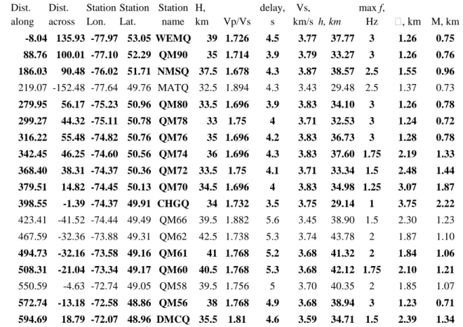
For site WEMQ, these estimates are: crustal thickness from the H-k stack 39 km, 324

Vs = 3.77 km/s; delay of the PmS phase at the highest frequency 4.5 s; thickness estimate

325

using the PmS delay h = 37.77 km; highest frequency f=3 Hz; shortest wavelength

326

Vs/f=1.26 km; Moho width using a formula from Levin et al. (2016) is M~0.75 km. 327

For site D60A, the estimates are: Vs = 3.57 km/s, H= 41.5 km, h=45.38 km, f=0.5 Hz, 328

 7.14 km, M~3.95 km. 329

330

Two estimates of crustal thickness, H and h, differ in the amount of data included 331

in them, and consequently in the volume of the crust that they represent. The H-k stack 332

measure is based on the analysis of the full RF wavefield. An assumption inherent for this 333

measure is that the crust is an infinite uniform layer with a horizontal boundary. 334

Consequently, we construct an omni-directional epicentral gather of all RFs (e.g., Figure 335

3B), and search for H and k values that would best predict positions of positive and 336

negative pulses within it. To insure stability of the stacking procedure, the frequency 337

range of RFs used in this analysis is relatively low, up to 0.5Hz. Because of the 338

directional averaging, the H-k stack measure represents a sample of the crust-mantle 339

boundary depth in a cone circumscribed by all incoming waves. For typical values of 340

incidence angles of direct P-to-S converted waves (Figure 2) this area is approximately 341

30 km in diameter when the crustal thickness is on the order of 35 km, and larger for 342

thicker crust. Multiply-reflected waves included in the H-k stack sample a region 343

approximately twice as wide. Significantly, the stacking procedure is not guided to 344

recognize specific phases in the RF wave field, treating all values as meaningful. As we 345

will discuss in the following section, RF wavefields may be quite complex, with 346

additional phases present in the time interval searched the H-k stack algorithm. This 347

inevitably leads to broad ranges of k values yielding very similar solutions. 348

The crustal thickness measure h using a narrow beam of RFs for a chosen direction 349

samples an area of the crust-mantle boundary a few km across. The use of the same 350

earthquake source region for all estimates using the PmS phase ensures that results are

351

compatible between different locations along our transect. This measure also assumes the 352

crust to be uniform in properties, although the assumption only needs to be true along the 353

RF beam. The estimate of the PmS phase timing is done using the highest frequency of the

354

RF beam that displays a pulse with the shape expected from a simple boundary. In most 355

cases this frequency is much higher than the 0.5Hz used in the H-k stack analysis, and 356

consequently the positioning of the peak of the PmS pulse is clearer (e.g., Figure 4A, sites

357

WEMQ and DMCQ). The PmS estimate of crustal thickness relies on the value of Vp/Vs

358

obtained using the H-k stack, and thus in cases where k is poorly constrained by the H-k 359

stack method, the PmS based estimate is also less reliable. Such instances are discussed

360

individually in the following sections. 361

362

4.4 Glossary of crustal parameters 363

Vp, Vs – average velocities of P wave and S wave in the crust;

H – an estimate of the crustal thickness based on the stacking of direct and

multiply-365

reflected P-to-S converted waves; 366

k – an estimate of the Vp/Vs ratio based on the stacking of direct and multiply-reflected

367

P-to-S converted waves; 368

h – an estimate of the crustal thickness based on the delay time of the P-to-S converted

369

wave PmS and average crustal velocities Vp and Vs;

370

t - the value of the delay time is measured from the hjghest frequency receiver functions

371

preserving a simple shape of the PmS phase.

372

M – Moho width, the vertical distance over which values of seismic velocities change at

373

that bottom of the crust. 374

375

5. RESULTS 376

377

We present a summary of our results in Figure 5, in the form of a composite transect 378

projected onto a line with end points at 79W, 52N and 65.285W, 44.633N. The line is 379

chosen to coincide with the trace of our array where it crosses the Grenville Province, to 380

pass through the Charlevoix region of intense seismic activity in and close to St. 381

Lawrence River, and to be as perpendicular as possible to major tectonic boundaries in 382

the region, such as the Appalachian Front and the Grenville Front (Figure 1). Arguably, 383

our transect traces the shortest path from the oldest rocks in the core of the North 384

American craton to the region of the most recent deformation in the Fundy Basin. Our 385

sites are within ~200 km of the transect trace, resulting in a 400 km wide swath through 386

the continent. All values used to produce Figure 5 are presented in Table 1. 387

388

5.1 Crustal Thickness. 389

Averaged over the length of the profile, our estimates of crustal thickness using the H-k 390

stacking technique yield 37.1+/-2 km, while estimates using picked delay times of PmS

391

phases have an average of 37.0+/-4.6 km. This is very close to 38.3+/-2 km value we 392

obtain by averaging values sampled from the database of Tesauro et al. (2014). 393

394

5.1.1 Grenville Front 395

An increase in crustal thickness relative to the near-constant thickness of the Archean 396

(Levin et al., 2016) and Proterozoic crust is seen on both sides of the GF (Figure 5). 397

From north to south, an abrupt thickening of the crust at the GF is followed by a gradual 398

decrease over a distance of ~150 km (Figure 6). Figure 7 illustrates datasets from three 399

locations adjacent to the GF. An increase in PmS phase delay in excess of 1.5 s takes place

400

between sites QM70 (north of GF, delay of 4 s) and QM66 (very close to the trace of GF, 401

delay of 5.6 s). Delay of 5.3 s is seen at site QM62 south of the GF. All delay values 402

reported here are measured for the chosen highest frequency RF bin (see Methods). At 403

site QM70 an additional positive phase at ~8 s is present, suggesting an additional deeper 404

boundary with strong velocity contrast. Estimates of the crustal thickness are 34.98, 38.9 405

and 43.78 km for sites QM70, QM66, QM62, respectively. We note that the constraints 406

on the value of k are especially weak at site QM66, with nearly all values searched 407

yielding comparable level of “fit”. This is likely due to the poor excitation of crustal 408

multiples that are a key ingredient in the H-k stack. In contrast, at site QM70 multiply 409

reflected P-to-S converted waves may be clearly seen at delays ~13 s (Figure 7), and 410

yield a stable estimate of k. If we choose k=1.75 instead of k=1.88 for site QM66, the 411

estimate of crustal thickness increases to 45.5 km. This estimate would be more 412

consistent with this site having the largest value of PmS phase delay in this part of the

413 transect. 414 415 5.1.2 Appalachian Front 416

The area adjacent to the AF shows a regional increase in the mean crustal thickness. 417

Averaging Moho depth values falling within ~100 km on either side of the AF (between 418

coordinates 700 and 900 km on our transect, Figure 8), we get crustal thickness estimates 419

of 41.44+/3.9 from H-k stacks, and 41.21 +/-4.3 from PmS delay times. An average of

420

values extracted from Tesauro et al. (2014) for the corresponding sites is 39 +/- 0.7 km. 421

Resonances in unconsolidated sediments like those filling parts of the St. 422

Lawrence River valley tend to produce reverberations in RFs (Cassidy, 1992) that 423

complicate their interpretation. Fortunately, sites we use to develop crustal structure 424

constraints in the vicinity of the AF do not display these characteristic features (Figures 425

9, 10, and Supplement). 426

Figure 9 shows examples of H-k stacking surfaces and waveforms for two long-427

running seismic sites on the northern and southern banks of St. Lawrence River (and thus 428

on the opposite sides of the AF). Both sites show evidence for additional structures in the 429

uppermost mantle lithosphere. Site A64 on the northern shore (and thus within the 430

Grenville Province) has a PmS delay of 5.2 s (Figure 9). Combined with the

well-431

constrained low value of k=1.71, this results in a crustal thickness estimate of 44.36 km. 432

An additional positive phase at ~8 s implies a presence of another converting boundary 433

15-20 km beneath the Moho (60-65 km total depth). At site A21 within the Appalachian 434

Orogen the value of PmS delay is larger (5.4 s) while the estimate of the crustal thickness

435

is smaller (37.5 km) due to a very high preferred value of k=1.88. Figure 9 shows that this 436

estimate is not very tight. If k=1.78 (at the lower end of the 5% contour) is chosen for the 437

crustal thickness calculation, we get H=44 km and h=41.75 km. Site A21 also has clear 438

converted phases, positive and negative, at delay times 8-10 s, implying complex 439

structure of the uppermost mantle. 440

While at most sites close to the AF our estimates of crustal thickness approach (or 441

exceed) 40 km, two sites yield very small estimates of crustal thickness (Figure 8). At site 442

A61, on the northern shore of the St. Lawrence River, RF waveforms are complex, and 443

H-k stacking result is poorly constrained. PmS delay value of 5 s was chosen. It is the

444

weaker of the two positive pulses (Figure 10), selected for the proper sense of moveout it 445

displays. It is, however, followed closely by a more energetic pulse at ~6 s, which likely 446

dominates the H-k stack. Consequently, crustal thickness estimates based on the H-k 447

stack (42 km) and the PmS delay (34.5 km) diverge considerably. On the other hand, site

448

E60A displays a simpler wavefield and a well-constrained H-k stack. An estimate of thin 449

crust, H= 32.5 and h=33.3 km, is thus reliable even though this site is an exception for 450

the broad region on both sides of the AF. Notably, this site is near the limit (~200 km) of 451

inclusion into the transect, and thus exemplifies along-strike variability in complex 452

tectonic units crossed by it. 453

5.1.3 Eastern Maine 454

An area with exceptionally small crustal thickness is observed in eastern Maine, between 455

section of the transect are 32.2 +/-1.3 km from the H-k stacks, and 31.6 +/- 1.8 km using 457

PmS delays. For comparison, the average of values sampled from the much more widely

458

spaced grid nodes of Tesauro et al. (2014) are 39.21+/-2.6 km. In Figure 12 we present 459

representative examples of H-k stacks and waveforms for sites within this region, QM16 460

and G64A, that both have thin crust, and also site QM10 where crustal thickness is closer 461

to the regional average. Site QM16 shows clear evidence for thin crust. While the number 462

of records available at this temporary seismic site is relatively small, the H-k stack result 463

is very well constrained, yielding a crustal thickness value of 31 km. The PmS delay of 3.8

464

s yields crustal thickness estimate of 31.9 km. Similarly, site QM10 shows a very well-465

constrained H-k stack result, with a crustal thickness estimate of 34 km. A PmS delay of

466

4.2 s results in crustal thickness estimate of 34.7 km. Sites QM16 and QM10 have near-467

identical best-fitting values of k (Figure 12), thus the change in PmS delay value likely

468

reflects true change in crustal thickness. Site G64A presents a more complicated 469

wavefield, and its H-k stack pattern is less well constrained. There appear to be two 470

patches of near-identical high values on it. The automatically determined best fitting 471

combination is H=26.5 km, k=1.89. Inspection of the H-k diagram (Figure 12) suggests 472

that values of k in 1.7 - 1.8 range offer data fits that are nearly as good. Establishing a 473

maximum value of H-k stack for this range yields a combination H=32, k=1.76 that is 474

more consistent with findings at other nearby sites. A PmS delay value of 3.8 s results in a

475

crustal thickness estimate of 30.51 km. RF waveforms at site G64A contain a clear 476

positive pulse at ~11 s that likely causes a disruption of the H-k stack pattern. The 477

moveout of this pulse in the epicentral RF gather (Figure 12) is consistent with it being a 478

direct converted phase from an interface in the upper mantle. 479

480

5.1.4 Differences between H-k stack crustal thickness and PmS crustal thickness 481

In our dataset and analysis, the values of h and H are almost always different. 482

This is expected as the H obtained by the H-k stack method represents a broader spatial 483

average than h obtained from the PmS value (see Methods section). However, in most

484

cases the difference is within 2 km, and likely reflects the natural uncertainty of these 485

relatively simplistic measures. In instances where H and h estimates agree, we suggest 486

that the similarity is a qualitative measure of simplicity of the crustal structure. 487

Conversely, instances where these values diverge signify crustal and/or upper mantle 488

complexity. Site CHGQ next to the GF is a good example of significant crustal 489

heterogeneity implied by the divergence of H and h (Figure 6). The H-k stack yields a 490

rather unsurprising value of 35 km. However (as discussed in considerable detail in Levin 491

et al., 2016) there is more than one candidate for the PmS pulse in the RF wavefield, and

492

choosing the pulse at 3.5 s delay yields h=29 km. 493

Over the course of our transect we find no systematic relationship between the 494

difference in H and h and any of the other parameters we have constrained (such as Moho 495

width, k), or the tectonic unit. This local nature of complexity reflected in the occasional 496

divergence of simple measures of crustal thickness offers a cautionary note, especially for 497

the extensively used H-k stacking method. Consequently, the summary map showing all 498

crustal thickness values along the transect (Figure 14) depicts h. We believe it to be a 499

more reliable indicator of lateral changes in crustal thickness. 500

501

5.2 Vp/Vs ratio 502

503

A vast majority of sites yields estimates of Vp/Vs ratio (k) that fall between 1.7 and 1.8 504

(Figures 5, 15). Averaging over the entire data set, we obtain k=1.77+/-0.06. A number of 505

solitary outliers are seen, as well as a region of consistently elevated values in the vicinity 506

of the AF. 507

Within the Superior Province two prominent outliers are sites QM66 and MATQ. 508

Both display H-k stack patterns that allow a broad range of values for k that would yield 509

similarly good fits to the waveforms (see Figure 7 for QM66 data). Similarly, site QM39 510

in the Grenville province, and sites QM34 and QM31 in the Appalachian Orogen (see 511

Table 1) have high values of k chosen by the algorithm out of a broad range of nearly-512

identical data fit results. 513

In the vicinity of the AF we also find a number of sites with high, but poorly 514

constrained k values, such as A61 (Figure 10). Better-constrained results are seen at A21 515

on the southern shore of St. Lawrence (Figure 9). Site A54 across the river from it has a 516

very similar pattern. However, in both cases, the range of k values within 5% of the 517

maximum is quite broad, and reaches transect-average value of 1.77. 518

A number of sites display error surfaces that suggest bi-modal distributions of 519

preferred H-k combinations. Figure 13 shows data for two such sites. In both cases there 520

are two regions with stack value within 5% of absolute maximum. RF wave fields are 521

complex, especially at site A11 where, like at all other St. Lawrence River sites, deeper 522

interfaces in the upper mantle are likely. The choice of the best-fitting H-k combination 523

is likely influenced by these additional signals, and ends up being very low (1.70) at A11, 524

and relatively high (1.86) at QM36. Error surfaces suggest, however, that alternative 525

choices are possible for both sites. 526

One location where the high value of k appears to be required by the data is site E60A 527

(Figure 10) where the RF wavefield is simpler, and the shape of the H-k stack surface 528

suggests good constraints on the preferred value. This site, however, is unique in the 529

region, and is located nearly 200 km off of our transect line. 530

531

5.3 Moho Width 532

An estimate of the vertical extent of Moho width on the basis of the wavelength of 533

PmS phases depends on both the frequency of the pulse and the value of k. Given the 534

range of plausible values for k, the wavelength influence dominates. A choice of the 535

wavelength is done on the basis of inspection of frequency-dependent RF beams. As 536

discussed in the Methods section, we seek the highest frequency for which the 537

appearance of the PmS pulse still resembles a converted wave from a single boundary.

538

Figure 4А illustrates the range of observations. In the ideal data set from site WEMQ 539

within the Superior Province we observe a progressive narrowing of the pulse for each 540

successive increase in frequency, and choose the highest frequency our data contain, 3 541

Hz. Most locations in the Superior Province show similar results, yielding estimates of 542

the Moho width not exceeding 1.5 km (Levin et al., 2016). One exception is the area just 543

north of the GF. 544

A major change takes place within the Grenville Province, a short distance north of 545

the St. Lawrence River (Figure 6). A large fraction of sites in the southern half of our 546

transect have estimates of the Moho width in the 3 – 4.5 km range. This is due to 547

observed complexity of PmS pulses at high frequencies, which makes it necessary to

548

choose longer wavelength for estimating the width of the Moho. Figure 4a shows 549

examples of choices made for sites with different degree of complexity in the PmS pulse.

550

Figure 14 shows estimates of crustal thickness and Moho width on a map of the 551

region. There is no obvious correlation between crustal thickness and Moho width in our 552

dataset. There is, however, a strong trend of increasingly variable Moho width with 553

distance away from the Superior Craton (Figure 6, and discussion below). 554

555

5.4 Summary of key results 556

557

 We find locally thickened crust beneath the GF (Figure 6), a region of complex 558

crust and upper mantle on both sides of the AF (Figure 8), and a region of 559

significantly thinned crust in eastern Maine (Figure 11). 560

561

 Throughout the region the ratio of compressional and shear wave speeds k largely 562

stays within the range 1.71 to 1.83 (Figures 5, 15). Close inspection of locations 563

where it exceeds 1.85 reveals broad ranges of acceptable k values at most of them, 564

making this value less reliable. 565

566

 Superior and Grenville Provinces have uniformly small values of Moho width, 567

mostly less than 1.5 km (Figures 5, 14). The few exceptions include regions of 568

intense tectonism: the GF, and the St. Lawrence rift. Within the Appalachian 569

Orogen, the Moho width varies considerably. While instances of sub-km Moho 570

boundary are present, many sites show much wider transitions, up to 4.5 km. 571

572

 In a number of locations, especially close to the boundaries of major tectonic 573

domains (GF, AF) we find compelling evidence for discontinuities in seismic 574

properties that reside below the one that we interpret as the crust-mantle boundary 575

(Figures 6, 8). Commonly observed within the lithospheric upper mantle of 576

Earth’s continents, these features likely reflect its complex history. 577

578

6. DISCUSSION 579

580

6.1 Comparison of our results with other estimates of crustal thickness in the region 581

582

6.1.1 Match and mismatch with Tesauro et al. (2014) 583

We used the continent-wide compilation of Tesauro et al. (2014) as a reference for the 584

value of Vp in our region. To compare the crustal thickness estimates we have obtained 585

with those contained in the 1°x1° grid of Tesauro et al., (2014), we interpolated the 586

values and sampled the resulting surface (Supplementary Figure 1, Table 1) at locations 587

of our sites. Perhaps unsurprisingly, we find significant differences between our estimates 588

of crustal thickness and the interpolated values of Tesauro et al. (2014). We also found a 589

number of locations where our results match well. 590

In the central Superior Province, our estimates of crustal thickness are 591

considerably smaller, while in the southern part (250-400 km along the profile, Figures 5, 592

6) our estimates and those of Tesauro et al. (2014) are similar. South of the GF, where we 593

document a local thickening of the crust, our results diverge again. In most locations 594

where we have reliable results in the vicinity of the St. Lawrence river our estimates of 595

the crustal thickness differ from Tesauro et al. (2014). Finally, almost all sites in the 596

Appalachians have crustal estimates considerably smaller (up to 8 km) than those in the 597

Tesauro et al. (2014) compilation. 598

The differences we see are expected, as the values in a Tesauro et al. (2014) 599

database are compiled from studies using P waves in the crust and the upper mantle 600

immediately beneath it. Most of the observations used are from central and western parts 601

of the North American continent, and their extrapolation into eastern North America is 602

performed on the basis of similarity between tectonic units. Notably, there are data points 603

in Tesauro et al. (2014) for the southern Superior Province region crossed by our profile, 604

and the agreement with our results is best here. 605

The disagreement in crustal thickness values raises the question of the viability of 606

using Vp estimates from Tesauro et al. (2014) as the basis for our own measurements. 607

However, the value we adopt (Vp=6.5 km/s) is a commonly assumed average continental 608

crust value, similar to a global average (Vp=6.45, Christensen and Mooney, 1995). 609

Levin et al. (2016) document tests of the influence of significantly larger and smaller 610

values of Vp on the outcomes of H-k stacking analysis. Changes in Vp on the order of 5% 611

(e.g., from 6.5 km/s to 6.2 km/s for the whole crust) result in systematic changes to H on 612

the order of 2 km. Changes in k are less systematic, and range from negligible to ~0.02 613

(e.g., from 1.75 to 1.73). 614

6.1.2 Other studies employing the H-k method 616

Some of the sites examined in this study are included in the Earthscope Automated 617

Receiver Survey (EARS, IRIS DMC (2010)), a routine data analysis product that uses a 618

version of the H-k stack algorithm (Crotwell and Owens, 2005). Two sites (MATQ and 619

CHGQ) are in the Superior Province, while the rest are in the southernmost Grenville 620

Province around the St. Lawrence River, and in the Appalachians. With few exceptions, 621

our results on the crustal thickness agree with those in the EARS database to within 3 km. 622

Given the likely tradeoffs associated with choices of Vp (a uniform value in our study, a 623

site-specific value in EARS) we feel that this is an expected level of mismatch. A few 624

sites show crustal thickness differences in excess of 10 km. All of them are close to the 625

St. Lawrence River, an area where we see highly complex RF wave fields. Another site 626

with a mismatch of 8 km is on the shore of the Fundy Basin. Similarly, most sites where 627

comparisons are possible have values of k that match to within 0.05. Exceptions once 628

again include sites next to St. Lawrence River, and also site MATQ in the Superior 629

Province (Figure 6) where our result is highly uncertain. 630

A study by Thompson et al., (2015) using another variant of the H-k methodology 631

included three sites we have investigated (WEMQ, MATQ and CHGQ, Figure 6). Near-632

identical results were obtained at WEMQ and MATQ, while for site CHGQ, where we 633

noted considerable complexity in the RF wavefield, Thompson et al. (2015) find a 634

significantly higher value of k. 635

Finally, a recent study by Petrescu et al. (2016) included a limited subset of data 636

used here, and also employed a variant of the H-k stack method to probe average crustal 637

properties. Comparing the values for all locations where Petrescu et al. (2016) had more 638

than 20 records in their analysis, we find very similar results everywhere except at site 639

MATQ in the Superior Province and site A64 on the shore of the St. Lawrence River. In 640

both instances, Petrescu et al. (2016) report ~3 km thicker crust, and smaller values of k. 641

642 643

6.2 Variability of Moho Width 644

645

Based on a subset of the data used here, Levin et al. (2016) noted that all stations 646

within the Superior Craton display uniformly sharp (<1.5 km vertical thickness) Moho 647

transitions regardless of the age of the tectonic terrane or the surface lithology. 648

In the significantly expanded dataset presented here, we observe a similar “baseline” 649

Moho width of less than 1.5 km throughout all tectonic regimes investigated (Superior 650

Province, Grenville Province, and Appalachians), however, there is significantly more 651

variability within the Appalachian terranes as compared with the others (Figures 5, 14, 652

16). Below we highlight two regions where Moho width is seen to deviate significantly 653

from the <1.5 km baseline value: at the Grenville Front and throughout the 654

Appalachians. 655

656

6.2.1 The Grenville Front 657

As noted above, the 1.1 – 0.9 Ga Grenville orogeny is considered to be a period of 658

intense mountain building and deformation due to continent-continent collision, similar 659

to that of the modern-day Himalaya. Despite this tectonic history and surface exposure, 660

there is only a small, laterally restricted, cluster of stations that display slightly more 661

diffuse Moho boundaries, up to 2.5 km thick (Figures 5, 6) immediately adjacent to the 662

Grenville Front in both the Superior Craton and within the parautocthonous Grenville 663

terranes. Away from this small region, Moho width returns to the baseline of <1.5 km 664

throughout the remainder of the Grenville Province, despite the larger mean crustal 665

thickness (as described above). 666

There are two potential causes for this small, laterally-restricted, perturbation of 667

the Moho boundary at the Grenville Front: 668

(1) The accretionary style of the Grenville orogeny. While the Grenville Front 669

was previously suggested to be a vertical tectonic suture (e.g. Dewey and Burke, 1973), 670

there is considerable evidence that the parautochthonous and allochthonous terranes of 671

the Grenville Province may have been thrust at low angle on top of the existing passive 672

margin of the Superior Craton (see Rivers et al., 2015 for a detailed discussion). In this 673

case, the Moho boundary may not be indigenous to the Grenville, but is rather the 674

Archean-age Moho of the pre-existing lithosphere. As such, it would not be expected to 675

have a radically different signature from that of the Superior Craton to the northwest. 676

The small perturbation of ~+1.0 km in Moho thickness at the Grenville Front may 677

be due to the transition from thin Superior Craton crust (average ~35 km) to the relatively 678

thicker crust in the Grenville Province (average ~40 km). The Moho at this transition 679

between thinner and thicker crust may be more diffuse due to lithospheric flow or 680

tectonic suturing at this boundary. 681

(2) An additional explanation of the smaller-than-expected perturbation in Moho 682

width at the Grenville Front may lie in its age. The uniform crustal thickness and sharp 683

Moho transition seen throughout the data from the Superior Craton led Levin et al. (2016) 684

to conclude that the lower crust and lithosphere of the Superior Craton had experienced 685

some degree of delamination and/or reorganization after amalgamation of the craton from 686

numerous continental fragments (terranes). Levin et al. (2016) suggested that the high 687

mantle potential temperatures (and therefore Moho and ambient mantle lithosphere 688

temperature) present during the Archean significantly reduced the viscosity of the crust 689

and lithosphere allowing for efficient reorganization to occur. 690

In the case of the 1.1-0.9 Ga Grenville orogeny, however, mantle potential 691

temperatures are estimated to have been only 100-150°C hotter than the modern day, as 692

compared with ~250°C in the Archean. It is possible that the lower mantle potential 693

temperature, and the limited amount of time since orogenesis, have resulted in the 694

preservation of the Moho perturbation at the Grenville Front today. It is certainly clear 695

when comparing with the more recent deformation history of the Appalachians that there 696

is a strong correlation between increasing Moho width and the timing of tectonism. 697

Fischer (2002) noted the age dependence of the ratio between surface topography and the 698

underlying crustal thickness in continental collision belts, hypothesizing that long-term 699

cooling and attendant metamorphic reactions lead to the loss of buoyancy in the crustal 700

root of the mountains. Age-dependent variations in Moho width documented here likely 701

reflect similar processes. 702

703

6.2.2 Appalachian Front 704

In contrast to the Superior Craton-Grenville Province transition, the transition 705

between the Grenville Province and the accreted terranes of the Appalachians is 706

associated with a large variability in Moho width. As before, the baseline of <1.5 km 707

Moho width is recorded throughout the Appalachian continental crust; however, many 708

stations have Moho width in excess of 4.5-5 km (Figure 8). 709

The ribbon continents of Dashwoods, Ganderia, Avalonia, and Meguma accreted 710

to the Laurentian margin during the Taconic, Salinic, Acadian, and Neoacadian 711

orogenies, causing an eastward migration of the continent boundary. The Dashwoods 712

crustal block is likely underlain by Grenvillian basement (van Staal et al., 2007); whereas 713

Ganderia and Avalonia likely have the Gondwana continental margin at the base (van 714

Staal et al., 1996). Meguma is preserved only in southern Nova Scotia, to the northeast 715

of our seismic profile. 716

Each of these continental fragments has arc-related geochemical affinities, and the 717

accretion of Ganderia and Avalonia in particular led to significant subduction-related 718

volcanism on the western edge of the growing Laurentian margin. Modern day arcs are 719

characterized by highly diffuse Moho boundaries (e.g. Calvert et al., 2008), and thus it is 720

perhaps unsurprising that the continental crust below the Appalachians retains this diffuse 721

Moho signature in many locations. 722

Perhaps most significantly, however, the transition from a uniformly sharp Moho 723

to a more diffuse and variable Moho occurs at locations immediately to the NW of the St. 724

Lawrence River (Figures 8, 16), and is not exactly coincident with the Appalachian Front 725

separating the Proterozoic Grenville Province lithologies from the Phanerozoic 726

Appalachian terranes. The observation of diffuse Moho within the Grenville Province 727

and extending within the Appalachians therefore suggests that the Moho in this region 728

was disturbed prior to the formation of Pangea and the amalgamation of these tectonic 729

fragments. Our results indicate that perhaps the Moho was disturbed during the initial 730

rifting of Rodinia (approximately 765-680 Ma; Ernst and Bleeker, 2010) and the opening 731

of the Iapetus ocean basin, and has since been unable to recover its original sharp 732 structure. 733 734 6.2.3 Concluding statement 735

Our data suggest that the Moho width of 1.5 km or less is a common value within 736

the continental crust, and deviations up to 4.5 or 5 km can result from a variety of 737

tectonic processes affecting the deep crust and lithosphere. Our results suggest that the 738

Moho will become significantly more diffuse during continental rifting episodes, both 739

successful (such the opening of the Atlantic) and not (e.g., the St. Lawrence Rift). 740

Instances of diffuse Moho in the Appalachians imply that in the last ~750 Ma of Earth’s 741

history other tectonic processes (e.g. subduction) may have acted to increase Moho 742

width, and that the time since these episodes have not been sufficient to re-establish the 743

“sharp” Moho seen in older terranes such as Grenville. 744

745

6.3 Crustal properties along a densely sampled continental transect – an overview. 746

747

Maps of our results presented in Figures 14 and 15 and an annotated cross-section (Figure 748

16) offer a broad overview of the crustal properties in three distinct tectonic domains. 749

750

The Superior Province is characterized by a thin crust, sharp Moho and low 751

values of Vp/Vs ratio. While these are expected findings for a region of Archean crust, 752

the uniformity of properties across a large area that includes terranes with distinct 753

histories is notable. Relatively small lateral spacing of our observations, especially in the 754

southern part of the Superior Province, excludes the possibility of local variations being 755

missed. Our study supports the notion that the crust of the Archean continents is indeed 756

very similar, and has a simple internal structure, almost everywhere. This in turn 757

comports well with the narrative of the Archean crust formation involving repeated 758

reworking by density sorting processes (Johnson et al., 2014; Jagoutz and Kelemen, 759

2015; Levin et al., 2016). 760

761

The Appalachian Orogen presents a dramatically different set of traits. All 762

parameters (crustal thickness, Moho width, Vp/Vs ratio) vary broadly over distances of 763

100 km or less, however major tectonic boundaries of the Appalachians (marked in 764

Figures 1, 15, 16) do not have a clear manifestation in the crustal properties. The 765

variability of crustal thickness appears to be systematic, with areas beneath westernmost 766

Appalachian terranes having thicker crust than those along the Atlantic coast. Western 767

parts of the Appalachian Orogen are likely underlain by the Grenville-age passive margin 768

(e.g., Hynes and Rivers, 2010), and thus thick crust beneath them may be at least partially 769

inherited from the passive margin of Laurentia. The dramatic crustal thinning (from over 770

45 to under 30 km) appears to peak in the vicinity of the Norumbega Fault Zone, a 771

complex deformation belt where large amounts of shear deformation took place in the 772

late stages of the Appalachian Orogen formation (Wang and Ludman, 2004). 773

In contrast to the systematic changes in crustal thickness, measures of Moho 774

width and Vp/Vs ratio vary as much across the strike of the Appalachian terranes as they 775

do along it. An area of consistently elevated Vp/Vs ratios is observed adjacent to the St. 776

Lawrence River. Thick crust and complex structure of the crust-mantle transition (Figure 777

8) are consistent with consequences of the late-Proterozoic failed rifting episode (such as 778

the crustal underplating by heavy residues of rifting-related melting, e.g., Ernst and 779

Bleeker, (2010)). 780

781

The Grenville Province presents an intermediate picture, with some crustal 782

thickness variation, and near-uniform values of Vp/Vs and Moho width (Figures 15, 16). 783

Of the three tectonic domains in the region, the Grenville Province has the thickest crust. 784

Vp/Vs ratios are systematically higher than in the Superior Province. Differences 785

between the Grenville Province and the adjacent Superior Province follow the patterns 786

documented by Thompson et al (2010) elsewhere in Canada, and by Yuan (2015) in 787

Australia. The change in crustal thickness across the GF is abrupt on the Superior 788

Province side and more gradual on the Grenville Province side. 789

Sites in the southernmost part of the Grenville Province, adjacent to the St. 790

Lawrence River, display combinations of properties (especially thick crust, diffuse Moho, 791

high Vp/Vs ratio) very similar to those seen on the other side of the Appalachian Front, 792

and consistent with consequences of the failed rifting episode. 793

794

Taken together, our transect presents a view of the Earth’s continental crust as fairly 795

uniform within regions of common tectonic history (Superior, Grenville, Appalachians), 796

with deviations largely limited to major tectonic boundaries. Significantly, of the three 797

tectonic boundaries crossed by our transect, only two have clear manifestations in the 798

crustal structure. The GF is associated with a change in crustal thickness and crustal 799

composition (as reflected in Vp/Vs ratios), while the Norumbega Fault Zone is at the 800

apex of the regional thinning of the Appalachian crust. Interestingly, the most clear 801

tectonic boundary in the region, the Appalachian Front, appears to coincide with the 802

locus of crustal complexity resulting from prior tectonic episodes, and thus presents a 803

clear example of tectonic inheritance over successive Wilson Cycles. 804

805

ACKNOWLEDGEMENTS 806

This work was supported by the NSF Earthscope grant EAR-1147831 and the Aresty 807

Center for Undergraduate Research, and made possible by the open data policies of the 808

Canadian National Data Centre for Earthquake Seismology and Nuclear Explosion 809

Monitoring, and IRIS DMC. Discussions with A. Hynes, and formal reviews by D. Eaton 810

and A. Frederikson contributed greatly to the quality of the paper. Figures were drawn 811

using GMT (Wessel and Smith, 1991). 812

REFERENCES CITED 814

815

Aktas, K., Eaton, D.W., 2006, Upper-mantle velocity structure of the lower Great Lakes 816

region: Tectonophysics, 420, 267–281 817

818

Alcock, F.J., 1945. Logan’s Fault: Journal of the Royal Astronomical Society of Canada, 819

Vol. 39, p.213. 820

821

Ammon, C.J., 1991, The isolation of receiver effects from teleseismic P waveforms: 822

Seismological Society of America Bulletin, v. 81, p. 2504–2510. 823

824

Anovitz, L. M., and E.J. Essene, 1990, Thermobarometry and pressure-temperature paths 825

in the Grenville Province of Ontario: Journal of Petrology 31.1, pp.197-241. 826

827

Artemieva, I.M., 2006, Global 1°x1° thermal model TC1 for the continental lithosphere: 828

implications for lithosphere secular evolution: Tectonophysics, 416, 245-277. 829

830

Bostock, M. G., 1998, Mantle stratigraphy and evolution of the Slave province: Journal 831

of Geophysical Research: Solid Earth,103, B9 pp. 21183-21200. 832

833

Bostock, M. G., 1999, Seismic waves converted from velocity gradient anomalies in the 834

Earth's upper mantle: Geophys. J. Int. 138, 747-756 835

Card, K.D., 1990, A review of the Superior Province of the Canadian Shield, a product of 837

Archean accretion: Precambrian Res. 48, 99–156. 838

839

Calvert, A. J., S. L. Klemperer, N. Takahashi, and B. C. Kerr, 2008, Three-dimensional 840

crustal structure of the Mariana island arc from seismic tomography: J. Geophys. Res., 841

113, B01406, doi:10.1029/2007JB004939. 842

843

Cassidy, J. F. ,1992, Numerical experiments in broadband receiver function analysis: Bull. 844

Seism. Soc. Am. 82, 1453–1474.

845

Christensen, N.I., Mooney, W.D., 1995, Seismic velocity structure and composition of 846

the continental crust: a global view. J. Geophys. Res. 100, 9761–9788. 847

848

Crotwell, H. P., and T. J. Owens, 2005, Automated receiver function processing: Seism. 849

Res. Lett., 76, 702-708. 850

851

David J., Godin L, Stevenson R, O’Neil J, Francis D., 2009, U–Pb ages (3·8–2·7 Ga) and 852

Nd isotope data from the newly identified Eoarchean Nuvvuagittuq supracrustal belt, 853

Superior Craton, Canada: Geological Society of America Bulletin;121:150-163. 854

855

Dewey, JF and K Burke, 1973, Hot Spots and Continental Break-up: Implications for 856

Collisional Orogeny, Geology; v. 2; no. 2; p. 57-60; DOI: 10.1130/0091-7613 857

Ernst, R.E., W. Bleeker, 2010, Large igneous provinces (LIPs), giant dyke swarms, and 859

mantle plumes: significance for breakup events within Canada and adjacent regions from 860

2.5 Ga to the Present: Canadian Journal of Earth Sciences, 47, pp. 695–739 861

862 863

Fischer, K. M., 2002, Waning buoyancy in the crustal roots of old mountains: J. Geophys. 864

Res. 417 (6892) : 933-936 865

866

Frederiksen, A.W., I.J. Ferguson, D. Eaton, S.-K. Miong, E. Gowan, 2006, Mantle fabric 867

at multiple scales across an Archean-Proterozoic boundary, Grenville Front, Canada: 868

Physics of The Earth and Planetary Interiors, v. 158, pp. 240-263, DOI: 869

10.1016/j.pepi.2006.03.025. 870

871

Green, A.G., Milkereit, B., Davidson, A., Spencer, C., Hutchinson, D.R., Cannon, W.F., 872

Lee, M.W., Agena, W.F., Behrendt, J.C., and Hinze, W.J. 1988, Crustal structure of the 873

Grenville Front and adjacent terranes: Geology, 16: 788–792. 874

875

Gurrola, H., and Minster, B.J., 1998, Thickness estimates of the upper-mantle transition 876

zone from bootstrapped velocity spectrum stacks of receiver functions: Geophysical 877

Journal Interna- tional, v. 133, p. 31–43, doi:10.1046/j.1365-246X .1998.1331470.x. 878