Distributed optimization of traffic delay on a periodic switched grid network

Distributed Optimization of Traffic Delay on a Periodic

Switched Grid Network

by

Fabian Ariel Kozynski Waserman

Telecommunications Engineer, Universidad ORT Uruguay, 2011

Submitted to the Department of Electrical Engineering and Computer Science in partial fulfillment of the requirements for the degree of

Master of Science

in Electrical Engineering and Computer Science at the Massachusetts Institute of Technology

September 2013

@

zyv-SARSC e1h N E E MASAIU'ETTS _I-NSTn1TWE .C. .OLOGY

1

Electrical Engineering and

Certified by:

Professor of Electrical Engineering and

Fabiin Kozynski Computer Science August 30, 2013 Lizhong Zheng Computer Science Thesis Supervisor Accepted by: Professor of TLeslie A. Kolodziejski Electrical Engineering and Computer Science Chair, Committee for Graduate Students Department of

Distributed Optimization of Traffic Delay on a Periodic Switched Grid

Network

by Fabian Ariel Kozynski Waserman

Submitted to the Department of Electrical Engineering and Computer Science in partial fulfillment of the requirements for the degree of

Master of Science

Abstract

Given a switched network, e.g. a city grid with semaphores in its intersections or a packet network, each unit (car or packet) accumulates some delay while traversing the network. This delay is undesirable but unavoidable, which makes minimizing the total average delay of the network given certain constraints, a desirable objective.

In this work, we consider the case of periodic networks, meaning that in every traffic cycle inputs to the system are the same and we try to arrive to an allocation of phases in every intersection that minimizes the total delay per cycle.

We propose a model for such networks in which the delay is given as a function of external parameters (arrivals to the system) as well as internal parameters (switching decisions). Additionally, we present a distributed algorithm which makes use of messages passed between adjacent nodes to arrive at a solution with low delay, when compared with what is obtained when nodes take decisions independently.

Furthermore, dealing with large networks proves difficult to arrive to theoretical results. This distributed algorithm gives an insight on how one can analyze big networks by taking a local approach and determining bounds in smaller networks that are part of the big picture.

Thesis Supervisor: Lizhong Zheng

Title: Professor of Electrical Engineering and Computer Science

Acknowledgments

I would like to thank Prof. Lizhong Zheng for his guidance throughout my research. In addition, I would like to acknowledge Prof. Yury Polyanskiy, Prof. Kuang-Cheng Chen, Shao-Lun Huang, Ali Makhdoumi, Kyu Kim and Vitali Abdrashitov for their support and insightful comments while conducting this research and on other topics related to the area.

These past two years at MIT would not have been possible without my friends here. Thanks go to Sunny, German, Andrea, M6nica, Sumit, George, Boris, Dan, Rachael, and many more that have been a steady source of wisdom, entertainment and continuous support. It was my pleasure meeting you and enjoying so many joyful times. Special thanks go to the wonderful people I've worked with at SP during my time living here and which make this community a great place to live in.

Last but not least, I want to thank my friends and family back at home that even though they are far, they feel really close.

Contents

1 Background of road traffic network models and switching policies 1.1 Models for intersections . . . . 1.2 Models and analysis of traffic networks . . . . 1.3 Policy design for switching in intersections . . . . 2 Model of the problem

2.1 Generalities of the model . . . . 2.2 N ode m odel . . . . 2.3 Link m odel . . .. . . . 2.4 D elay m odel . . . . 2.5 Summary of notation . . . . 3 Analysis of the problem

3.1 1-dimensional grid . . . . 3.2 2-dimensional grid . . . . 11 13 13 14 14 17 17 19 19 19 20 21 . . . . 21 . . . . 23 29 . . . . 29 7 4 Simulations of algorithm for 2-dimensional grid

8 CONTENTS

4.2 Simulation of parallel networks . . . . 30 4.3 Simulation of a general network . . . . 32

5 Discussion and future work directions 35

A Simulator 37

Grid indexing . . . . Time diagram example for an intersection . . . . D elay cases . . . .

Diagram of 1-dimensional problem . . . . Delay per node per input in the 2-dimensional case . Total delay in a node . . . .

Delay for random inputs . . . . Delay results for parallel networks . . . . 2 x 2 grid with named nodes. . . . .

List of Figures

Introduction

There are many kinds of networks, for example packet or car networks, where the units experience delay not only due to the time it takes to traverse the links but also due to waiting in the switching nodes. In these nodes, traffic coming from different inputs must be directed to various outputs while the rest of the traffic "waits". This translates into delay.

This delay is unwanted but in most situations it is unavoidable. Because of this, it is important to design clever switching policies for the nodes in order to minimize the delay experienced by the traffic units (cars, packets, etc.). Many policies can be designed and they vary according to how much information from the state of the network they use, as well as their adaptability to change and the locality of their decisions. For example, in the case of car networks, solutions range from simple timed schemes where the traffic light switch on periodic intervals independent of the state of the road, to schemes where the number of cars in the intersections is measured and a central process determines the switching time for a large number of nodes.

All of these policies have their advantages and drawbacks, meaning that new solutions often differ considerably from current ones, depending on the available data as well as the complexity of the solutions that one is seeking. In this paper, we will consider a distributed, adaptable policy that uses little information about the current state of the network, and tries to minimize average delay per node. The fact that the policy is distributed, will allow us to analyze it's effect in localized sub-networks. That way, we can derive results without having to analyze the full network. This is important as similar analysis can be applied to other problems in which large systems are complex but they can be optimized locally.

To accomplish this goal, we will make a few assumptions about our traffic network. Namely, that the system exhibits a periodic behavior and that the system operates in a stable mode, without creating unbounded queues.

The policy will be tested using a simulator based on our assumptions for the network. To determine the performance, we will compare the system to certain benchmark

situations and determine bounds for the performance of similar algorithms in general networks.

Throughout this paper, we will talk about cars to refer to the units and intersections to refer to the nodes. However, these terms can be exchanged by packets and switching devices. The major difference between these two kind of networks is the reaction time (time between switches).

This paper is organized as follows. In chapter 1, past work on the area is summarized, as well as how these approaches led to good solutions or specific problems. In chapter 2, the model and naming convention that will be used in this paper are presented as well as diagrams to understand how some values are measured or calculated. In chapter 3, the model is analyzed theoretically and the algorithms based on the model are introduced here. Different algorithms for different situations are presented, with the more general policy (of which the others are particular cases) is presented in the end. In chapter 4, some of the algorithms presented are simulated in Python (information about the simulator can be found in Appendix A). An analysis of different bounds is also included in this chapter as benchmarks for the simulator, alongside with bounds obtained by analyzing the network locally. Finally, in chapter 5, conclusions about the work are presented alongside with different directions for future work.

Chapter 1

Background of road traffic network

models and switching policies

The problem of traffic networks is one of resource access and allocation. In it, different units (cars) try to access a resource (a stretch of road, an intersection) at the same time while avoiding a collision. Because of this, rules regulating the usage of this medium have appeared and switching mechanisms (traffic lights) are used to provide some kind of fair switching. This signaling introduces delay in those units that must wait for their turn to use the resource; additionally, other questions arise such as the distribution of the units in queues and stability of these queues.

In this chapter, we present the different approaches to this problem that have been taken in the past. We begin with a summary of the different models for a single intersection that have been proposed taking into account different hypothesis. After that, we present the models and analysis applied to traffic networks (more than one intersection). Finally, we present different algorithms and policies that have been proposed to solve or mitigate one or some of the problems inherent to the resource sharing problem applied to road traffic.

N 1.1 Models for intersections

Analysis of traffic models for single intersections can be traced back to the 1950s. In [1] a first analysis of opposing traffic streams is made, and in [2] the distribution of the number of cars waiting at an intersection under certain hypothesis (namely, Poisson arrivals) is determined by the Borel-Tanner distribution presented in [3]. This derivation states that even though an intersection may discharge a queue of cars at a given rate which allows a certain number of cars to pass, a larger number of cars than the expected can pass through the intersection if they don't accumulate in a queue, but arrive to the intersection once it is empty.

In [4,5], the queues formed at a fixed-cycle traffic light are analyzed. They arrive to the lengths of the queues as well as the delay experienced by cars waiting at an intersection as a function of diverse parameters of both the cars' arrivals and the 13

14 CHAPTER 1. BACKGROUND OF ROAD TRAFFIC NETWORK MODELS AND SWITCHING POLICIES

intersection. The results in [4] are compared with observation. However, these are highly dependent on the model utilized for both cars and intersection.

These models present numerous methods to determine the state of an intersection as well as it's output. However, they are highly dependent on the parameters as well as the model chosen. Even though the model may be correct for one intersection, given that the discharge pattern of traffic lights is in no way similar to the arrival pattern (except in the case of a green light with an empty queue), analyzing multiple cascaded intersections cannot be done using the same tools as presented above.

N

1.2 Models and analysis of traffic networks

The interaction between more than one intersection introduces new questions. When considering at least two intersections in tandem, the output of one intersection is the input for the next, and the assumptions about arrivals to it need to be changed (for example, they may not be independent).

In [6], its authors present a model for a city (traffic network) with cars that at every intersection perform a decision about which direction to take based on some probabilistic model. They also analyze the phenomena of dispersal of a platoon of cars as it travels along a road. These factors are the ones that render the hypothesis assumed in the previous section useless after the first intersection.

By utilizing Cellular Automaton [7,8,9] and based in the freeway model presented in [10], models have recently been presented in [11, 12] where the whole network is analyzed at a small scale, with roads and intersections being decomposed into multiple cells, and cars traversing the network following local rules. This kind of models and approaches have been used widely to generate switching policies based completely in local state.

* 1.3 Policy design for switching in intersections

When only one intersection is considered, the problem of switching is clearly local, as there's only one location to take into account. As more intersections are added that relate by the links between them, the problem cannot be decoupled that easily, as the output of one intersection is the input of others. Additionally, the existence of loops (multiple routes from one intersection to another) makes the problem of timing a complex one.

The main question that these papers try to address is the following:

How to determine when different traffic lights in a network should be switched from one state to the next in order to minimize some function of the delay (maximum, average, etc.) in the network?

Sec. 1.3. Policy design for switching in intersections 15

methods. In these papers, their authors determine what is the optimal offset between two intersections set in cascade in order to minimize the delay of cars waiting in the intersections. Even though a result is provided that allows to optimally choose the offset between the switching times via a simple calculation, concatenating more than two intersections using this method is infeasible.

Many mechanisms have been proposed in order to control traffic light scheduling. These include sensor loops at the beginning of the queues to detect presence of cars, to sensor loops in the middle of road links to detect length of queues. Moreover, distributed and centralized algorithms have been deployed in many cities. [15] presents a review of the different mechanisms that have been devised and implemented.

Lately, with the ubiquity of Cellular Automaton in diverse applications as well as with the models presented in [10, 11, 12], policies that operate as Cellular Automaton have been designed. These are distributed policies, and take into account the information that can be sensed directly from the intersection. An algorithm of this kind is presented in [16].

Chapter 2

Model of the problem

In the bibliography, there are numerous models that retain or remove different aspects of the system to simplify calculations or modify hypothesis. To analyze the problem and address the question presented in the previous section, we will simplify the system to a model that we can work with while retaining some of the characteristics of the system as well as maintaining the average delay as a quantity to minimize.

In our model, we will consider a grid of nodes, where cars arrive periodically to each intersection from every direction and after waiting for certain time, they go through the intersection until they reach another one or go out of the system. The quantity to optimize will be the delay that cars experience while traversing the network by waiting at the nodes and the variable to control this is the start of flow of cars for a specific direction for each intersection.

In this chapter we describe the model including the different parameters and variables in it as well as the way that the total delay is obtained from them.

* 2.1 Generalities of the model

The traffic network will be modeled by a grid of nodes (intersections). These nodes are connected in a way that traffic from a node can only go to its immediate neighbors (up, down, left, right). We will consider two cases, 1-dimensional and 2-dimensional. In the first case, we will index nodes by i E {O, 1, ... , N - 1} and in the second case by

(i, j) E

{0, ...

{o,

Traffic can only appear to, and disappear from the network in the nodes around the edge of it. This means that the flow of cars is conserved in every node in the inside of the grids. Additionally, we will assume that traffic does not take turns, that is, cars will always follow the same direction. This means that traffic that appears in one end of a given row in the grid will traverse the grid and go out at the other end in the same row, and similarly for columns.

0,0 1,0 2,0 3,0 4,0 5,0 6,0 0,1 1,1 2,1 3,1 O1 5,1 6,1 0,2 1,2 2,2 3,2 4,2 5,2 6,2 0,3 1,3 2,3 3,3 4,3 5,3 6,3 0,4 1,4 2,4 3,4 4,4 5,4 6,4 0,5 1,5 2,5 3,5 4,5 5,5 6,5

1-dimensional grid 2-dimensional grid

Figure 2.1. Examples of grids an respective indexing in the 1-dimensional and 2-dimensional cases.

At any given time, a node is in exactly one of two states: it is either letting flow go through in the up +- down direction or in the left +-* right.

We will assume that traffic lights follow a periodic pattern. Each cycle of lights will have length 1 in each node, and will be composed of an interval of length p in which traffic flows in the left + right direction and an interval of length 1 - p in which traffic flows in the up ++ down direction. This p is a known parameter equal for all nodes. For a given node and a given direction, we will call the flowing phase the one where traffic in that direction can go through the intersection and the other phase will be called the

blocking phase.

Given this periodicity, all values for variables should be taken mod 1 and differences in time between two points should be taken accordingly.

We will associate a direction d with the motion of cars and messages, according on where they come from. These directions will be d E {W, E, S, N}.

Traffic will approach a given node i periodically from direction d as blocks of tightly packed cars of length Ld(i), meaning that the cars experience no dispersion. This length is measured in time units, meaning that a block of length L will be discharged by a traffic light in time L. The blocks only break apart when stopped by a traffic light.

Figure 2.2 represents a time diagram of an intersection with cars approaching periodically. The figure shows the traffic light pattern, the blocks of cars approaching the intersection (from W, for example), and when cars go through the intersection.

In this model, we make two simplifying assumptions:

1. The system is periodic: cars arrive to the inputs of the system at the same point in the period in every period and lights in every intersection follow a periodic pattern. 2. The system is stable: in every node i, LW, LE p and LN, LS K 1 - p. This

guarantees that no cars accumulate in the intersection from one cycle to the next.

Sec. 2.2. Node model 19 a) b) c) t SL L L L -L t t Figure 2.2. Timing example for an intersection. a) represents the pattern of green and

red light as seen for the W ++ E direction. b) represents blocks of cars of length L arriving periodically at the intersection (from direction W, for example). The left most end is the time the head of the block of cars arrives at the intersection. c) represents how the blocks are split according to when they cross the intersection: the blue cars go through it without any delay, the yellow cars have to wait until the next cycle (the wait time for each car

is the duration of the red phase).

* 2.2 Node model

Every node will have a control variable x(i) E [0, 1) that specifies the start of the W E cycle (we will call it the green cycle). This means that cars can flow in the W - E

direction during the interval [x, x + p) and can flow in the S ++ N direction during the

interval [x + p, x) (everything considered mod 1).

We consider the time that the head of each block of cars arrives at intersection i from direction d as ad(i) with ad(i) E [0, 1).

* 2.3 Link model

We associate with each link a time value which is the time it takes each car to traverse said link. For the link between nodes i and

j,

J).

* 2.4 Delay model

The total delay (per cycle) incurred in a given node i is simply the sum of the delays incurred in that cycle by the cars that wait in each of its inputs. We will call this delay J.

The delay per input per cycle is just the length of the block of cars that have to wait until the next start of traffic flow, multiplied by the time that the first car in the queue has to wait until said start. The expression for this delay takes different forms depending on the relations between x, ad, Ld, p. Three situations can arise:

CHAPTER 2. MODEL OF THE PROBLEM

L L L

t t t

a) delay = rL b) delay = 0 c) delay = rL'

Figure 2.3. Delay in the input of a node for different situations depending on the relation between x, a, L and p.

have to wait until the next flowing phase. Each car in the block will incur a delay equal to the waiting time of the first car of the platoon.

b) If the head of the platoon arrives in the flowing phase and the remaining time is greater than the length of the block of cars, no delay is incurred.

c) If the head of the platoon arrives in the flowing phase but the remaining time is less than the length of the block of cars, those cars that remain incur in a delay whose length is that of the blocking phase.

In Figure 2.3, the three cases are presented with the delay incurred by the platoon in each for a given input. We will call this per node delay 3

d(i), and the total delay in node i per cycle is J(i).

* 2.5 Summary of notation

In Table 2.1 the different variables and parameters are summarized. Notation Meaning

W, E, S, N Directions of traffic or messages. Indicates where it comes from. p Length of the W ++ E phase in the intersections.

Ld(i) Volume of traffic approaching intersection i from direction d.

ad(i) Time the block of cars reaches node i from direction d. x(i) Start time of flow in direction W ++ E in node i.

A(i, j) Travel time between nodes i and j.

6 Total delay in the intersections per cycle.

6(i) Total delay in node i per cycle.

Table 2.1. Notation used for the different variables and parameters.

Chapter 3

Analysis of the problem

In this chapter, we analyze both instances of the problem: the 1-dimensional and the 2-dimensional. For each case, we formulate the problem and proceed to analyze a solution for it.

In both cases, we will analyze traffic moving without encountering opposing traffic. The case of opposing traffic presents the difficulty that its analysis reverses the time line of each node the traffic goes through. We consider the case of cars going East and South.

* 3.1 1-dimensional grid

Assume a linear grid as the one presented in Figure 2.1. We will assume that traffic can only enter the grid from the left hand side and from the North in each node.

As we can take any reference point, assume that aw(0) = 0 and all times are measured with respect to this. Between nodes i and i

+

Figure 3.1 there is an updated version of the diagram.

We will call Lw(0) = L and LN(i) = Li to simplify notation. Using the stability

assumption, we have that L < p and that Li < 1 - p for all i E {0, 1, ... ,N - 1}. For each i, we need to select an x(i) = xi. This means that the respective aw(i) for

aN(0) aN(1) aN(2) aN(3) aN(4) aN(5) aN(N-2)

aw (O)=0

--aw(O)=O 'V O A1 A2 A3 _A4 A5 AN-2 Figure 3.1. Representation of the 1-dimensional grid. Cars enter the grid through the

left and above. The timing reference point is the entry time on the leftmost node from the West direction.

the nodes will be

i) A 0 if i = 0

aw

In the following paragraphs, we will do slight transformations on the parameters and variables to show that there is a relatively easy way of optimizing the delay.

As the Aj are constant, we can change the time coordinates in each node such that the cars arrive to the ith intersection at time aw(i) = E~=' xk. This implies that the cars arrivals to the intersection from the North need to be modified to dN(i) = aN(i) - Ai. Without loss of generality, we can call these new values aN(i) transforming our grid into one with 0 delay between nodes.

In each intersection i, the delay incurred by cars is a function of aw(i), aNi), xi, L

and Li and parametrized by p which is a known parameter. Then, given a function

f

6(i) =

f

k=0

we can transform the time coordinates in this node (note that the delay is independent of other nodes given the Xk values in previous nodes) to obtain

i-1 i-1

6(i) = f Xi - x Xk, 0, aN(i) - Xk, L, LJ =f(a, 0,3, L, Lj)

k=0 k=O

where a and 3 are two independent variables in [0, 1).

Using the breakdown in section 2.4, we have the following expression for 6(i):

6(i)

f(a,

3,

+ aE[1-p,1+L-p)

_{(L -}

_{(a + p}

- p)

_(3.1)

+

+

+ 1 _{a+pe[i3-(1-p),0+Lj-(1-p))}

_{(0 +}

- (a

+

p))

Note that whenever a difference is taken or an interval is considered, the periodic nature of the time line should be taken into account.

We can see that (3.1) is piecewise linear with respect to a and

/

j

* 3.1.1 Optimization of the delay

Our goal is to find the values for xi that minimize the total delay in the system. To do this, we will utilize the function

f

programming.

Let gj (t) be the minimum total delay obtainable between nodes j and N - 1 given that ZjI0 Xk = _{t. Then, we can optimize starting from the last node and going back,}

using the decoupling mentioned previously. In (3.2), the expressions for gj (t) are shown and the optimum delay is simply go (0).

min f(y,t,aN(j),L,Lj) ifj=N-1

gj(t) = _(3.2)

{( min j+_{1(x + y) +}

_f

if 0 < j < N - 2

yE[0,1)

In each step, the optimization is over a piecewise linear function divided by linear constraints in a bounded square. The minimization gives rise to a piecewise linear function (in x) and the argmin is in each case a linear function (it traces the boundaries of the regions). Then, these messages are simple to encode, though may get longer if the network is too big.

In this way, we can find optimal values for xi as well as the optimal delay J. This can be done off-line as well as on-line sending messages backwards.

In each step of the dynamic programming algorithm, the regions may get more complicated while still being a linear optimization. This might mean more discontinuities in each step. Smoothing and weighing gj (x) reduces the impact of these boundaries and attenuates the appearance of more discontinuities, with the cost of losing the linearity of the functions and regions.

* 3.2 2-dimensional grid

As stated before, we will consider the case of no opposing traffic. This means that traffic will only come into the system from the West and from the North.

For this case we will assume that p = I, and L(i, j) = - for all nodes, meaning there is no idle time at any intersection. This assumption is just for simplifying the theoretical analysis.

To simplify the notation, we realize a transformation in the time axis of the form y F y

+

As cars only travel in two directions, nodes will only have aw and aN defined. We will have delays between nodes of the following kind:

* As(i, j) is the delay between nodes (i, j) and (i

+

j).

" AE(i, y) is the delay between nodes (i, j) and (i, j + 1). That is, going West to

East.

24 CHAPTER 3. ANALYSIS OF THE PROBLEM

t t

t L'i' t

a) delay = r b) delay = L'

Figure 3.2. Delay per node per input in the 2-dimensional case with the assumption that p = } and L = .. We can see that the expression of the delay depends on the relationship between a and x, but it always has a factor of .1 In Figure a) cars arrive in the blocking period, and in Figure b) cars arrive in the flowing period.

Then, we have that aw(i,j+1) = _{x(i,j)+AE(i,j) and aN(i+1,j) =}

x(ij)+As(ij)-* 3.2.1 Delay model for a node

Given that there is no idle time in the nodes, calculating the delay for each input, based on the values for a and x is relatively straightforward.

There are two cases for the delay:

a) The head of the block of cars arrive to the intersection in the flowing phase. b) The head of the block of cars arrive to the intersection in the blocking phase.

In Figure 3.2, we can see the delay incurred by cars in each of these cases.

Note that in both cases there is a factor of 1. Given that this factor appears in all nodes in both inputs, we will divide the delay by this factor and not consider in the calculations. This is just a change of scale that obscures only the total value of the delay.

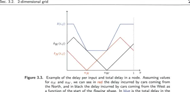
In Figure 3.3 we can see a plot of the delay (without the factor) as a function of the beginning of the flowing phase (x), parametrized by the times the cars arrive to the intersection from each direction.

We will call this function 6(i, j) A

f(x; aw, aN)

N

3.2.2 Parallel network

We define a parallel network as one in which for each i E {0, 1, ... , N - 2}, As(i, j) = As(i) and for each j E {0, 1, ... , M - 2}, AE(i, j) = AE(j). This means that the grid satisfies that any shortest path (in terms of hops) from one node to another has the same delay.

Sec. 3.2. 2-dimensional grid

3(i,j)

aN aW 1 X

Figure 3.3. Example of the delay per input and total delay in a node. Assuming values for aN and aw, we can see in red the delay incurred by cars coming from the North, and in black the delay incurred by cars coming from the West as a function of the start of the flowing phase. In blue is the total delay in the node, as a function of x.

Theorem 3.2.1. In a parallel network, the average delay per node, that is the total

delay divided by the number of nodes, can be made to converge to 0 as the network grows

(N -+ oc, M -+ _{oo) by choosing the appropriate x(i, j).}

Proof. We will show this by proving that for every interior node (i,

j

For this proof we will assume a square network (N = M) but the same proof can

be realized for any network in which N+M -+ 0. Note that this is not true in the

NM

1-dimensional grid.

To accomplish this, we proceed in the following way:

1. Select any value for x(N, N), for example x(N, N) = 0.

2. Determine the values of x(N-1, N) and x(N, N-1) such that aw(N, N) = x(N, N)

and aN(N, N) = x(N, N). Select x(N - 1, N) and x(N, N - 1) according to that.

3. (a) Using the property of parallel networks, we know that there exists a x(N

-1, N-1) such that aN(N, N-1) = x(N, N-1) and aw(N-1, N) = x(N-1, N).

This is because both paths from (N - 1, N - 1) to (N, N) have the same delay. Select that x(N - 1, N - 1).

(b) Select x(N - 2, N) such that aN(N - 1, N) = x(N - 1, N) and x(N, N - 2) such that aw(N, N - 1) = x(N, N - 1).

4. Continue with this procedure going towards the North and West of the grid (along the diagonals), selecting appropriately the values for x in such a way that cars arrive to the next intersection at the moment cars start flowing in that intersection. 25

Notice that this can be done with every node in the interior of the grid consistently, but because aw (i, 0) and aN (0, j) are inputs to the problem, there will always be some delay in those nodes.

We can take a really loose upper bound for the delay of each node as 1 (no group of cars will ever be delayed by a time larger than 2). Then our total delay is 6 ; 2N and

then the average delay per node is bounded by M.

N

3.2.3 Optimization algorithm

In a general network, the above procedure (used in parallel networks) will not work, as different paths will not have the same delay. Moreover, doing an optimization like the one in subsection 3.1.1 does not work because there is no way of providing a consistent ordering for the nodes.

To solve this problem, we will give an iterative procedure that will try to converge to the optimum allocation for x(i, j). This algorithm will proceed in a similar fashion to the one described in subsection 3.1.1 with the difference that, having two inputs in each node, we will fix each one in turn while we optimize on the other.

If the nodes worked independently of each other, looking at Figure 3.3 we can see that the optimal choice is any value between aN and aw. In general, for any independent node, this will be the optimal choice (considering always the shortest interval in the periodic time). However, choices of x in a node determine the values of aN and aw in subsequent nodes. This makes the choice not so obvious, as different values in the segment [aN, awl will produce different results. Moreover, it is possible that by not selecting optimally in a node, we can produce better results in the overall network.

For every node, we want to send a message upstream that quantifies what delay that node will incur in if traffic is sent at a specific time and the node operates optimally with that knowledge. These messages will accumulate the information received from downstream and condense it into one function.

Alongside the function f(x; aw, aN) we define the messages g(i,j) (aw) and h(ij) (aN) as in (3.3) and (3.4) respectively, and taking value 0 when the corresponding nodes do not exist.

g(ilj)(aw) : aw min _X f (x; aW .aN(ij)) + 9(i,j+l) (X + AE (ij)

(3.3)

+ h(i+1,j) (x + As(ij))

h(j,j)(aN): aN - min f (x; aw(ij).aN) + 9(i,j+1) (X AE (i,j))

X _(3.4)

+ h(i+1,j) (x + As(ij))

These two messages are passed to the node immediately to the left and immediately above respectively, and encode the following information:

o The g messages tell the node on its left what the optimum delay will be if the cars

arrive at that intersection from the West with a given aw.

e The h messages tell the node above it what the optimum delay will be if the cars arrive at that intersection from the North with a given

aN-Note that we include the delay between nodes to relate the received message with the corresponding delay function.

Using these messages, a node can determine the optimal choice for x using (3.5). This is accomplished by assuming fixed inputs to the node and utilizing the messages to

include in the optimization the effects of choosing one x over another.

x*(ij) =argmin f (x; aw(i,j), aN(i,)) +9(i,j+i) (X + AE(i,)) h(i+,j) (x + As(i,j)) (3.5)

Then, given values for aw(iO), aN(Oj), AE(i,j) and As(i,j) we have the following iterative algorithm to choose values for x:

1. Start with random values of x for each node and compute the corresponding values for aN and aw for every node.

2. Repeat until "convergence", for every time-step t:

(a) Each node computes gt+l(aw) using a' and ht'+(aN) using aw. Note that these messages are functions [0, 1) --+ R

(b) Using the received messages, determine (in row-major order, for example) the optimal values of xt+1, af+1, and at+1 using (3.5) as well as the delay between nodes.

This algorithm can be run in every node in a distributed way, as each node only needs to measure the arrival times to it. One may question the fact that nodes may need to know about the delays between each other, but this can be solved by sending the current arrival time to the upstream node along with the message. In this way, a

node can calculate the delay to the next node by subtracting it's start time x.

Note that while running this algorithm, the values of x, aN, and aw change on every iteration, affecting the periodicity of the system. We could assume that these changes are small, for example by giving inertia to the change (and changing to the midpoint between xt+1 and xt, instead) or by taking a certain number of cycles to realize the changes.

27 Sec. 3.2. 2-dimensional grid

Chapter 4

Simulations of algorithm for

2-dimensional grid

After defining the algorithm for choosing good values for x(i, j) we want to try it in different grids in order to see how efficient it is.

We can model a grid by having probabilities distributions in the links joining the nodes such that links communicating same pair of rows or same pair of columns have the same distribution. Then, a parallel network is one in which these distributions are deterministic.

In this chapter, we will analyze how the algorithm performs in different cases. To have a reference, we will first consider two cases to use as benchmark: completely random selection of x(i, j), and smart selection of x(i, j) with random input values.

For the simulations, we use a Python script that performs the iterations and the messages defined in subsection 3.2.3. The new x(i, j) is chosen in every iteration as the midpoint of the optimal new value and the old value. This simulator will be described in more detail in Appendix A

N 4.1 Benchmarks

To benchmark the algorithm, we will consider the average delay (per node) in a system in which the arrivals to the node are random. We consider two cases: uniform random selection of x(i,

j)

N 4.1.1 Uniform random selection of x(ij)

In this case, we can get the total expected value of the delay (without the 1 factor) by looking at the delay per input given in Figure 3.3. Given aw and aN, the expected delay per input will be ₄₂and then the expected delay per node is .

If we now consider aw and aN uniform in [0, 1) x [0, 1), we still have an expected delay per node of 1

CHAPTER 4. SIMULATIONS OF ALGORITHM FOR 2-DIMENSIONAL GRID

This benchmark assumes that the nodes share no information among each other and act disregarding any information from the state of the intersection.

* 4.1.2 Smart selection of

x(i, j)

By smart selection we mean that even though the nodes don't communicate with each other, for each value of aw and aN, x(i,

j)

In this case, Figure 4.1 represents the values of the delay according to the values of aN and aw. Taking the average with a uniform distribution in the unit square, we arrive at a total expected delay of 1 per node. We can see that this value is less (better) than in the previous section, as we are making a better choice in each node.

* 4.2 Simulation of parallel networks

In the case of parallel networks, we have Theorem 3.2.1 which tells us that a minimum result can be obtained with 0 delay in all the internal nodes.

If the algorithm defined in subsection 3.2.3 is of any use, it should converge to a solution that is close to this minimum, in terms of delay as well as choice of x(i, j). To verify this, we make use of a Python Script that runs multiple steps of the algorithm.

In all simulations, the values for the delays in every row and every column are chosen independently uniformly at random in [0, 1). Similarly with the inputs aw(i, 0) and

aN(0,j)-aN., --- --- - --- --- --- -- --- --- --- --- (1 , 1) aW+1-aN aN -aW aw-aN aN+l aw aw

Figure 4.1. This figure represent the values of the optimum (minimal) delay that can be achieved according to Figure 3.3 for each possible values of aN and

aw. This minimum is achieved by choosing for x any point in the shortest segment between aN and aw, considering the segment [0, 1) as periodic.

Sec. 4.2. Simulation of parallel networks 31

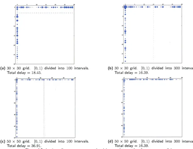
In Figure 4.2 we can see the results of different simulations of a parallel network. The images represent the delay of each node of the network at the end of the simulation

for different values of N = M as well as different discretization of the interval [0, 1).

For each node, a representation of the total delay in that node, with larger circles corresponding to larger delays, the radius being the delay in that node (going from 0 to 1).

We can see that the results obtained comply with those foreseen by Theorem 3.2.1. The total delay is not a good measurement value, since this is dependent on the number of iterations. However, for these cases (750 iterations), the value presented little change per step at the end of the simulation (less than 0.01 per step) and it was diminishing.

(a) 30 x 30 grid. [0, 1) divided into 100 intervals.

Total delay = 18.45.

30

**... 0. -00.0.

(b) 30 x 30 grid. [0, 1) divided into 300 intervals. Total delay = 16.39.

(c) 50 x 50 grid. [0, 1) divided into 100 intervals. (d) 50 x 50 grid. [0, 1) divided into 300 intervals.

Total delay = 36.91. Total delay = 16.39.

Figure 4.2. In these figures we can see the delay per intersection for square parallel networks of sizes N = 30 and N = 50. The delay is represented as a circle

whose radius is equal to the total delay in that node. We can see that, save for small errors (due to numerical errors of the discretization), in all cases the algorithm converges to the expected results, which is almost no delay in the interior nodes and all delay in the input nodes. We see that the end delay is always lower than 2N (and also lower than N). We can see that for higher number of intervals in the partition of [0, 1), the delay is lower.

*.**... ... *... 0..6000 S & 0 0 0 0 0 0 0 0 i

CHAPTER 4. SIMULATIONS OF ALGORITHM FOR 2-DIMENSIONAL GRID

N = M Average delay in 50 runs Average delay per node

10 18.01 0.18 20 68.60 0.17 30 150.14 0.16 40 263.35 0.16 50 407.66 0.16 60 585.49 0.16 70 794.09 0.16 80 1034.83 0.16 90 1304.83 0.16

Table 4.1. Average delay and average delay per node for 50 runs with varying grid size. We can see that the average delay per node is approximately , which is lower than the value obtained by optimizing each node independently. However, this value of is not a theoretical result.

* 4.3 Simulation of a general network

To simulate a general network, we will specify a non-deterministic probability distribution for the link delays.

The simplest case is to assume that all links are I.I.D. uniform in the interval [0, 1). In this situation, one could think that the optimal solution would be the one found in subsection 4.1.2, as the arrivals to every node are uniform in [0, 1). However, this is not true as in the benchmark analysis, we consider just one node but in the algorithm, the information of the delay is used to optimize. Even though the delay is random, once an instance of the problem is selected, the delay is fixed in that instance and the relationship between the timing of the nodes can be used to improve the result of average delay below 1, meaning that the system is making use of the messages to achieve better performances than by just optimizing in each node.

In Table 4.1 we can see the average total delay after 50 runs of the simulator for different grid sizes, as well as the average delay per node. We see that the delay per node obtained is below .

* 4.3.1 Calculation of a lower bound

To calculate an expected lower bound for the delay presented by the algorithm, we will consider a 2 x 2 grid, as seen in Figure 4.3. We are assuming that the major reason why the average delay cannot be brought down to 0 is because the two paths between nodes 1 and 4 present different delays, and this affects every 2 x 2 sub-grid in the general network.

Because of this, the two inputs to node 4 behave as independent inputs. Assuming no delays in nodes 2 and 3, each input is the sum of two uniforms [0, 1). However, due 32

Sec. 4.3. Simulation of a general network ₃₃

1 2

3 4

Figure 4.3. 2 x 2 grid with named nodes.

to the aliasing given by taking mod 1, they both become uniform [0, 1). This means that in this case, the inputs to node 4 will be uniform, giving a delay of -.

This value gives a minimum delay in the 2 x 2 grid of .

One could argue that the large network is not composed of independent 2 x 2 grids, as messages communicate from one to the other. This could lower the bound, but analyzing this effect requires observing larger and larger subnetworks, which is what we are trying to avoid.

Chapter 5

Discussion and future work

directions

In this paper we presented a model for a traffic network (grid) based on the assumptions of periodicity and stability. This model allowed us to develop an algorithm to choose an "optimal" scheduling for the traffic lights in order to minimize the delay incurred by cars

traversing the network.

In the case of a 1-dimensional grid, this solution can be calculated exactly by realizing a series of linear optimizations. These can be realized off-line, providing a solution for the problem as soon as the parameters of the system are known. If an on-line solution is required, the algorithm presented in subsection 3.2.3 can be used.

For the case of the 2-dimensional grid, an iterative algorithm was designed (that can even be applied to cases of a 1-dimensional grid) which tries to locally minimize the delay while taking into account the impact of other nodes. This algorithm performs well, achieving a per node average delay below the benchmark obtained by optimizing each node individually in the case of uniform delays between nodes, and achieving the theoretical result in the case of a network with same delay in parallel links.

The information that each node needs to sense as well as the messages that it needs to pass on is considerably low. Each node only needs to receive messages, compute the new ones and send them upstream, as well as calculate its optimum value. This makes it a true distributed algorithm that can be implemented easily in each node.

Given the results obtained we see that we can optimize the delay by running local optimizations that yield a good per node value, at least when compared to the naive method of optimizing each node.

This distributed algorithm presents the additional advantage that it can adapt to changes in the inputs of the system, given that it starts by assigning a random solution when it starts and then propagating the information of the inputs through all the nodes affected by them. However, this may take a considerable number of time steps as the network grows larger.

As networks grow large, it is important to be able to bound the performance of

36 CHAPTER 5. DISCUSSION AND FUTURE WORK DIRECTIONS the algorithm and analyze the network via local approximations. Because of this, we developed a series of local bounds that allow us to determine the performance in a big network by trying to optimize smaller subnetworks.

In the future, the effectiveness of this algorithm could be analyzed when using non-uniform distributions for the delay within nodes. This will make it possible to bound and estimate the results that can be obtained in more classes of networks. Additionally, the algorithm can be redesigned to accommodate networks that are not grids, though it will require to develop a model on how the cars choose what path to take at each intersection.

Appendix

A

Simulator

The simulator is composed of a Python script that reproduces the algorithm presented in subsection 3.2.3. The script is able to simulate grids of any size, with any kind of distribution for the delays between the links as well as the inputs for the nodes where cars enter the system.

To be able to create, pass on and minimize the functions, the time interval [0, 1) is discretized into uniform intervals. The script allows to specify how many intervals are required, with the only constraint that this is an even number.

The simulator works in a distributed way, with every node calculating its own messages, passing them on and optimizing their delay function. The global control just iterates over every node and assigns the values of the inputs to the nodes (time of the head of the platoon) by observing the previous nodes' switching time (x) as well as the delay between nodes. Note that in reality, this value is not calculated by the nodes, but it's just the result of the cars going from node to node.

To address the fact that the system doesn't maintain its periodicity in each step, the new switching time (xt+1) is not the optimum value as calculated by (3.5), but it is the midpoint (using the shortest segment in the circle [0, 1)) between that value and the old value x.

Bibliography

[1] J. C. Tanner. A problem of interference between two queues. Biometrika, 40(1/2): pp. 58-69, 1953. ISSN 00063444. URL http: //www.

jstor.

ISSN 00063444. URL http://www.

jstor.

[3] Frank A. Haight and Melvin Allen Breuer. The borel-tanner distribution. Biometrika,

47(1/2):pp. 143-150, 1960. ISSN 00063444. URL http: //www. j stor. org/stable/

2332966.

[4] A.J. Miller. Settings for fixed-cycle traffic signals. OR, pages 373-386, 1963. URL http: //www.

jstor.

[5] G.F. Newell. Queues for a fixed-cycle traffic light. The Annals of Mathematical

Statistics, 31(3):589-597, 1960. URL http: //www.

j

Trans-portation Research, 12(2):121 - 130, 1978. ISSN 0041-1647. doi: 10.1016/

0041-1647(78)90051-5. URL http: //www. sciencedirect. com/science/article/

pii/0041164778900515.

[7] J. Von Neumann and A.W. Burks. Theory of self-reproducing automata. 1966. [8] S. Wolfram. Statistical mechanics of cellular automata. Reviews of modern physics,

55(3):601, 1983.

[9] 0. Martin, A.M. Odlyzko, and S. Wolfram. Algebraic properties of cellular automata.

Communications in mathematical physics, 93(2):219-258, 1984.

[10] Kai Nagel and Michael Schreckenberg. A cellular automaton model for freeway traffic. J. Phys. I France, 2(12):2221-2229, 1992. doi: 10.1051/jpl:1992277. URL

http://dx.doi.org/10.1051/jpl:1992277.

[11] S. Maerivoet and B. De Moor. Cellular automata models of road traffic. Physics

Reports, 419(1):1-64, 2005. URL http: //arxiv.org/pdf/physics/0509082.pdf.

[12] T. Neumann and P. Wagner. Delay times in a cellular traffic flow model for road sections with periodic outflow. The European Physical Journal B, 63:255-264, 2008. ISSN 1434-6028. doi: 10.1140/epjb/e2008-00234-6. URL http: //dx. doi. org/10.

1140/epjb/e2008-00234-6.

[13] A.J. Al-Khalili and C.J. Macleod. Derivation of an expression for the optimum offset between two adjacent road junctions using regression analysis. Transportation

Research, 9(6):355 - 362, 1975. ISSN 0041-1647. doi: http://dx.doi.org/10.1016/

0041-1647(75)90006-4. URL http: //www. sciencedirect. com/science/article/

pii/0041164775900064.

[14] Asim J. Al-Khalili, Afifi H. Soliman, and Attahiru Sule Alfa. A model for optimum offset between two signalized intersections. Transportation Planning

and Technology, 11(2):149-162, 1986. doi: 10.1080/03081068608717337. URL

http: //www .tandf online. com/doi/abs/10. 1080/03081068608717337.

[15] M. Papageorgiou, C. Diakaki, V. Dinopoulou, A. Kotsialos, and Yibing Wang. Review of road traffic control strategies. Proceedings of the IEEE, 91(12):2043 -2067, dec 2003. ISSN 0018-9219. doi: 10.1109/JPROC.2003.819610.

[16] Jan de Gier, Timothy M Garoni, and Omar Rojas. Traffic flow on realistic road networks with adaptive traffic lights. Journal of Statistical Mechanics: Theory and

Experiment, 2011(04):PO4008, 2011. URL http://stacks.iop. org/1742-5468/

2011/i=04/a=PO4008.