World Urbanization Prospects: an alternative to the UN model of projection compatible with urban transition theory

D

OCUMENT DE

T

RAVAIL

DT/2004/08

World Urbanization Prospects:

an alternative to the UN model of

projection compatible with urban

transition theory

WORLD URBANIZATION PROSPECTS:

AN ALTERNATIVE TO THE UN MODEL OF PROJECTION COMPATIBLE WITH URBAN TRANSITION THEORY1

Philippe Bocquier DIAL - UR CIPRÉ de l’IRD

bocquier@dial.prd.fr

Document de travail DIAL / Unité de Recherche CIPRÉ

Octobre 2004

ABSTRACT

This paper proposes to critically examine the United Nations projections on urbanisation. Both the estimates of current trends based on national data and the method of projection are evaluated. The theory of urban transition is used as an alternative hypothesis for projections. Alternative projections are proposed using a polynomial model and compared to the UN projections, which are based on a linear model. The conclusions are that UN projections may overestimate the urban population for the year 2030 by almost one billion, or 19% in relative term. The overestimation would be particularly more pronounced for developing countries and may exceed 30% in Africa, India and Oceania.

Keywords: urbanisation, projections, urban transition, model, poverty, environment, developing

countries, developed countries.

RÉSUMÉ

Cet article se propose d’examiner d’une manière critique les projections urbaines des Nations Unies. Les estimations des tendances récentes basées sur les données nationales sont évaluées, de même que la méthode de projection. La théorie de la transition urbaine est utilisée comme une alternative pour les projections. Des projections alternatives sont proposées sur la base d’un modèle polynomial et sont comparées à celle des NU, qui sont fondées sur un modèle linéaire. Les conclusions sont que les projections des NU pourraient surestimer de près d’un milliard la population urbaine en 2030, soit 19% en terme relatif. La surestimation serait particulièrement plus prononcée pour les pays en développement et pourrait excéder 30% en Afrique, en Inde et en Océanie.

Mots clés : urbanisation, projections, transition urbaine, modèle, pauvreté, environnement, pays en

développement, pays développés.

1

This research was entirely conducted during my tenure as a Visiting Scholar to the African Population and Health Research Center (APHRC) from January to September 2004. I am grateful to Alex Ezeh for his insightful comments on an earlier version of this paper. The paper also benefited from the discussions following the presentations of the preliminary results at APHRC and at UN-Habitat headquarters in Nairobi. The revised version of this working paper is now published as issue N°12-9 in Demographic Research, an online scientific journal, www.demographic-research.org under the title: World Urbanization Prospects: an alternative to the UN model of projection compatible with the mobility transition theory.

Contents

INTRODUCTION ... 4

1. AN EVALUATION OF THE UN PROJECTIONS ... 5

1.1. Evidence of non-linearity in the relation between urban-rural growth difference and the percentage urban ... 7

1.2. Evidence of overestimation in the projection of the proportion urban ... 11

2. IN SEARCH OF AN ALTERNATIVE MODEL FOR PROJECTING URBANISATION .. 11

2.1. Principle characteristics expected from a projection model for urbanisation... 12

2.2. The underlying mathematics of the urban transition process... 13

2.3. Model implementation ... 14

2.4. Corrections imposed on outliers ... 16

3. A COMPARISON OF THE RESULTS OBTAINED THROUGH THE UN AND THE POLYNOMIAL MODELS OF PROJECTION ... 17

CONCLUSION: Improving projection models ... 21

BIBLIOGRAPHY... 23

ANNEXES ... 24

List of tables

Table 2: Bias of UN projections as measured by the Mean Percentage Error and the Mean Percentage Difference in Urban Population Projections ... 19

Table 3: Comparison of UN model (model A) and polynomial model (model B) for urbanisation projections at the 2030 horizon... 20

Table 4: Ten largest countries (>50 million) still having a high urban growth potential (>0.5%) in the 2025-2030 period according to the projection using the polynomial model ... 21

List of figures

Figure 2: Urban-Rural Growth Difference versus Proportion Urban in Caribbean, South and Central America (1950-1930, projection period represented by a dotted line) ... 8

Figure 3: Urban-Rural Growth Difference versus Proportion Urban in Asia (1950-1930, projection period represented by a dotted line)... 9

Figure 4: Urban-Rural Growth Difference versus Proportion Urban in Less Developed Oceania (1950-1930, projection period represented by a dotted line)... 9 Figure 5: Urban-Rural Growth Difference versus Proportion Urban in Developed Regions (1950-1930,

INTRODUCTION

The United Nations Population Division has been publishing and revising its World Urbanisation Prospects since 1991 (the latest being the 2002 revision United Nations, 2002) and this has become a popular source of data and analysis of the past, current and future proportion urban in each country, region or continent of the world. As urban issues get more attention, notably in the Millennium Development Goals (MDG), it is increasingly used as an instrument for projections of some other global trends, such as poverty (UN-Habitat, 2003; World Bank, 2003), energy consumption (EIA, 2004; IEA, 2004), environment and resources (UNDP, UNEP, World Bank, World Resources Institute, 2003), etc. Projections and even estimations, for recent years, of other global trends cannot afford to do without urbanisation projections, as they are often a key indicator of global integration. No other organisation than the UN has been successful in compiling a database on urbanisation that equals the UN database in scope and quality. An early attempt to offer alternative to the UN database is the GEOPOLIS database, which is using a common agglomeration (building-blocks density) and population (10,000 inhabitants threshold) criteria for all countries (Moriconi-Ebrard, 1993; 1994). Unfortunately, this database is at present only available up to 1990 and its procedures have not been recognized by an international body. A more recent alternative using polygons created from satellite images of night-time lights is offered by the Gridded Population of the World (GPW) database under construction at the Columbia University’s Earth Institute’s Center for International Earth Science Information Network (CIESIN) and available online (Balk, Pozzi, Yetman, Nelson, Deichmann, 2004). This last approach is promising but the data on urban agglomerations are not yet available world-wide and may reflect more the availability of electricity than the actual size and density.

Since the UN data is largely used and referred to, analysing the historical trends and projections from this set of data will be more useful to the interested reader and also to the planner than to refer to not yet internationally agreed alternatives. Nevertheless, and without questioning the merits of the UN database on urbanisation, it is necessary to assess its limits. This has already been done through a number of publications since the inception of the UN method of projection for urban population. Among the most recent works that build on this literature, Cohen (2004) offers the most up-to-date and concise evaluation of the UN forecasts focusing on less developed countries (LDC). This work has also been published in more details in a major and recent book addressing various urban issues in LDC (National Research Council, 2003). Another book published at around the same time focuses on the definition and measurement problems as regard to urbanisation (Hugo, Champion, 2003). From these recent publications, it appears that while acknowledging the importance of the work done by the UN, demographers and geographers are very critical about the quality of the national urbanisation estimates and the method of projection used by the UN.

What about using national estimates rather than internationally-agreed estimates? The UN argues (1997 p160) that though “the quality of the estimates and projections made is highly dependent on the quality of the basic information permitting the calculation of the proportion urban” and that “the criteria used to identify urban areas vary from country to country and may not be consistent even between different data sources within the same country”, it still relies “on the data produced by national sources that reflect the definitions and criteria established by national authorities”. This justification is based on UN reports published in the 1960s that concluded that “it is not possible or desirable to adopt uniform criteria to distinguish urban areas from rural areas”. This opinion will appear outdated to the 21st century reader: first, many attempts have been made since the 1960s to harmonise databases on urbanisation, at least at a regional level (European Union, CELADE), precisely to allow comparison across time and space. Maintaining the same definitions of urban areas might also enable time comparison for each particular country. Considering that most urban definitions are inadequate for analysis, the effort is now directed towards more flexible definitions using the building-block areas as the smallest units of analysis, thus permitting presentation along different criteria depending on the focus of the analysis (Hugo, Champion, 2003). Therefore, the only remaining justification for using national definitions is that the data based on those definitions are readily available, whereas more sophisticated definitions are still to be tested and approved by national and international entities. That is the main reason why, despite its inadequacy and all scientific efforts

to remedy it, the UN database will still be used for many years, unless considerable international effort is directed towards collecting data in a format that would be suitable for applying more flexible definition of urban areas. This reason only would suffice to develop a methodology to obtain proper projections using the currently available UN data based on national definitions.

What about the projection method? Let alone the difficult problem of the availability of reliable data, and temporarily working with the hypothesis that national definitions capture reasonably well the proportion urban, the method of projections used by the UN since its first projections of urban population needs examination. B. Cohen (Cohen, 2004) showed—by comparing the 2001 UN report with the previous ones—that the UN projections for urban population for the year 2000 were systematically biased upward for countries with low and lower middle level of development. The mean percentage errors (MPE) for the 20-years length of forecast could be as high as 27.2% (South Asian countries), but even the MPE for the 5-years length of forecast exceeds 3% in countries with low and lower middle level of development. Actually, even in the latest UN report (2002 revision), the projection method has implication not only for the projection period 1995-2030, but also for the estimation period 1950-1995. Though this is not clearly stated in the report, a number of LDC did not actually offer data on urbanisation for the 1990s and even for the 1980s and projections had to be made for these two decades. As our analysis will show, the projection method has an effect on the estimates of the urban population as early as in 1990.

Why should the projections be systematically biased? Why are LDC more affected by this bias than more developed countries (MDC)? The first part of this paper will show that these problems originate in the regression model used in the method of projection. Are there alternative theories that could help to better hypothesize on urbanisation trends? The second part of this paper will present a refinement to the theory of urban transition and will test its implications on urbanisation projections. An original method of projection will be considered and its results will be compared to the UN projections. In this paper, to facilitate comparative reading, we adopted the same vocabulary and notations as found in the UN reports.

1. AN EVALUATION OF THE UN PROJECTIONS

The principle of the UN interpolation (starting from 1st July 1950 to the end of the estimation period, 1st July 1995) and extrapolation (same principle applies from 1995 to 2030) is based on the linear projection of the relevant inter-census urban-rural growth difference, denoted rur in the UN reports. At any time t+1 the rur can be noted, with rates expressed in terms of the population at time t and t+1:

t t t t t t t t t R R R U U U r u rur₊1 = ₊1− ₊1 = +1 − − +1−

where

u

r

t

U

for the urban population and

R

interval (t,t+n), the rur is computed using the formula:

(

)

(

)

−

The same formula applies for extrapolation outside an intercensal period, t+n<T, and the rur is determined from the urban and rural populations of the closest intercensal period (t,t+n) available (United Nations, 2002).

To implement the UN projection model, one needs to know only the total population and the urban population (or the proportion urban) at different dates. All other quantities are derived from these. The UN projection model belongs therefore to the class of the endogenous autoregressive projection models. It is not explanatory as no independent, exogenous variables are introduced in the estimation. It can be shown that the projection method described above mathematically overestimates urban growth. As correctly stated in the UN report, the urban-rural growth difference “declines as the proportion urban increases because the pool of potential rural-urban migrants decreases as a fraction of the urban population, while it increases as a fraction of the rural population” (United Nations, 2002, p106). Therefore, the UN has developed a model for the evolution of the hypothetical urban-rural growth difference (denoted hrur in the UN report). This model is “obtained by regressing the initial observed percentage urban on the urban-rural differential for the 113 countries with more than 2 million inhabitants in 1995. (Bocquier, Madise, Zulu, 2005) The projection of the proportion urban is carried out, based on a weighted average of the observed urban-rural growth difference for the most recent period available in a given country and the hypothetical urban-rural growth difference” (United Nations, 2002, p111).

In practical terms, interpolations at specific dates from 1955 to 1995 (estimation period) are derived from the rur computed using the intercensal data, as explained above, whereas the UN model for urban projections is a weighted average of the preceding estimation of rur and of the hypothetical urban-rural growth difference for the projection period (hrur) computed from a regression model of rur against PU as per 1995 in countries i of 2 millions inhabitants and more:

)

02604

.

0

037623

.

0

(

PU

W

rur

W

hrur

W

rur

W

rur

⋅

−

⋅

+

⋅

=

⋅

+

⋅

=

where

W

W

W

W

W

W

W

W

W

= 0 and

W

The projection is conducted step by step, by five-year increment, the estimate for one projection period being used for the projection of the next.

The implications of such a method are the following:

- Because the linear regression model is based on data compiled when the world urban transition was well on its way (the proportion urban was 45.1% in 1995, with regions’ estimates ranging from a minimum of 21.9% in Eastern Africa to a maximum of 87.4% in Australia/New-Zealand), it does not take into account the true relation between urban-rural growth difference and the percentage urban at the beginning and at the end of the urban transition from low to high proportion urban. As noted by an earlier critique (National Research Council, 2003, p496), the declining function has not only the effect of slowing down the urban growth of highly urbanised countries but it has also the effect of speeding the urbanisation process of little urbanised countries. According to the empirical equation mentioned above, one could theoretically have in some countries a 3.76% rur at the beginning of the process when initial percentage urban is zero, though we expect from historical observation of countries with low percentage urban that the rur be growing progressively from zero value. This is not however the main problem: historically, the rur reached higher level than 4% or even 5% in some countries or regions (e.g. in Melanesia when

the rur was around 6% for an initial 11.5% percentage urban in the late 1960s). The flaw is more at the other end of the process. We certainly cannot expect the rur to reach 1.16% when the initial population is already 100% urban, because when all the population is urban the rur can only be zero or negative, leading to a decrease in the percentage urban. Very few countries of more than 2 million inhabitants (the threshold chosen to compute the regression model) can reach 100% urbanisation so the contradiction is not very likely to arise, but it is still important to incorporate in the model the trends at the limit. Therefore, without even considering the empirical data, a non-linear model would be more consistent with the mathematical relation between the rur and the percentage urban. In addition, considering the empirical data, the model should make provision for the quasi-stabilisation of urbanisation below 100%, as already observed in some, mostly developed countries.

- Because the model is uniquely applied on all countries, it cannot take account of the historical differences in the urban transition from one country to another. Applied to projections, the model makes the implicit assumption that all countries should go through the same process of urbanisation as the currently developed countries. Not only does this assumption appear Western-centred, but as we will see (it is best illustrated graphically) it does not even fit the current trends of the rur for developed countries. Therefore, an appropriate model should at least fit differently the countries according to their historical path in the urbanisation process. The rur has never been much higher than 3% in developed countries whereas it could reach 5% or more in developing countries. In other words, significant urban growth started in the 18th Century in developed countries in order to reach a 55% proportion urban in 1950 and have more rapidly progressed in the second half of the 20th century to reach 75% in 1995. The urbanisation in developing countries, on the contrary, starting from less than 10% in 1900, rapidly reached 18% in 1950 and 38% in 1995.

1.1.

Ideally, we would want to draw historical trends of urbanisation for all countries of the world since the beginning of ages. No currently available database can offer such long trends, even for the more developed countries or for the last two centuries only. Actually, the earliest date at which one can have a reasonable picture of the urbanisation worldwide is 1950. Estimates exist for the 19th century but only for the Western world (Bairoch 1985). It is therefore not easy to demonstrate what should be the form of the relation between urban-rural growth difference and the percentage urban during the early stage of the urbanisation process, especially outside Europe.

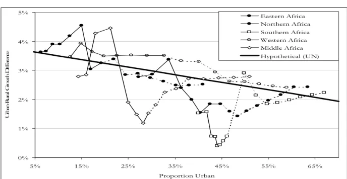
In figures 1 to 5, we plotted the trends formed by the urban-rural growth difference (rur) in the (t-5,t) time interval against the proportion urban (PU) at time t for different regions of the world. The curves read from left to right and the first point represents the year 1955. Subsequent points are defined over five-year intervals until the year 2030, the last point on the curve. The projection period is represented for each region by dotted lines from 1990.

Figure 1: Urban-Rural Growth Difference versus Proportion Urban in Africa (1950-1930, projection period represented by a dotted line)

Source: UN, 2004.

Figure 2: Urban-Rural Growth Difference versus Proportion Urban in Caribbean, South and Central America (1950-1930, projection period represented by a dotted line)

Source: UN, 2004. 0% 1% 2% 3% 4% 5% 5% 15% 25% 35% 45% 55% 65% Proportion Urban U rba n-R ur al G ro w th D if fe re nc e Eastern Africa Northern Africa Southern Africa Western Africa Middle Africa Hypothetical (UN) 0% 1% 2% 3% 4% 5% 30% 40% 50% 60% 70% 80% 90% Proportion Urban U rba n-Ru ra l G row th D if fe re nc e Caribbean Central America South America Hypothetical (UN)

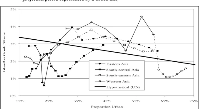
Figure 3: Urban-Rural Growth Difference versus Proportion Urban in Asia (1950-1930, projection period represented by a dotted line)

Source: UN, 2004.

Figure 4: Urban-Rural Growth Difference versus Proportion Urban in Less Developed Oceania (1950-1930, projection period represented by a dotted line)

Source: UN, 2004. 0% 1% 2% 3% 4% 5% 15% 25% 35% 45% 55% 65% 75% Proportion Urban Ur ba n-R ur al G ro w th D if fe re nc e Eastern Asia South-central Asia South-eastern Asia Western Asia Hypothetical (UN) 0% 1% 2% 3% 4% 5% 15% 25% 35% 45% 55% 65% 75% Proportion Urban U rba n-R ur al G ro w th D iffe re nc e Melanesia Micronesia Polynesia Hypothetical (UN)

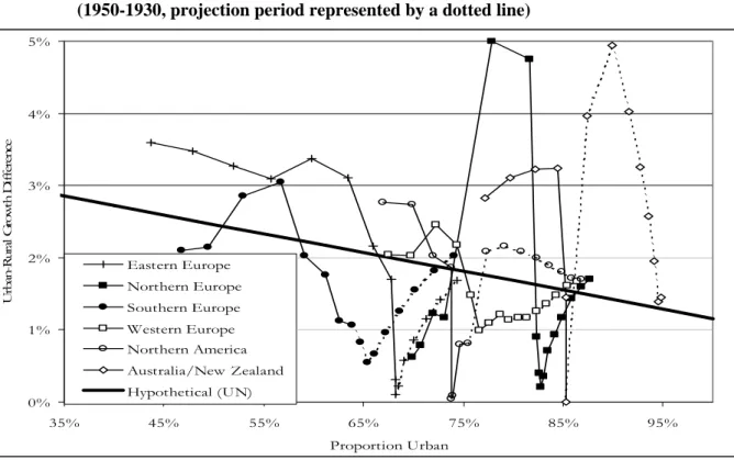
Figure 5: Urban-Rural Growth Difference versus Proportion Urban in Developed Regions (1950-1930, projection period represented by a dotted line)

Source: UN, 2004.

The reason why a linear model was used when the UN started its projection exercise in the 1980s was that at the time, very few countries had more than three observed points on the rur-PU curve from the 1950s to the 1970s. In absence of deeper historical trends, a sensible solution was to model the trend across countries at a given time. The different level of urbanisation at which these countries were captured was supposed to reflect the most likely path the less urbanised countries would follow to reach, one day, the level of the most urbanised countries.

Now that data are available from the 1950s to the 1980s, there is less reason to believe that a linear model relating rur and PU should still be fitted. In hardly any region of the world the relation follows a linear downward pattern, except maybe in Western Africa (Figure 1), South America and Central America (Figure 2). Most patterns from 1955 to 1990 follow an inverted U-curve whether in developing countries (Eastern Africa, Middle Africa, Northern Africa, Caribbean, South-Central Asia, Melanesia and Micronesia) or in developed countries (Southern Europe and Northern Europe). Other regions follow a more ambiguous pattern but almost all have seen the rur falling sharply from peak values usually attained in the 1950s and 1960s for the LDC regions, or in the 1970s and 1980s for the MDC regions. Exception to that phenomenon are found in Asia: Western Asia, which after a sharp fall in the 1970s, experienced the opposite trend in the 1980s; South-Eastern Asia experienced a rise in the 1970s and 1980s, and Eastern Asia in the 1980s, though this can be attributed to China2 _only.

Rather intriguingly, some regions, particularly in Africa but also in Oceania, show a slight increase in the rur in the 1980s that could be interpreted as a reversal of the overall downward trend. However, this upward trend is limited and rather reflects the use of the UN model of projection for some countries where data were not available prior to 1995. This shows that the method not only has an effect on the 1995-2030 projection period but also on the later part of the estimation period, i.e. in the 1980s up to 1995, as data on urbanisation were not readily available for all developing countries.

2

The peculiar case of China can be explained by the Cultural Revolution in the late 1960s to early 1970s, which forced many urbanites to live in rural areas, but also by changes in the official urban definition United Nations (2002), World Urbanization Prospects: The 2001

Revision. Data Tables and Highlights. New York: United Nations Secretariat, Population Division.

0% 1% 2% 3% 4% 5% 35% 45% 55% 65% 75% 85% 95% Proportion Urban Ur ba n-R ur al G row th D if fe re nc e Eastern Europe Northern Europe Southern Europe Western Europe Northern America Australia/New Zealand Hypothetical (UN)

1.2.

We have seen the urbanisation trends in the second half of the 20th century. Do the UN projections observe the same trends or do they depart significantly from the empirical, historical observations? The easiest way to confirm the latter is to observe the trends formed by the dotted lines on Figures 1 to 5 for the period 1990-2030. For ease of interpretation and in order to better show the effect of the UN model of projection, we added the regression result that was used to fit and to project the value of rur. Although the graphs show data grouped by world regions, whereas the UN estimation and projections were done country by country, it is clear that this method of projection has the effect of:

- Reversing the downward trend for those regions which fell below the regression line in 1995. This is particularly visible for developing Oceania and European regions (Figure 4 and 5), but also for other regions like Middle Africa (Figure 1) or South-Central Asia (Figure 3). In these regions, the rur sort of ‘bounced’ to reach the level of the regression line.

- For those regions which fell above the regression line in 1995, maintaining the rur at high level for some time before it joins the regression line.

Some other regions (South-Eastern Asia, Southern Africa, Central America and Australia-New Zealand) follow patterns that do not fit the above description, but generally, none of the trends for the projection period 1995-2030 follow the patterns of the estimation period 1950-1995, with the possible exceptions of Western Africa and Central America. The Figures make it clear that the UN projections are not prolonging historical trends. As expected—since the UN projection model applies uniformly to all countries—, all regions line up against the regression line in the vicinity of 2030.

What are the effects on the projected urbanisation level? The reversal of the downward trend and inflation of the rur have the effect of increasing urban growth in most developing countries, and maintaining urban growth at high level in more developed countries. We then expect the projected proportion urban at the 2030 horizon to be largely overestimated. In other words, the UN method of projection is implicitly imposing a unique, historically dated, MDC-oriented model of urban transition on all countries of the world, leading to a systematic overestimation of the world urbanisation.

2. IN SEARCH OF AN ALTERNATIVE MODEL FOR PROJECTING

URBANISATION

Our contention is that projections should be based on the history of urban transition and take account of the different levels of development across the world. It has been shown that there is a high correlation between the proportion urban and the level of development, measured either by gross domestic product (GDP) or by the human development index (HDI) (Davis, Henderson, 2003; Njoh, 2003). Though the causal relationship between urbanisation and development is far from clear, an endogenous projection model should apply differently depending on the specific urban history of the country at stake and should not necessarily lead to a high proportion urban for all countries or regions of the world.

However this theory—as the theory of demographic transition for that matter—, is not clear about the effect of the development characteristics on the actual level of urbanisation that each country should reach at the end of the urban transition. It is hypothesized that development as it is known in the Western world should expand to the rest of the world so that, at the end of the day, all countries should reach the same level of urbanisation, close to the level reached in the present MDC. On the contrary, the empirical evidence of the preceding section shows that the urban transition might follow different patterns according to the historical period it went through and to the level of economic development reached. In statistical terms, the curve formed by plotting rur against PU shows different shapes. Not only the modal point of the curve varies a lot (reaching a maximum of 6% in Melanesia, for example), but also the proportion urban at which the rur seems to converge to zero is different.

We will call this point of convergence the urban saturation point for convenience. It represents the point where rural and urban areas are growing at the same pace. The term saturation as employed here does not mean it is an absorbing state where the country or region is trapped after rur eventually reaches zero. In the real world of urbanisation (as shown later in this paper), cases of reverse urbanisation (when rur is less than 0) and erratic variations around a focal point (when rur is alternatively greater and smaller than 0) are not uncommon. Our concept of urban saturation is meant here to identify a theoretical point of convergence of the urban transition process that can be different from one country to another and that could possibly correspond to the urban capacity of the economy, which can itself evolve over time.

In this section, we will start by giving the principal characteristics of a model for urban projection before proposing a new model of projection based on two key principles: historical perspective and country-based approach. We will then implement the model and show that it actually fits quite well the observed urbanisation process of most countries in the world and offers a quite reasonable alternative to the UN projections.

2.1.

To follow a historical perspective on urban transition, an alternative model of projection based on macro-data should integrate two new factors: speed of urban transition and possible urban saturation, or even counter-urbanisation as seen in some countries as early as in the 1980s (Australia and New Zealand). The new models for projection should rely more on the past, empirically observed trends, and should keep the arbitrary choice to a minimum. The new projection model should be endogenous, i.e. based on the available data only, as the UN projection model is. Our objective here is not to offer a projection model with explanatory power, using a number of exogenous variables (such as GDP, HDI, etc.) that could explain the proportion urban and its trend, but to offer better projections using the known quantities only.

The model should take into account that projections do not necessarily converge toward an average behaviour. The model should allow each country or region to follow its own urban transition, leading to different level of urban saturation. A polynomial model for extrapolation should ideally conform to the inverted-U shape historically observed up to 1995 in most countries and the projected rur* will take the form:

2 , 2 , , 1 , 0 , * 5 ,t ( it) i . it i . it i F PU PU PU rur ₊ = =

β

β

β

As for the UN model, the projection will be conducted step by step, by five-year increment, the estimate for one projection period being used for the projection of the next. Before going into the details of the implementation of the polynomial model, we will demonstrate that the excess total absolute increase in urban areas should be preferred to the rur for modelling.

2.2.

The reader would have already noticed that the relation between the urban-rural growth difference (rur) and the proportion urban (PU) plays an important role in the UN projections. As noted in the UN report, the rur is a difference of rates. As such, it does not take account of the constraints imposed by the risk pool (the absolute number) in both urban and rural areas. Using intercensal rates seems perfectly sensible for interpolation because the census data represent observed boundaries and therefore the interpolation necessarily lies within the possible. For extrapolation, however, the rur, which depends largely if not mostly on migration flows, should ideally be constrained by the actual pool of the population in the origin and destination area. As mentioned earlier, the solution found by the UN is to find by way of a regression a hypothetical urban-rural growth difference for the projection period (hrur). From our empirical diagnosis this method appears inappropriate and our contention is that finding a better function for hrur will not improve the projection, as long as the rur will be used as a basis for projection. We find the projection fitting better the data at a country level when the difference of growth between urban and rural areas is measured in absolute terms rather than in relative terms. Instead of modelling the rur we will model the excess increase in urban areas, denoted xu: t t t t t t t t t t U U p R U R U U U xu _⎟⎟= − ⋅ ⎠ ⎞ ⎜⎜ ⎝ ⎛ + + ⋅ − = ₋ − − − 1 1 1 1 (1)

where

p

U

⋅

p

urban areas if the urban areas were to grow at the same rate as the total population. We chose xu because of its close relation to rur, as demonstrated in the Annex 1:

⎟⎟ ⎠ ⎞ ⎜⎜ ⎝ ⎛ + ⋅ ⋅ = − − − − 1 1 1 1 t t t t t t R U R U rur xu (2) This relation makes computation for projection easy. But the main reason for preferring xu over rur is

its ability to control for population growth. Contrary to rur, which expresses a difference between growth rates, xu depends not only on this differential but also on the total population growth. When the population grow less, the number of migrants is also diminishing, thus reducing the potential growth of the receiving area. The projection using xu will then be constrained by the overall population growth and therefore be dependent on (and sensitive to) the projection of the total population.

Instead of projecting the rur* from a polynomial regression on PU:

2 , 2 , , 1 , 0 * 5 ,t i it i it i PU PU rur ₊ =

β

β

β

2 * * t t PU PU R U rur xu = ⋅_⎜⎜⎛ ⋅ _⎟⎟⎞=

β

β

β

should converge to zero or even be negative (i.e. it should be called an excess decrease conducive to counter-urbanisation). The model is thus country-specific, historically-based and makes a minimum assumption about the form of the relation (a polynomial function) between known quantities (rur and PU).

2.3.

As they are based on National Definitions of urban areas, the UN data are subjected to variations within countries (historical variations) and between countries (geographical variations). In particular estimations for early years (1950s or 1960s) are often not consistent with the latest estimations used. In that case national trends can well be fitted using the most recent estimations. In other instances, UN estimations for the most recent periods show inconsistencies as some countries did not provide for any valuable estimation of their urban population for the last observation dates (1990, 1985 or even 1980) thus leading the UN to supplement with their own estimates. However, these estimates are based on the method of projection criticised above and can lead to biased results. To avoid any bias introduced by the UN method of projection, we will only take into consideration the UN estimations up to the time of the most recent data available at the country level, as mentioned in the UN report annex. Therefore, the estimation period will vary depending on the data availability of each country or territory3_.

Contrary to our initial belief, the polynomial model works much better than expected at the country level. Our fear was that by using a country-specific model we would end up with a lot more inconsistencies due to the varying quality of the data. If it were so, we would have to resort to a region-based model, e.g. by grouping countries in homogenous area of development. Instead, most countries follow a typical inverted U-curve as hypothesized at the beginning of this study from the urban transition theory. By fitting the excess total increase in urban areas (xu) instead of the rur, the polynomial form imposed in the model produces much better fit of historical trends that expected. The procedure to come out with the best possible fit and projection is as follows4_:

1. Fit the polynomial model on all countries for the estimation period, i.e. from 1950 to the latest date when an estimate is available on the basis of available national data—the estimation period varies from one country to another.

2. Compute the projected urban population and other necessary indicators for the next five-year interval.

3. Compute the same for the next five-year interval using previous projections up to 2030, excluding countries that reach 100% urban by projection.

4. Identify the outliers, i.e. the countries for which the parameter

β

5. Examine the pattern of urban growth for the identified outliers and identify the possible country-specific (historical) outliers in the estimation of urban population. This is done easily by identifying the early periods’ estimations (generally in the 1950s and 1960s) that influence most the unexpected fit, although some bad fit can also be caused by recent estimation (e.g. for the 1990s or even the 1980s). The earlier estimates, e.g. for the 1950s or the 1960s, are retained for computation even if they are not based on national data, so long as the country is not an outlier. 6. Fit the polynomial model on all countries for the estimation period, after excluding some

observation points for the countries identified as outliers.

7. Do again step 1 to 6 until all possibilities of exclusion of country-specific observations are explored.

3

In this paper, and for ease of presentation, the term ‘country’ includes territories (very often islands) that are not necessarily politically independent but for which the UN gathered specific data on urbanisation. The word country in this paper implies no judgment about the legal or other status of a territory.

4

Computations were made using the Stata 8.0 program xtreg with random effect (re option) and the country as the group variable (i(country) option). Specific models were run on Nigeria and Aruba. For all other countries, the final model R2 _{(measuring the}

percentage of the variance explained) is 83.45% and the Wald Chi2 _{with 632 degree of liberty is 28349.48 (significant at the 1 per 10,000}

Countries where all the population is urban are excluded from the projection exercise: Hong Kong, Macao, Singapore, Gibraltar, Holy See (Vatican), Monaco, Anguilla, Cayman Islands, Bermuda, Nauru. These countries are all set on small territories or islands, with no possibility of extension, so that their urbanisation has reached an absorbing state, i.e. these countries are not supposed to gain rural population at a later stage. Only three small countries or territories, all situated in Polynesia, were 0% urban: Pitcaim (population<100 inhabitants), Tokelau (<1500), Wallis and Futuna Islands (<14500). Whether these few countries which did not so far gain any urban population should one day have an urban population is debatable but no model can be fit for those tiny countries.

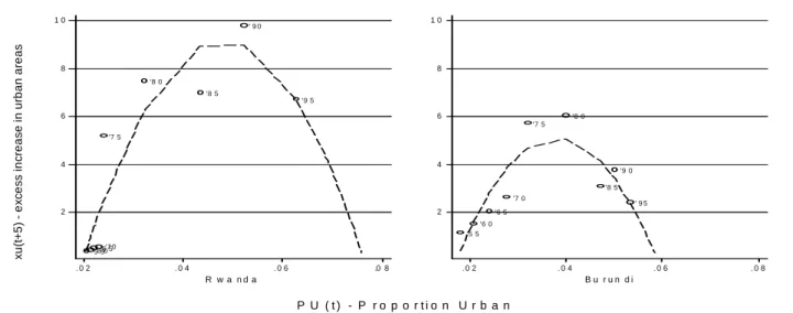
The Figure 6 shows for two countries, Rwanda and Burundi, how the polynomial curve is fitted on the historical trend from 1950 to 1990 (xu at t versus PU at t-5). The Figure 7 shows how the fit translates in terms of rur and PU as well as the projected trend up to 2030. Note that both countries converge toward a saturation of the proportion urban in 2030 (<6% for Rwanda, <8% for Burundi). However, these projections do not take account of the effect of the 1994 genocide in Rwanda and of the subsequent wars, which effect on urbanisation remains to be seen.

Figure 6: Excess Increase in Urban Areas Estimates (xut+5) and Polynomial Model Fit (xu* t+5)

versus Proportion Urban (PUt) for Rwanda and Burundi

Figure 7: Urban-Rural Growth Difference Estimates (rurt) and Polynomial Model Fit (rur*t)

versus Proportion Urban for Rwanda and Burundi '5 5'6 0'6 5'7 0 '7 5 '8 0 '8 5 ' 9 0 '9 5 2 4 6 8 1 0 . 0 2 . 0 4 . 0 6 .0 8 R w a n d a '5 5 '6 0 '6 5 '7 0 '7 5 '8 0 '8 5 '9 0 ' 9 5 2 4 6 8 1 0 . 0 2 . 0 4 . 0 6 . 0 8 B u r u n d i x u (t + 5 ) ex c e s s inc reas e in ur ba n ar ea s P U ( t ) - P r o p o r t i o n U r b a n '7 5 '80 '8 5 '9 0 .0 4 .0 6 .0 8 ' 75 '8 0 .0 4 .0 6 .0 8 al G rowt h Dif fer en c e

2.4.

The Annex 2 shows the importance of outliers identified after running the polynomial model. In this Annex, the great outlying countries, for which we had to find specific solutions, are indicated. Other outliers were more easily dealt with and are also listed in the Annex 2 along with the solution found to integrate them in the general model. We were not able to find any adjusting solution for only one small Caribbean island, Barbados (less than 270,000 inhabitants in 2000). For this country, we simply replicated the level of urbanisation attained in 1990, the year of the latest estimate, as the proportion urban did not vary much before.

Two cases are worth mentioning here. We had to run a specific model for Nigeria. In this country, hardly any data is available, except two unreliable censuses (1963 and 1991), to support any valuable projection on urbanisation. The projection using the standard polynomial model on xu proved unrealistic (leading to exponential urban growth from 2010: the proportion urban would reach about 80% in 2030 and still increase after), because the overall population growth is probably overestimated for the country. Using rur proved more realistic, but the projections thus obtained should not be taken as very reliable either and are reported in the tables for the sake of offering a reasonable estimate for West Africa and for Africa as a whole. Another exception is Aruba Island in the Caribbean for which we run a simple regression model of xu on PU, without the PU2 component. Again, the projection should not be considered as very reliable for this country.

Other special corrections include correcting the population urban in Kenya and in Senegal. In Kenya, the proportion urban was grossly overestimated to 34.8% in the 1999 Census report and does not reflect the existing core urban population but the local authorities instead, i.e. with no consideration of the size of the towns and of their limits. This undocumented change of definition led the UN to increase the estimates of the level of urbanisation at earlier dates (1995, 1990 and even 1985). Our correction for Kenya consisted in estimating the level of urbanisation in 1990 as per the published 1989 Census results and in discarding the UN estimates for 1995 and 2000. For Senegal, we used the latest 2002 Census results (not considered in the UN report) to estimate the level of urbanisation in 1990, 1995 and 2000, as the previous census was done in 1987.

A last special case is with Colombia. In this country, the estimates for 1980 and 1985 looked inconsistent with the historical trend before 1980 and after 1985. We simply deleted those two observation points and found projections more compatible with the estimates for the years 1990 to 2000.

We had to adjust the model for 64 (i.e. 28%) out of 228 countries or territories of the UN database. The adjusted countries represent 43.2% of the world population en 2000 and China alone 21.0%. The adjustments were important in Southern Africa (affecting the estimates for 94% of the population of this region), Eastern Asia (86%, representing China only), South Eastern Asia (77%), Western Africa (73%), Western Asia (62%), Western Europe (54%), Eastern Africa (36%) and Micronesia (32%). Two third of the adjustments (representing 30.8% of the world population) involved the removal of some early estimation of urbanisation, mostly the 1950s and 1960s estimates, i.e. applying the polynomial model on the most recent data. These corrections originate in poor quality of data or in changes of definition of urban areas. The adjustments consisted for the remaining one third of correction cases (representing 12.4% of the world population) in removing the latest estimations that appeared inconsistent with historical trends. This is where the adjustments are the most debatable. We would of course prefer to use recent estimates as they are supposed to reflect better the current level of urbanisation. However the latest estimates are subjected to definitional changes as much as the earliest estimates. Kenya is a good example where a change of definition led to an unexpectedly high growth in urban areas. Because the author happens to live in Kenya, he was able to identify the definitional problem and make the necessary corrections. But certainly similar problems may arise for other countries identified as outliers, though it is not in the capacity of the author to document them all. For ease of interpretation of the results, the Annex 2 is offering a correction score attached to the estimates depending on the extent of the corrections made on each outlier (score 1 for mild correction to score 5 for severe correction). A detailed examination of the countries identified as outliers is needed to produce better projection estimates in the future.

Despite a number of outliers, and after some adjustment, the polynomial model fits quite well 89.5% of all countries, representing 87.6% of the world population, if we include in those figures the countries with minor corrections (for which only the early estimates, from 1950 but no later than 1975, were removed), i.e. excluding the serious outliers with a correction score greater than 2 (see Annex 2). Despite the variety of the definition of urban areas across countries and its occasional change over time in some countries, the results are certainly confirming the overall validity of the urban transition model for the estimation period.

3. A COMPARISON OF THE RESULTS OBTAINED THROUGH THE UN AND

THE POLYNOMIAL MODELS OF PROJECTION

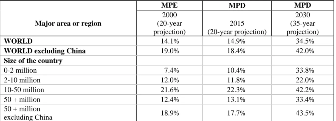
To confirm the validity of the model for the projection period, one needs to wait until estimates are produced for the year 2000 and more on the basis of country data. However it is possible to anticipate on the validity of the model by comparing the discrepancy between UN projections and country data for earlier projection periods with the discrepancy between projections using the UN model and the polynomial model. If the UN model is systematically overestimating the urban population and if the polynomial model better fits the historical trend, then the discrepancy observed should be comparable. For the first type of discrepancy, we rely on the estimate of the Mean Percentage Error (MPE) computed by Barney Cohen (2004) by comparison of the projection made in the 1980 UN report with the estimates for 2000 made in the 2001 UN report. We measured the second type of discrepancy using the Mean Percentage Difference by comparison of the projections obtained by the UN model and by the polynomial regression model. The Table 1 contains the detailed MPD by region of the world while the Table 2 compares the MPE and the MPD by country size for the 20-year projection period. We chose a long projection period for comparison because the MPE that B. Cohen computed might be more conservative for shorter projection period. To compute the MPE, B. Cohen used the 2000 estimates from the 2001 UN report, nicknamed “‘actual’ data” in his paper, which are not totally based on country data since not all countries had data available for this date. Even in the 2003 UN report, only the 1995 data are considered to be mostly based on country data whereas the 2000 estimates are a mix of estimates and projections. Therefore for our own computation of MPD, we considered the UN projections to start from 1995: the 20-year projection is for 2015 and the 35 year projection is for 2030. The 20-year projection period seems more reasonable to compare MPD and MPE as the bias in measuring MPE will be minored by the difference due to the UN projection method.

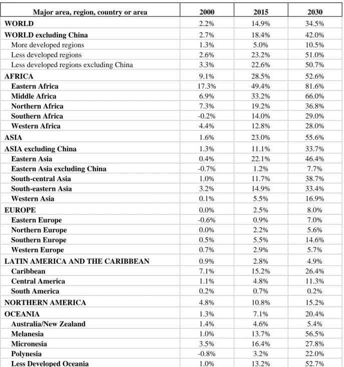
If the polynomial model better fits the historical trend than the UN model, then the MPE and MPD should have comparable values, though the projections started from lower level of urbanisation in the case of MPE. The distribution of MPE and MPD are indeed strikingly similar for the 20-year projection period. The overestimation of the urban population by the UN over the 1980-2000 period seems to replicate almost identically for the 1995-2015 period, for all country size, and looks worse when we exclude China (Table 2). As observed by B. Cohen on a different regional break-down, the discrepancy is more important for developing countries (Table 1). The difference between the UN model and the polynomial model is very high for the whole of Africa and for Eastern Africa and Middle Africa in particular. The difference is also substantial in Eastern Asia mainly because of China, in South-Central Asia and South-Eastern Asia, as well as in the Caribbean, Melanesia and Micronesia. All those regions are significantly less developed that others, but the difference is also

Table 1: Bias of UN projections as measured by the Mean Percentage Difference in Urban Population Projections

Major area, region, country or area 2000 2015 2030 WORLD 2.2% 14.9% 34.5%

WORLD excluding China 2.7% 18.4% 42.0%

More developed regions 1.3% 5.0% 10.5%

Less developed regions 2.6% 23.2% 51.0%

Less developed regions excluding China 3.3% 22.6% 50.7%

AFRICA 9.1% 28.5% 52.6% Eastern Africa 17.3% 49.4% 81.6% Middle Africa 6.9% 33.2% 66.0% Northern Africa 7.3% 19.2% 36.8% Southern Africa -0.2% 14.0% 29.0% Western Africa 4.4% 12.8% 28.0% ASIA 1.6% 23.0% 55.6%

ASIA excluding China 1.3% 11.1% 33.7%

Eastern Asia 0.4% 22.1% 46.4%

Eastern Asia excluding China -0.7% 1.2% 7.7%

South-central Asia 1.0% 11.7% 38.7% South-eastern Asia 3.2% 14.9% 33.4% Western Asia 0.1% 5.5% 16.9% EUROPE 0.0% 2.5% 8.0% Eastern Europe -0.6% 0.9% 7.0% Northern Europe 0.0% 2.2% 5.6% Southern Europe 0.5% 5.5% 14.6% Western Europe 0.7% 2.9% 5.7%

LATIN AMERICA AND THE CARIBBEAN 0.9% 2.8% 4.9%

Caribbean 7.1% 15.2% 26.4% Central America 1.1% 4.8% 11.3% South America 0.2% 0.7% 0.2% NORTHERN AMERICA 4.8% 10.8% 15.2% OCEANIA 1.3% 7.1% 20.4% Australia/New Zealand 1.4% 4.6% 5.4% Melanesia 1.0% 13.7% 56.5% Micronesia 3.5% 16.4% 27.8% Polynesia -0.8% 3.2% 22.0%

Less Developed Oceania 1.0% 13.2% 52.7%

Source: our own computation by comparison of the UN projections and the polynomial regression model. MPD is weighted by projected

Table 2: Bias of UN projections as measured by the Mean Percentage Error and the Mean Percentage Difference in Urban Population Projections

MPE MPD MPD Major area or region

2000 (20-year projection) 2015 (20-year projection) 2030 (35-year projection) WORLD 14.1% 14.9% 34.5%

WORLD excluding China 19.0% 18.4% 42.0%

Size of the country

0-2 million 7.4% 10.4% 33.8% 2-10 million 12.0% 11.8% 22.0% 10-50 million 21.6% 22.3% 42.2% 50 + million 12.4% 13.1% 33.4% 50 + million excluding China 18.9% 17.7% 43.5%

Source: MPE: Table 4, Cohen (2004). 10 years: comparison of projection in 1980 UN report with estimates for 2000 as per 2001 UN report.

20 years: comparison of projection in 1991 UN report with estimates for 2000 as per 2001 UN report.

Source MPD: our own computation by comparison of the projections obtained by the UN model and by the polynomial regression model.

MPE is weighted by population size in 2000 whereas MPD is weighted by projected population size.

Table 3 gives summary measures of urbanisation at the 2030 horizon using the UN and the polynomial model. The proportion urban would be 49.2% in the latter against 60.8% in the former, a difference of 11.6 percentage points. In absolute term, the difference in the projected urban population is 947 million. Developing countries account for 90.3% of this difference, Asia alone for 69.9% and Africa for 19.2% (Table 3). Some Asian countries particularly contribute to the difference between the two estimations (detailed results not shown here): China (31.7%), India (22.4%), as well as other countries of the Indian sub-continent like Bangladesh (3.8%) and Pakistan (3.0%), and also Indonesia (3.1%). Among developed countries, United States of America are the main contributor to the difference in the world estimation (4.5%).

Obviously any projection will be sensitive to the estimation in these countries, which are also among the most populous in the world. Because they concentrate a large share of the world population, China (1.28 billion inhabitants in 2000, 1.45 in 2030) and India (1.02 billion in 2000, 1.42 in 2030) are of particular concern regarding urbanization. In the case of China, the Cultural Revolution led to a sharp slow-down in the late 1960s followed by a sharp rise in the urban growth in the late 1970s. However our projections predict that the urban growth should start to decline at the end of the 20th century and that the proportion urban in China should stabilize at less than 40% from 2030. This departs largely from the UN projections predicting figures of 35.8% in 2000 and 60.5% in 2030. In our projection, the stabilization of the proportion urban at what would seem low level is partly due to the definition of urban areas. China is using a very high threshold (100,000 inhabitants) together with a functionalist definition of smaller urban agglomeration (majority of non-agriculture activities). Using a more standard definition of urban areas (e.g. agglomerations of 10,000 inhabitants or more) would obviously lead to a much higher level of urbanization. One has to bear in mind that all projections are made according to the definition used in each country. The projections are then not strictly comparable for all countries. Note that part of the overestimation by the UN projections originates in applying a regression model on urbanization data that are not based on a standard definition of urban areas. By so

Table 3: Comparison of UN model (model A) and polynomial model (model B) for urbanisation projections at the 2030 horizon

Proportion Urban Urban-Rural Growth Difference (2025-2030) Major area (A) (B) (B) – (A) Relative difference in Urban population Difference in Urban population (absolute) Difference in Urban population (%) (A) (B) World 60.8% 49.2% -11.6% -19.1% -946,841 100.0% 2.08% 0.13% More developed regions 81.7% 74.3% -7.4% -9.1% -92,123 9.7% 1.93% 0.16% Less developed regions 57.1% 44.6% -12.4% -21.7% -854,718 90.3% 2.32% 0.29% AFRICA 53.5% 40.5% -13.0% -24.3% -181,432 19.2% 2.31% 0.45% Eastern Africa 41.0% 27.2% -13.7% -33.5% -63,456 6.7% 2.52% 0.85% Middle Africa 54.4% 34.1% -20.3% -37.4% -38,860 4.1% 2.80% -0.02% Northern Africa 63.4% 50.5% -12.8% -20.2% -34,272 3.6% 2.43% 0.33% Southern Africa 67.0% 52.3% -14.7% -21.9% -7,149 0.8% 2.23% 0.09% West Africa 58.9% 50.1% -8.8% -14.9% -37,695 4.0% 2.41% 0.83% ASIA 54.5% 41.0% -13.5% -24.9% -662,080 69.9% 2.49% 0.20% Eastern Asia 62.6% 44.0% -18.7% -29.8% -309,725 32.7% 2.58% 0.00% South-central Asia 43.7% 32.8% -11.0% -25.1% -240,483 25.4% 2.93% 0.35% South-eastern Asia 60.7% 48.5% -12.2% -20.2% -87,108 9.2% 2.56% 0.54% Western Asia 72.3% 64.7% -7.7% -10.6% -24,764 2.6% 1.58% -0.17% EUROPE 79.6% 74.3% -5.3% -6.6% -36,182 3.8% 1.84% 0.21% Eastern Europe 74.3% 69.6% -4.7% -6.3% -12,145 1.3% 1.69% 0.01% Northern Europe 87.7% 83.5% -4.3% -4.9% -4,260 0.4% 1.71% 0.11% Southern Europe 74.1% 65.4% -8.7% -11.7% -12,026 1.3% 2.03% 0.01% Western Europe 86.4% 82.3% -4.1% -4.7% -7,752 0.8% 1.68% 0.43%

LATIN AMERICA &

CARIBBEAN 84.6% 82.1% -2.5% -3.0% -17,976 1.9% 1.67% 1.08% Caribbean 73.3% 60.4% -12.9% -17.6% -5,857 0.6% 1.87% -0.06% Central America 77.5% 70.9% -6.6% -8.5% -12,730 1.3% 1.82% 0.21% South America 88.6% 88.8% 0.1% 0.1% 611 -0.1% 1.60% 2.13% NORTHERN AMERICA 86.9% 75.4% -11.4% -13.2% -46,611 4.9% 1.70% -0.01% OCEANIA 74.9% 68.7% -6.2% -8.2% -2,560 0.3% 0.48% -0.50% Australia/New Zealand 94.9% 90.0% -4.9% -5.1% -1,375 0.1% 1.45% 0.35% Melanesia 27.2% 18.2% -9.0% -33.2% -1,046 0.1% 2.65% -0.24% Micronesia 81.2% 70.0% -11.2% -13.8% -84 0.0% 1.85% 0.09% Polynesia 55.0% 48.4% -6.5% -11.9% -55 0.0% 2.36% 0.34% Less Developed Oceania 32.0% 23.0% -9.0% -28.1% -1,184 0.1% 2.27% -0.18%

We don’t expect the same definitional problem with India because this country uses a much lower threshold (5,000 inhabitants), together with a functionalist approach (administrative centers, non-agricultural activities…). According to our projections, the level of urbanization in India would stabilize slightly above 31% from 2030. This compares with 41.4% in the UN projection for 2030 but with persistent growth after this date. Here the difference in estimation is mainly attributed to the difference in modeling.

If the polynomial model proved right, the majority of the developing world would not live in urban areas by 2030. The population would stay predominantly rural in Africa and in Asia (Table 3). Even more importantly, the potential for future urban growth is very much reduced in the projections based on the polynomial model. To measure this potential, we used the urban-rural growth difference (rur) for the period 2025-2030 (Table 3). In the UN projections the rur ranges in each region between 1.5% and 3% whereas in the polynomial projections the rur hovers around 0% and exceeds 2% only in South America, while it is sometimes negative (as in Western Asia and Melanesia), indicating reverse urbanisation.

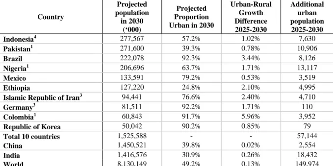
The UN methodology used for projection inevitably forecasts that the proportion urban would one day reach 100%. On the contrary, the polynomial model indicates that urban saturation could be attained not long after 2030. Therefore, there is a huge discrepancy between the UN projections and our projections based on the historical patterns of urban transition. According to the polynomial model, very few countries would still have in 2030 a high potential for urban growth. The Table 4 indicates the most populous countries (with 50 million inhabitants or more in 2030) which would still have a high rur (more than 0.5% a year in the 2025-2030 period). Quality of the projections notwithstanding (6 of them were subjected to special corrections before projections, see Annex 2), those large, mostly developing countries5 _{representing 18.8% of the world population in 2030 would account for 38.1% of}

the urban population increase between 2025 and 2030. India with a rur of only 0.26% a year would account for 12.3% of the world urban population increase. To summarize, 10 developing countries would contribute to more than half of the world urban population increase in the 2025-2030 period. Many of the remaining countries would have reached their urban saturation level, contributing marginally to the world urban growth after 2030.

Table 4: Ten largest countries (>50 million) still having a high urban growth potential (>0.5%) in the 2025-2030 period according to the projection using the polynomial model Country Projected population in 2030 (‘000) Projected Proportion Urban in 2030 Urban-Rural Growth Difference 2025-2030 Additional urban population 2025-2030 Indonesia4 277,567 57.2% 1.02% 7,630 Pakistan1 271,600 39.3% 0.78% 10,906 Brazil 222,078 92.3% 3.44% 8,126 Nigeria1 206,696 63.7% 1.71% 13,117 Mexico 133,591 79.2% 0.53% 3,519 Ethiopia 127,220 24.8% 2.10% 4,995

Islamic Republic of Iran3 94,441 76.6% 2.40% 4,710

Germany3 81,511 92.2% 1.71% 110 Colombia1 60,843 91.7% 5.96% 3,952 Republic of Korea 50,042 90.2% 0.85% 79 Total 10 countries 1,525,588 - - 57,144 China 1,450,521 39.8% 0.02% 2,554 India 1,416,576 30.9% 0.26% 18,432 World 8,130,149 49.2% 0.13% 149,974

Note: Countries subjected to corrections in the polynomial model are indicated by their correction score: 1 (mild correction),

3 (high correction), 4 (very high correction). The estimates for those countries are therefore to be cautiously interpreted.

CONCLUSION: Improving projection models

It is clear from our analysis that the UN projections are biased and lead to a gross overestimation of urbanization trends. Contrary to the common belief, the UN projections are not based on the extrapolation of historical trends. We proved that this can be attributed mainly to an inappropriate projection model that systematically biases the urban estimates upward, and also to the quality of the

To start with, our polynomial model has limitations that should be taken into account to refine the projections:

- Our projections are based on the World Urbanization Prospects published by the UN, with estimates of the urban and total population by 5-year intervals from 1950. In reality, censuses are not always available from that date and are rarely conducted every five years and our model is therefore partly based on interpolations. The original UN data set is not made available to the public but it would be better to use (and not more difficult to implement) the original estimation points from census data or other sources.

- Our projections show that the information on urbanisation is better used at a country level than at a sub-regional level or continental level. An improvement would be to work at a sub-country level for such countries as China, India, etc.; where there are huge discrepancies between provinces or States.

- More effort should be devoted at finding better estimations for the countries for which we had to make specific corrections. In these countries the problem is more with the data that form the base for projection than with the model itself.

- International comparisons become difficult when countries are using very different definitions. A particular effort should be directed at evaluating the population in urban areas according to an internationally recognised definition. An alternative to the projection of the overall urban population would be the projection of the urban population above high thresholds (e.g. agglomerations of more than 20,000, 50,000, 100,000 or 500,000 inhabitants) that could easily be computed using a list of towns and cities ranked by size in each country. A regression model based on the estimates obtained at each threshold could then be used to evaluate the urbanisation rate with a standard threshold at a lower level (e.g. 10,000 inhabitants).

Whatever the alternative model, the expected results if they are based on historical trends will change the perception that we have of urbanisation and of its relation to development. The urban population could be as much as 1 billion less than expected and the LDC might not, after all, become predominantly urban. From our projections, it would appear that in a foreseeable future the level of urbanisation will most probably be much more heterogeneous than previously thought. Whether this is good or bad news depends on the perspective than one has on development. If the correlation between on one hand urbanisation and on the other hand GDP, HDI, poverty index or other social and economic development indicators is confirmed, then the tentative urban projections presented here reflect the persistence of poverty and of great economic inequalities over the world. Our projections also call for the revision of the projection of the global population as the reduction of mortality and fertility (the speed of the demographic transition is often attributed to the influence of the urban way of life) might not be so important. The projections of urban population have great consequences on environmental policies. In al less urbanised world, the developed countries would still be responsible for most of the greenhouse gas emission while most of the natural resources would remain in the developed world.

BIBLIOGRAPHY

Balk, D., Pozzi, F., Yetman, G., Nelson, A., Deichmann, U. (2004), « Methodologies to Improve Global Population Estimates in Urban and Rural Areas », Boston MA, USA: Population Association of America, 6.

Bocquier, P., Madise, N. J., Zulu, E. (2005), « Mesurer Rétrospectivement La Mortalité En Afrique, En Situation De Forte Migration Des Vivants, Des Malades… Et Des Morts », Population. Cohen, B. (2004), « Urban Growth in Developing Countries: A Review of Current Trends and a

Caution Regarding Existing Forecasts », World Development,Vol. 32, n°1, pp. 23-51.

Davis, J. C., Henderson, J. V. (2003), « Evidence on the Political Economy of the Urbanization Process », Journal of Urban Economics,Vol. 53, pp. 98-125.

EIA (2004), International Energy Outlook. Washington, D.C.: Energy Information Administration, 256p.

Hugo, G., Champion, A. (2003), New Forms of Urbanisation. Aldershot: Ashgate IEA (2004), World Energy Outlook. Paris, France: International Energy Agency, 550p. Moriconi-Ebrard, F. (1993), L'urbanisation Du Monde. Paris: Anthropos, 372p.

Moriconi-Ebrard, F. (1994), Geopolis - Pour Comparer Les Villes Du Monde. Paris: Anthropos, 246p. National Research Council (2003), Cities Transformed - Demographic Change and Its Implications in

the Developing World. Washington D.C.: The National Academies Press, 529p.

Njoh, A. J. (2003), « Urbanization and Development in Sub-Saharan Africa », Cities,Vol. 20, n°3, pp. 167-174.

UNDP, UNEP, World Bank, World Resources Institute (2003), World Resources 2002-2004: Decisions for the Earth: Balance, Voice, and Power. Washington, D.C.: United Nations Development Programme, United Nations Environment Programme, World Bank, World Resources Institute, 328p.

UN-Habitat (2003), Slums of the World: The Face of Urban Poverty in the New Millenium? Monitoring the Millenium Development Goal, Target 11 - World-Wide Slum: Dweller Estimation. Nairobi: UN-Habitat

United Nations (1997), World Urbanization Prospects: The 1996 Revision. New York: United Nations Secretariat, Population Division

United Nations (2002), World Urbanization Prospects: The 2001 Revision. Data Tables and Highlights. New York: United Nations Secretariat, Population Division

World Bank (2003), Global Economic Prospects and the Developing Countries 2004. Washington, D.C.: World Bank, 334p.

Zelinsky, W. (1983), « The Impasse in Migration Theory: A Sketch Map for Potential Escapees », in Population Movements : Their Forms and Functions in Urbanization and Development, ed. par P. A. Morrison. Liège: Ordina - IUSSP, pp. 19-46.