UNIVERSITÉ DU QUÉBEC À MONTRÉAL
ÉVALUATION DES NUAGES ET DE LEUR INTERACTION AVEC LE
RAYONNEMENT DANS LE MODÈLE GEM
MÉMOIRE
PRÉSENTÉ
COMME EXIGENCE PARTIELLE
DE LA MAÎTRISE EN SCIENCES DE L'ATMOSPHÈRE
PAR
DANAHÉ PAQUIN-RICARD
UNIVERSITÉ DU QUÉBEC
À
MONTRÉAL Service des bibliothèquesAvertissement
La diffusion de ce mémoire se fait dans le respect des droits de son auteur, qui a signé le formulaire Autorisation de reproduire et de diffuser un travail de recherche de cycles supérieurs (SDU-522 - Rév.01-2006). Cette autorisation stipule que «conformément
à
l'article 11 du Règlement no 8 des études de cycles supérieurs, [l'auteur] concèdeà
l'Université du Québecà
Montréal une licence non exclusive d'utilisation et de publication de la totalité ou d'une partie importante de [son] travail de recherche pour des fins pédagogiques et non commerciales. Plus précisément, [l'auteur] autorise l'Université du Québecà
Montréalà
reproduire, diffuser, prêter, distribuer ou vendre des copies de [son] travail de rechercheà
des fins non commerciales sur quelque support que ce soit, y compris l'Internet. Cette licence et cette autorisation n'entraînent pas une renonciation de [la] part [de l'auteur]à
[ses] droits moraux nià
[ses] droits de propriété intellectuelle. Sauf entente contraire, [l'auteur] conserve la liberté de diffuser et de commercialiser ou non ce travail dont [il] possède un exemplaire.»REMERCIEMENTS
Je tiens à remercier mes directeur et co-directeur, Colin Jones et Paul Vaillancourt, pour leur soutien et leur aide tout au long de ma maîtrise et plus particulièrement mon directeur pour ses bons conseils, sa patience et ses encouragements lors de la rédaction de l'article. Je tiens aussi à remercier mes collègues de bureau qui, à tous les jours, rendent l'environnement de travail stimulant et qui sont toujours disponibles pour offrir leur aide ét leur soutien moral. Finalement, je remercie mon copain pour toute sa patience, son soutien et son enthousiasme envers mes projets de recherche.
TABLE DES MATIÈRES
LISTE DES FIGURES . Vll
LISTE DES TABLEAUX Xl
LISTE DES ABRÉVIATIONS, SIGLES ET ACRONYMES xiii
CHAPITRE l RÉSUMÉ . . . xv INTRODUCTION 1 ARTICLE 7 ABSTRACT . 9 1.1 Introduction. 10 1.2 Methodology 13
1.2.1 Model description and integration 13
1.2.2 Evaluated variables . 14
1.2.3 Observation datasets .
16
1.3 Results . 20
1. 3.1 Large-scale meteorology 20
1.3.2 All-sky surface radiation fluxes 22
1.3.3 Cloud fraction .
26
1.3.4 Surface radiation fluxes for clear-sky conditions.
29
1.3.5 Surface radiation fluxes for overcast conditions 33
1.4 Conclusions and Discussion 45
LISTE DES FIGURES
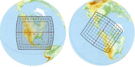
l.1 The two simulation domains centered over the ARM-SGP site (left) and the ARM-NSA site (right). Only every 5 grid points (left) or 10 grid points (right) of the original grids are shown while the dashed lines in dicate nesting and sponge zones where the model is gradually forced to follow the LBCs. The observation sites are marked with a red cross. 15 1.2 Mean diurnal cycle of different CF observations for (a) SGP summer and
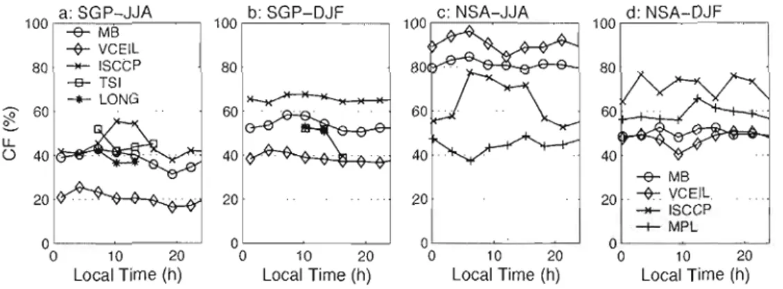
(b) win ter for 2000-03, (c) NSA summer and (d) win ter for 2004. . . .. 17 1.3 Three-day mean surface pressure (P) and IWV at SGP for (a) summer
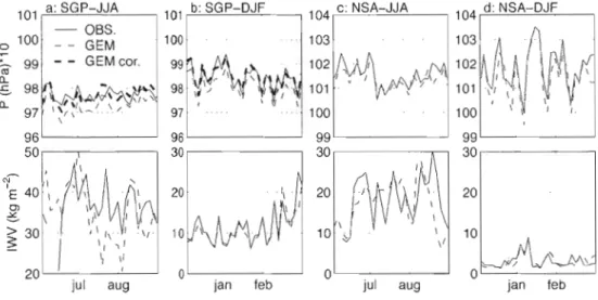
2000, (b) winter 2000/01, and NSA for (c) summer 2004 and (d) winter 2004/05. For SGP, the thick dashed \ine represents a correction of 4.47 hPa applied to the modeled surface pressure to account for the 38 f i
difference in altitude between observations and mode!. . . . 21
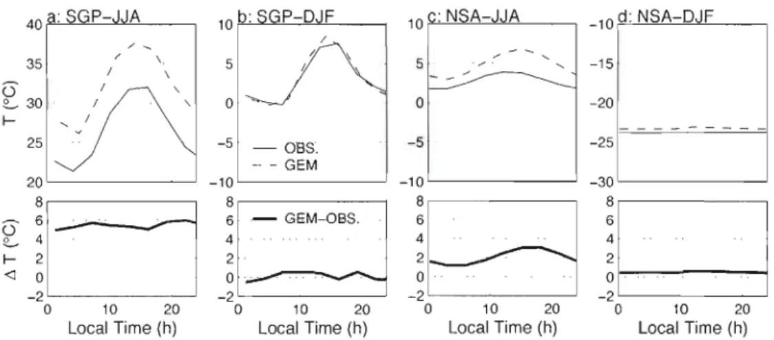
1.4 Tvlean diurnal cycle of three-hourly mean 2 m temperature for (a) SGP JJA, (b) SGP-DJF, (c) NSA-JJA and (d) NSA-DJF. The bottom row
shows corresponding bias. 22
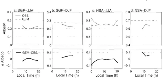
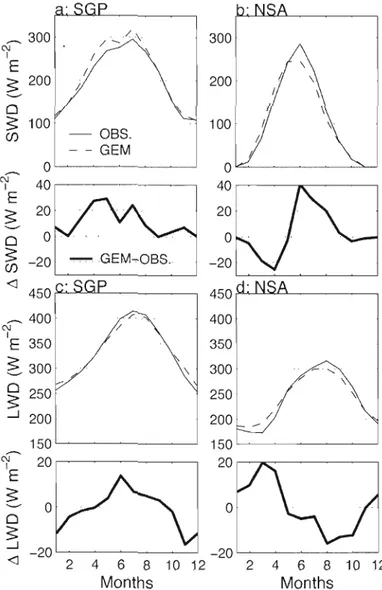
1.5 Mean diurnal cycle of three-hourly mean surface a[bedo for (a) SGP-JJA, (b) SGP-DJF, (c) NSA-J,JA ancl (cl) NSA-DJF. The bottom row shows corresponding bias. . . 23 1.6 Mean annual cycle of monthly mean (a-b) SWD and (c-d) LWD at the
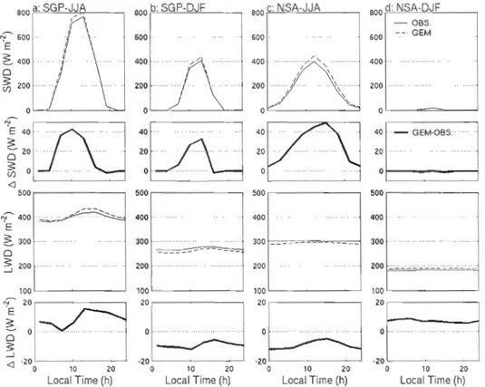
surface for (a/c) SGP and (b/d) NSA with corresponding bias. . . . 24 1.7 Mean diurnal cycle of SWD and LWD at the surface for (a) SGP-JJA,
Vlll
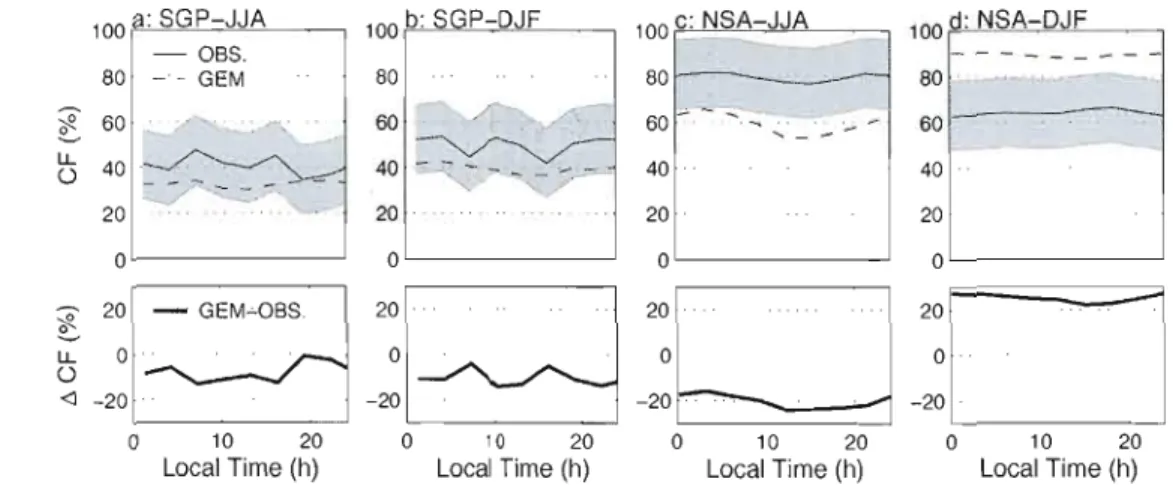
1.8 Mean diurnal cycle of CF for (a) SGP-JJA, (b) SGP-DJF, (c) NSA-JJA and (d) NSA-DJF. The light shaded zone around the observed curve represents a degree of uncertainty regarding the absolute accuracy of the plotted observed CF (± 15 %). The bottom row shows corresponding bias. 27
1.9 Frequency of occurrence of 3-hourly mean CF for (a) SGP-JJA, (b) SGP DJF, (c) NSA-JJA and (d) NSA-DJF. . . . .. 28
1.10 Mean diurnal cycle of SWD and LWD at the surface for clear-sky con ditions for (a) SGP-JJA, (b) SGP~DJF, (c) NSA-JJA and (d) NSA-DJF with corresponding bias. . . . .. 30
1.11 Mean diurnal cycle of IWV for (a) SGP-JJA, (b) SGP-DJF, (c) NSA-JJA and (d) NSA-DJF. The bottom row shows corresponding bias. . . . 31
1.12 SWD as a function of IWV for clear-sky for (a) SGP-JJA, (b) SGP-DJF and (c) NSA-JJA. Median is plotted for model and observations. Shown are only values for SZA below 65°. . . . .. 33
1.13 LWD as a function of IWV for clear-sky for (a) SGP-JJA, (b) SGP DJF, (c) NSA-JJA and (d) NSA-DJF. Median is plotted for model and observations. The inset only represents a zoom over the results for NSA DJF. . . .. 34
1.14 Mean diurnal cycle of SWD and LWD at the surface for 0:rercast condi tions for (a) SGP-JJA, (b) SGP-DJF, (c) NSA-JJA and (d) NSA-DJF with corresponding bias. . . . .. 35
1.15 Mean diurnal cycle of LWP for (a) SGP-JJA, (b) SGP-DJF, (c) NSA-JJA and (d) NSA-DJF. The bottom row shows corresponding bias. . . . 37
1.16 Frequency of occurrence of 3-hourly mean LWP and CWP (liquid+ice) for (a) SGP-JJA, (b) SGP-DJF, (c) NSA-JJA and (d) NSA-DJF. . . .. 38
IX
1.17 Frequency of occurence of 3-hourly mean LWP for different thresholds of precipitation for (a) SGP-JJA, (b) SGP-DJF, (c) NSA-JJA and (d)
NSA-DJF. 40
1.18 F'requency of occurence of 3-hourly accumulated precipitation for (a) SGP-JJA, (b) SGP-DJF, (c) N8A-JJA and (d) NSA-DJF. First bins from model and observations are divided by 10. . . .. 42 1.19 SWD as a function of LWP for overcast conditions for (a) SGP-JJA, (b)
SGP-DJF and (c) NSA-JJA. Median is plotted for model and observa tions. The figure at the bot tom right represents a zoom over the black box for SGP-JJA. Shown are only values for SZA below 85°. 43 1.20 Mean diurnal cycle of SWD for NSA-JJA with and without precipitation. 44 1.21 LWD as a function of LWP for overcast conditions for (a) SGP-JJA, (b)
SGP-DJF, (c) NSA-JJA and (d) NSA-DJF. Median is plotted for model and observations. . . .
46
LISTE DES TABLEAUX
LISTE DES ABRÉVIATIONS, SIGLES ET ACRONYMES
ARM Atmospherie Radiation Measurement
CF Cloud Fraction
CKD Correlated K-Distribution
DJF December-J anuary-February
ECMWF European Centre for Medium-Range Weather Foreeasts
ERA40 ECIvIWF Reanalysis
GEM Global Environmental Multi-seale Model
GEM-LAM Global Environmental Multi-seale Limited-Area Model
GIEC Groupe d'experts Intergouvernemental sur l'Evolution du Climat
GCM Global Climate Model
Had-GEM Hadley center Global Environmental Model IPCC Intergovernmental Panel on C/imate Change ISCCP International Satellite Cloud Climatology Projeet
IWP Iee Water Path
IWV Integrated Water Vapor
IPCC Intergovernmental Panel on Climate Change
JJA June-July-August
LBC Lateral Boundary Condition
LWD Downwelling Longwave radiation
LWP Liquid Water Path
NCAR-CCM3 National Center for Atmospherie Researeh Community Climate Model version 3
NSA North Slope of Alaska
RCM Regional Climate Model
xiv SGP SRB SST SWD SZA TKE TOTWP
Southern Great Plains Surface Radiation Budget Sea Surface Temperature
Downwelling Shortwave radiation Solar Zenith Angle
Turbulent Kinetic Energy Total Water Path
RÉSUMÉ
Cette étude se penche sur l'interaction nuage-rayonnement simulée par le modèle GEM LAM (modèle Global Environnemental iVlulti-échelle à aire limitée) en évaluant avec des observations provenant de deux sites du programme ARM (Atmospheric Radia tion Measurement) les différentes composantes atmosphériques ayant un impact sur le bilan radiatif de surface. Ainsi, le rayonnement vers la surface de courtes et longues longueurs d'ondes est comparé aux observations en fonction de la fraction nuageuse afin d'isoler l'effet de la vapeur d'eau ou de l'eau liquide des nuages sur le rayonnement descendant. À l'aide des cycles diurnes moyens et des distributions de fréquences, le principal biais identifié pour le rayonnement à la surface simulé par GEM-LAM est la surestimation du rayonnement d'ondes courtes incident à la surface vers le milieu de la journée. Ce biais provient, d'une part, d'une sous-estimation de la fraction nuageuse, et d'autre part, d'une trop grande transmissivité du rayonnement solaire des nuages lorsqu'ils sont présents, particulièrement pour les nuages optiquement minces. Le biais radiatif de courtes longueurs d'ondes est responsable d'un biais chaud de température près de la surface pour les saisons d'été aux deux sites. Ceci entraîne un biais positif du rayonnement d'oncles longues pour les conditions de ciel clair qui est toutefois com pensé par la sous-estimation de la fraction nuageuse pour donner des biais réduits du rayonnement d'ondes longues pour toutes les conditions. De plus, le biais de courtes longueurs d'ondes pourrait être responsable d'un assèchement excessif de la surface et par conséquent mener à un déficit de vapeur d'eau dans l'atmosphère, particulièrement pour la saison d'été au site SGP. Cette étude illustre l'importance de l'évaluation in dividuelle des composantes de l'interaction nuage-rayonnement à l'aide de statistiques à hautes fréquences temporelles afin de bien identifier les erreurs compensatoires qui peuvent être présentes.
Mots clés : interaction nuage-rayonnement, modèle régional de climat, schéma micro physique, bilan radiatif de surface
INTRODUCTION
La modélisation du climat a pour but de comprendre, reproduire et projeter le climat passé, présent et futur. L'augmentation de la capacité de calcul des ordinateurs a permis un développement des modèles climatiques d'une part en augmentant leur résolution spatio-temporelle et d'autre part en permettant J'inclusion d'un plus grand nombre de processus influençant le climat ou la complexification de ceux déjà inclus. Avec ces nouvelles possibilités, une attention particulière est portée à l'amélioration du réalisme physique des paramétrages inclus dans les modèles climatiques.
Selon le GIEC (Groupe d'Experts Intergouvernemental sur l'Évolution du Climat, Ran dall et al. (2007)), les différences entre les modèles climatiques quant à la simulation des rétroactions des nuages (qui se font notamment par l'interaction nuages-rayonnement) est la principale source de l'étalage intermodèle de l'estimé de la sensibilité climatique. De plus, les évaluations basées sur les observations de ces rétroactions montrent que les différents modèles climatiques ont différentes forces et faiblesses et qu'il n'est pas toujours possible de déterminer quelles projections futures de ces rétroactions sont les plus fiables. Ainsi, les rétroactions des nuages sur le système climatique sont considérées comme une source importante d'incertitude dans les projections climatiques (Stephens (2005)) .
L'interaction nuage-rayonnement est une composante importante des rétroactions pos sibles des nuages sur le système climatique puisqu'elle contrôle notamment le bilan radiatif de surface. En effet, outre les caractéristiques de la surface qui déterminent le rayonnement d'ondes courtes réfléchi vers le haut ainsi que le rayonnement d'ondes longues absorbé et émis, le rayonnement qui atteint la surface (vers le bas) dépend de la composition de l'atmosphère. Ainsi, le rayonnement peut être transmis, réfléchi, diffusé, absorbé et réémis par le contenu en eau de l'atmosphère (sous ses trois phases), les
2
différents gaz ou aérosols présents. La présence de nuages et leur composition peuvent alors modifier le bilan radiatif de surface, ce qui a un impact sur les processus de surface tels que la fonte du couvert de neige et l'évaporation, qui en retour peuvent influencer la formation des nuages. Cette interaction peut donc mener à plusieurs rétroactions dans le système climatique.
L'interaction nuage-rayonnement est définie comme un ensemble de processus impli quant diverses échelles spatio-temporelles puisqu'elle dépend à la fois de la microphy sique des nuages, de leurs caractéristiques macroscopiques et de leur environnement. Les processus microphysiques des nuages contrôlent l'évolution temporelle du contenu en eau (liquide et solide) du nuage, ses distributions spatiale et de taille et la production de la précipitation. Les caractéristiques macroscopiques des nuages comprennent leur géométrie, hauteur, extension verticale, température et position les uns par rapport aux autres. Finalement, l'environnement comprend, entre autres, la vapeur d'eau, les autres gaz et les aérosols présents dans l'atmosphère au-dessous et au-dessus du nuage, le profil thermodynamique ainsi que la dynamique atmosphérique.
Dans les modèles de climat, l'effet des nuages sur le rayonnement doit être paramétré puisqu'un grand nombre des processus impliqués ne sont pas résolus dans le modèle (processus sous-maille). Cette paramétrisation implique à la fois le schéma microphy sique qui représente les caractéristiques sons-maille d'un nuage modélisé et à la fois le schéma de transfert radiatif qui calcule l'absorption, la transmission, la réflection, la diffusion et l'émission du rayonnement en fonction des divers composés présents dans la colonne atmosphérique et qui sont spécifiés soit par le schéma microphysique pour ce qui concerne l'eau sous toutes ses phases, soit par d'autres paramétrages pour ce qui est des gaz rares et des aérosols. Selon la résolution des modèles, certains nuages de grandes tailles peuvent être résolus mais leurs processus internes, qui sont de sous échelle, doivent être paramétrés. Différentes complexités de schémas microphysiques sont aujourd'hui utilisées dans les modèles climatiques, allant des paramétrisations qui ne comprennent qu'une seule variable pronostique pour le contenu total en eau du nuage aux paramétrages à multiples moments (i. e. le rapport de mélange, la concentration)
3
qui peuvent comprendre plusieurs variables pronostiques pour représenter les différents types d'hydrométéores.
Plusieurs études se sont déjà penchées sur l'évaluation des nuages dans les modèles climatiques ainsi que les erreurs que ceux-ci entraînent sur le bilan radiatif. Parmi ces études, certaines sont faites avec un modèle de circulation globale (Cess et Coauthors (1996); Norris et Weaver (2001); Walsh et al. (2002); Vleare (2004); Martin et al. (2006) ; Williams et al. (2006)), ce qui permet d'évaluer à la fois la simulation directe des nuages et à la fois leurs rétroactions avec le système climatique simulé. D'autres auteurs ont utilisé les modèles colonnes (Curry et Coauthors (2000); Iacobellis et al. (2003); Lenderink et al. (2004); Yuan et al. (2006)) qui permettent de prescrire directement les paramètres dynamiques et thermodynamiques au modèle afin de s'assurer de faire une évaluation des nuages simulés dans des conditions très similaires aux données d'ob servations. Finalement, une troisième catégorie de modèles est utilisée, soit les modèles régionaux du climat (Roads et al. (2003) ; Meinke (2006) ; Willén et al. (2005) ; Morrison et Pinto (2006) ; Markovic et al. (2008); Wyser et al. (2008); Tjernstrom et al. (2008)) ·qui permettent, par un bon choix de conditions aux frontières latérales, de prescrire de grandes échelles semblables aux observations mais qui laissent place au développement de rétroactions par les nuages simulés dans les plus petites échelles (Hogan et al. (2001) ; van Meijgaard et Crewell (2005)).
Ainsi, Norris et Weaver (2001) ont comparé les propriétés des nuages simulées par le modèle NCAR-CCM3 (National Center for Atmospheric Research Community Cli mate Model version 3) à plusieurs observations au-dessus de l'océan Pacifique Nord en été. Leur analyse montre que des erreurs dans la paramétrisation des petites échelles des nuages mène à une variabilité des propriétés nuageuses (telles que la couverture nuageuse, le forçage radiatif ou l'épaisseur optique des nuages) incorrecte malgré une bonne climatologie des nuages simulés. Ceci peut donc résulter en des rétroactions des nuages erronnées particulièrement lors de projections de changements climatiques. Par la suite, Martin et al. (2006) ont présenté une évaluation de la climatologie mondiale du modèle HadGEM (Hadley Centre Global Environmental Model) après des modi
4
fications au schéma microphysique. Avec ce nouveau schéma basé sur la distribution de taille avec une variable pronostique supplémentaire pour la glace, ils ont noté des améliorations importantes dans la représentation des nuages par rapport à l'ancienne version. Ils ont pu démontrer une amélioration cohérente entre les nuages et les flux radiatifs puisque le modèle, en simulant mieux les différents types de nuages (comparés aux observations), a produit un bilan radiatif au sommet de l'atmosphère plus près des observations. Récemment, Markovic et al. (2008) ont évalué trois modèles régionaux au-dessus de l'Amérique du Nord avec des observations de surface. Ils ont trouvé que les erreurs de fraction nuageuse et de rayonnement d'ondes courtes en ciel clair (sans nuage) se compensent souvent pour résulter en un rayonnement d'onde courte plus près des observations lorsque tous les cas sont analysés ensemble (indépendemment de la fraction nuageuse). Wyser et al. (2008) et Tjernstrom et al. (2008), ont quant à eux, évalués plusieurs modèles régionaux au-dessus de l'Arctique avec des observations et ils ont trouvé que la plupart des modèles n'arrivent pas à bien reproduire le cycle annuel de la fraction nuageuse observée. Ils concluent qu'une amélioration de la paramétrisation de la fraction nuageuse et de la microphysique des nuages de phase mixte est requise pour améliorer la performance générale des modèles régionaux au-dessus de l'Arctique. Finalement, Morrison et Pinto (2006) suggèrent que certains paramètres présents dans les schémas microphysiques plus simples des modèles climatiques sont basés sur des observations faites aux latitudes moyennes et qu'ils ne sont donc pas appropriés pour la simulation des nuages en Arctique.
Cette étude se concentre sur l'évaluation de l'interaction nuage-rayonnement dans le modèle GEM version 3.2.2 (Côté et al. (1998)). La version à aire limitée du modèle (GEM-LAM), qui sera la prochaine version du modèle régional canadien du climat (Zadra et al. (2008)), a été choisie puisqu'elle offre un compromis entre un modèle mondial et un modèle colonne quant à l'évaluation simultannée des nuages simulés et de leurs rétroactions sur le système climatique simulé. Cette étude est présentée sous forme d'article rédigé avec l'aide de mes directeur et co-directeur et qui a été soumis à la revue
5
type bulk avec une seule variable pronostique pour l'eau totale des nuages non-convectifs et la fraction nuageuse est basée sur une approche du seuil d'humidité relative (Sundqvist (1988)). Le schéma de transfert radiatif provient de Li et Barker (2005) et utilise la méthode de la distribution-k corrélée.
Deux simulations avec une résolution horizontale de 0.5 0 ont été faites au-dessus de deux domeLines différents, chacun centré sur un site d'observations du programme ARM (Atmospheric Radiation Measurement). Les simulations de sept à huit années ont été exécutées avec les conditions aux frontières latérales provenant des réanalyses ERA-40 (Uppala et al. (2005)). Le choix des deux sites d'observations est dû aux climats radica lement différents qui y prévalent afin de tester les capaci tés du modèle à bien représenter l'interaction nuage-rayonnement lorsque différents processus microphysiques, thermody namiques et dynamiques ont cours. L'évaluation porte donc sur ces deux sites pour les saisons d'été et d'hiver. Les principales variables analysées, en plus de la fraction nua geuse et du rayonnement à la surface de courtes et longues longueurs d'ondes (CF, SWD et LvVD respectivement), sont la vapeur d'eau et l'eau liquide intégrées à la verticale (IWV et LWP), la précipitation et la température près de la surface.
Plusieurs outils d'analyse sont utilisés afin de cerner les erreurs qui pourraient contri buer au bilan radiatif de surface. Les cycles diurnes moyennés par saison comparent les sorties du modèle et les observations moyennées aux trois heures afin d'identifier les compensations possibles dans le temps. Les distributions de fréquences sont utilisées pour comparer les quantités telles que la précipitation ou l'eau liquide des nuages afin de vérifier que la moyenne simulée de ces quantités ne provient pas de compensations entre différents régimes. De plus, des graphiques de co-variabilité entre le rayonnement et la vapeur d'eau ou l'eau liquide sont utilisés afin de comparer la relation entre ces quantités dans le modèle et dans les observations. Une séparation est aussi faite en fonct·ion de la fraction nuageuse afin d'isoler les effets de la vapeur d'eau (ainsi que les gaz rares et les aérosols présents) de l'effet de l'eau condensée des nuages en émettant l'hypothèse que pour une fraction nuageuse de 10
%
et moins, les effets de l'eau condensée sont négligeables alors que pour une fraction nuageuse de 90%
et plus, les effets de l'eau6
CHAPITRE l
ARTICLE
Using ARM observations to evaluate cloud and clear-sky radiation processes as simulated by the Canadian regional c1imate model GEM.
Danahé Paquin-Ricard
Université du Québec à Montréal, Montréal, Canada
Colin Jones
Rossby Centre, Swedish Meteorological and Hydrological Institute, Norrkoping, Sweden
Paul A. Vaillancourt
Recherche en Prévisions Numériques, Meteorological Research Division, Dorval, Canada
AB8TRACT
The total downwelling shortwave (SWD) and longwave (LWD) radiation and its corn po nents are assessed for the lirnited-area version of the Global Environrnental Multi-scale model (GEM-LAM) against ARM observations at two sites, Southern Great Plains (SGP) and North Slope of Alaska (NSA) for the period 1998-2005. Model and observed SWD and LWD are evaluated as a function of cloud fraction (CF), i.e. for overcast and clear-sky conditions scparately, ta isolate and analyze different interactions between radiation and (1) atrnospheric aerosols and water vapor and (2) cloud liquid water. Through analysis of the rnean diurnal cycle and norrnalized frequency distributions of surface radiation fluxes, the prirnary radiation error in GENI-LAM is seen to be excess SWD in the rniddle of the day. This leads to the development of a warm near-surface temperature bias, particularly during sumrner at both sites. The SWD bias results from a combination of underestimated CF and clouds, when present, possessing too high so laI' transmissivity, this being particularly the case for optically thin douds. The warm bias is the primary cause of excess clear-sky LWD. This excess is partially balanced with respect to the all-sky LVlD by an underestimated CF, which causes a negative bias in simulated all-sky emissivity. The excess SWD may also lead to a surface dry bias and contribute to a negative bias in IWV, particularly at SGP in the surnmer. It
is shown that there is strong interaction between ail the components influencing the simulated surface radiation fluxes with frequent error compensation, emphasizing the need to evaluate the individual radiation components at high time frequency.
10
1.1 Introduction
The surface radiation budget (SRB) is one of the main controls on key surface variables such as temperature, soil moisture, snow coyer and evaporation rates. A systematic bias in the simulated SRB can lead to errors in any of these variables, with the potential for subsequent error propagation throughout the simulated climate system. With respect to simulating anthropogenic climate change and feedbacks involving cloud-radiation interactions, it is important that the fundamental processes controlling the SRB in a given model are accurately simulated at the process level. Since the simulated SRB is mainly controlled by downwelling shortwave (SWD) and longwave (LWD) radiation, it is therefore highly dependent on the representation of cloud amounts, microphysical processes and cloud-radiation interaction. Due to their extreme complexity, cloud radiation interactions are highly parameterized in present-day models. As mentioned in the IPCC 4th Assessment Report (Randall et al. (2007)), large differences exist between climate models in their simulated cloud radiation feedbacks, this being the main source of uncertainty in climate model sensitivity to a doubling of atmospheric CO2 (Bony et Dufresne (2005), Soden et Reid (2006)). In order to male reliable estimates of future climate conditions, it is therefore crucial that further improvements are made in our ability to simulate the fundamental physics controlling the SRB.
While climate models reproduce with sorne accuracy the seasonal mean SWD and LWD, this does not guarantee a correct representation of either the high-order SRB fluxes (e.g. the diurnal cycle) or the component physics controlling the total SRB (such as SWD and LWD for clear-sky or overcast conditions, or cloud amounts). A number of studies have evaluated simulated cloud amounts and SRB in climate models, often at the climatological scale and with different modeling tools, such as global climate models (GCMs), regional climate models (RCMs) or single-column models (SCMs).
GCiVIs are valuable tools to study cloud-radiation interactions as feedbacks (e.g surface radiation/ surface evaporation/ cloud formation) can develop in an internally consistent manner within the model (Cess et Coauthors (1996); Norris et Weaver (2001); Walsh
11
et al. (2002); Weare (2004); Stephens (2005); Martin et al. (2006); Williams et al. (2006)). This can help in improving the main feed back loops controlling the SRB. However, GCJVIs over a given region can suffer from circulation errors, often with an origin remote to the region of study that make it difficult to evaluate the simulated SRB against surface point observations.
At the opposite end of the rnodeling spectrum, SCMs use observed or analyzed ther modynamic and dynamical forcing to constrain a single vertical column of model pa rameterizations to follow the observed atmospheric evolution over a given location. In this manner, detailed point observations can be used to guide parameterization develop ment (Curry et Coauthors (2000); Iacobellis et al. (2003); Lenderink et al. (2004); Yuan et al. (2006)). The main drawbacks in using SCMs for parameterization development is the lacl< of interaction between the SCM physical parameterizations and the resolved scale dynamics of the model, as weil as difficulties in easily defining the SCM horizontal resolution.
RCMs offer a compromise between GCMs and SCMs. The simulated large-scale meteo rology can be partially constrained to follow the observed evolution through application of analyzed lateral boundary conditions (LBCs), while still leaving fr~edom for local interaction between the model parameterizations and the resolved dynamics. As a re suit of the constraints resultirig from the application of analyzed LBCs, simulated RCM processes can be compared to point observations in a common thermodynamicjdynamic phase space (Hogan et al. (2001); van Meijgaard et Crewell (2005)). RCMs have most commonly been applied over mid-latitude regions (Roads et al. (2003); Meinke (2006); Willén et al. (2005)), where they experience a relatively high degree of control by the applied LBCs (Lucas-Picher et al. (2008)).
To have confidence in simulated cloud-radiation interactions, it is important that mod els are evaluated over a wide range of simulated variables and over a wide range of climate conditions. Markovic et al. (2008) evaluated three RCMs over North America against NOAA SURFRAD observations and found ail the models overestimated SWD
12
in summer due to an underestimate of cloud cover. They also show that cloud cover and cloud-free S\ND biases often compensate to result in an accurate SWD for all-sky conditions. Monison et Pinto (2006) suggested that sorne parameters in simpler mi crophysics schemes are based upon mid-latitude observations and are inadequate for simulating Arctic clouds. Wyser et al. (2008) and Tjernstrbm et al. (2008) evaluated 8 RCMs over the Arctic against SHEBA observations and found that the simu!ated cloud cover annual cycle was poorly reproduced by most models and improvements in the parameterization of cloud amounts and mixed-phase cloud microphysics were required to improve the overall performance of RCMs and particularly the SRB over the Arctic. The limited-area version of the GEM model (Global Environmental Multi-scale Model, Côté et al. (1998); Zadra et al. (2008), hereafter referred to as GEM-LAM) is presently being evaluated for use as a new operational RCM for regional climate-change projec tion over Canada. Analysis of the SRB and associated controis on the SRB are an important part of this evaluation. In this study we evaluate in detail the cloud and radiation pro cesses simulated by GEM-LAM. We concentrate on two sites from the At mospheric Radiation Measurement (ARM) Program, with high quality observations of cloud and radiation, but radically different climates, the Southern Great Plains (SGP) site in central USA and the North Slope of Alaska (NSA) site in Barrow, Alaska. The paper is organized as follows. In section 1.2, the model, observations and evaluated variables are described. Section 1.3 presents a comparison between 'mode! results and observations, beginning with a brief evaluation of the large-scale meteorology simulated by GEM-LAM at the two ARM sites (section 1.31.3.1). This is followed byan analysis of the surface radiation fluxes and cloud fraction (CF) in sections 1.31.3.2 and 1.31.3.3. SRB is then split into clear-sky and overcast conditions to analyze in more detail the in dividual components controlling the total SRB (sections 1.31.3.4 and 1.31.3.5). Section 1.4 contains a discussion of the main results and recommendations for future work.
13
1.2 Methodology
1.2.1 Model description and integration
GEM-LAM employs a two-time-Ievel semi-Langragian, fully implicit advection scheme and a one-way lateral bouodary nesting strategy following Davies (1976). Surface albedo and surface fluxes of heat, moisture and momentum are calculated over four surface sub types (land, water, sea ice and land ice, Bélair et al. (2003b), Bélair et al. (2003a)). Sub grid scale turbulent fluxes are calculated using an implicit vertical diffusion scheme with prognostic turbulent kinetic energy (TKE) and a mixing length based on Bougeault et Lacarrère (1989) (Bélair et al. (1999)). GEtvI-LAM uses a prognostic t~tal cloud water variable with a bulk-microphysics scheme for non-convective clouds. Separation of total cloud water into liquid and solid is based on the local air temperature ranging from ail ice at -40 oC to ail liquid at 0 oC (Rockel et al. (1991)). The liquid and solid effective radii ('reJJ,liq and 'reff,sol) range from 4 to 17 Mm (liquid) and 20 to 50 Mm (sol id) parameterized as a fonction of the local cloud liquid or ice water content (Lohman et Roeckner (1996)). Fractional cloudiness is based on a relative humidity threshold, which varies in: the vertical (Sundqvist (1988)). Individual cloud layers are assumed to overlap in the vertical using a maximum-random cloud overlap. The deep convection scheme is that of Kain and Fritsch (Kain et Fritsch (1990), Kain et Fritsch (1993)), whereas a Kuo Transient scheme is used for shallow convection (Kuo 1965; Bélair et al. (2005)). The radiation scheme is due to Li et Barker (2005) and employs a correlated k-distribution (CKD) method for gaseous transmission, with nine frequency intervals for longwave and four for shortwave radiation. vVhile the longwave spectrum and the near-infrared portion of the shortwave spectrum are treated using the CKD method, the rest of the shortwave spectrum is dealt with in frequency, space with UVC, UVB, UVA and photosynthetically active radiation separately considered. The scheme treats the following gases interactively, H2 0, CO2 ,
03,
N2 0, CH4 , C FCU, C FC12, CFCU3 and C FC114. The clear-sky radiative effect of background aerosols is included based on the climatology of Toon et Pollack (1976). This simple climatology specifies maximnm14
aerosol loading at the equator and a decrease towards the poles, with different values for continents and oceans.
The model was run with a horizontal resolution of 0.50 and 53 vertical levels, extending
up to 10 hPa. The model time step was 1800 s. Two geographically separate integra tions were made for the period 1998 to 2004/05 both employing observed sea surface temperatures (SSTs) and sea-ice, deribed from the AMIP dataset, as the lower bound ary conditions and ERA-40/ECMWF analyses as lateral boundary conditions. The two integration domains (shown in figure 1.1) are each centered on one of the
ARtvI
observation sites. Th,e choice of the two sites is due to the radically different climate regimes sampled at the sites. The SGP site is dominated by convection during the summer while during winter, mid-latitude synoptic weather systems are dominant. For the NSA site, while experiencing year-round cloudy conditions, multilayered liquid or mixed-phase clouds are dominant during the summer, whereas in winter, mixed-phase and low-level ice clouds dominate (Intrieri et al. (2002); Shupe et al. (2005); Curry et al. (1996)). In this paper we develop a methodology to fully utilize the cloud and radiation observations at these two sites in order to evaluate the cloud and radiation processes in GEM-LAM. We suggest this approach could be followed in a more general evaluation of cloud-radiation processes in a wider number of RCMs. Furthermore, the procedure could be extended to other ARM sites with similar observational availability but different climate regimes (e.g. the ARM Tropical Western Pacific site).1.2.2 Evaluated variables
We evaluate model and observed SWD and LWD as a function of CF, i.e. for overcast and clear-sky conditions separately, to isolate different interactions between radiation and first, atmospheric aerosols and water vapor and second, cloud liquid water. Clear sky conditions are determined when CF is less than 10
%,
whereas overcast conditions are for a CF of 90%
or more. This categorization is done separately for mode] and observations and then the evaluation is done on a set of overcast or clear-sky cases as a c1imatological analysis across a large range of common conditions. 10%
and 90%
15
~i--'
Figure 1.1 The two simulation domains centered over the ARM-SGP site (Ieft) and the ARM-NSA site (right), Only every 5 grid points (Ieft) or 10 grid points (right) of the original grids are shown while the dashed lines indicate nesting and sponge zones where the model is gradually forced to follow the LBCs. The observation sites are marked with a red cross.
are chosen as thresholds rather then
a
and 100%
in order to increase the dataset available for evaluation so that robust statistics can be achieved with respect to model performance.Errors in simulated clear-sky conditions may arise from the different input to the ra diation scheme (e. g. temperature, water vapor, aerosols and trace gases) or from the radiation scheme it.self. In the presence of douds, additional en-ors may arise from the simulatee! douds (fraction, position, geometry), their wat.er content as weil as the as sumed optical properties. In order ta fully evaluate these individual components, we present an evaluation of the atmospheric watel' cycle, comparing the modeled and ob servee! CF, liquid watel' path (LWP), integl'ated water vapor (Iv\1\1), precipitation and a preliminal'Y evaluation of the aerosols optical depth (AOD). lce water path (IWP)
16
would complete this evaluation but the available IWP observations seemed inconsistent at the time of our analysis. LWP and IWV are restricted to non-precipitating periods because of the unreliability of the microwave radiometer when the instrument is wet. Thus, modeled LWP and
rwv
are also filtered to exclude cases when precipitation is greater than 0.25 mm over a 3h period. The sensitivity of simulated LWP to the threshold defining precilJil.atioll removal is assessed in section 1.3.5.We compare modeled variables al, the grid point nearest to the relevant observation site. To reduce the representativity error between a single point observed variable and a modeled grid box mean variable, ail variables are averaged or accumulated over three hour intervais (van Meijgaard et Crewel! (2005); Hogan et al. (2001)). The period of comparison is from 1998 1,0 2004 for SGP and 1998 to 2005 for N8A.
The seasonal and diurnal cydes are the two largest forced modes of variability in the climate system, we therefore analyze the mean diurnal cycle of SWD, LWD and CF to identify systematic errors within the diurnal cyde that may contribute to seasonal mean err·ors. We also use three-hourly mean frequency distributions 1,0 compare modeled quantities such as L\iVP and precipitation to observations, in order 1,0 check that seasonal mean results do not result from higher time frequency error cancellation. Frequency distributions can also indicate under which meteorologicaljclimate regimes the model differs most often from observations.
To complete our analysis, we plot three-hourly mean, co-variability plots of S\iVD and LWD versus LWP or IWV. This is done for overcast (LWP) and clear-sky (IWV) con ditions separately for both model and observed quantities. This allows us to assess whether the modcl captures the underlying physica./ relationships of the cloud-radiation interaction controlling the simulatecl SRB.
1.2.3 Observation datasets
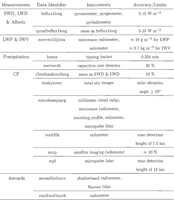
For the two sites, observations were obtained from the ARM Archive (http://www.arm. gov). Table 1.1 lists al! the datasets usecl along with a quoted observational accuracy
17 a: SGP-JJA 100 b: SGP-DJF 100 d: NSA-DJF 00 1 -&- MB
-+
VCEIL 80 ->+- ISCtp 80 --&- T81 ___ LONG ~ 60 ~ -&- MB 20-+
VCE)L 20 20 ->+- ISCCP -+- MPLo
'-_~_ _
- - - lo
'-_~_ _
- - - l oL--_~-'---_---.J 0 ' - - - - o 10 20o
10 20 o 10 20o
10 20Local Time (h) Local Time (h) Local Time (h) Local Time (h)
Figure 1.2 Mean diurnal cycle of different CF observations for (a)
sep
summer and (b) winter for 2000-03, (c) NSA summer and (d) winter for 2004.when reported. For the
sep
site, ail observations are extracted for the Central Facility (CF1) when available and if not, they were extracted from the extended facility E13. For the NSA site, ail observations come from Barrow (Cl).For the two sites, CF observations are available from many different sources. We com pared five different (different instruments or analysis) estimates for
sep
and four es timates for NSA for a corn mon period to evaluate their ability to detect the same CF and to determine a range of uncertainty in the CF observations. Figure 1.2 shows the mean diurnal cycle of three-hourly mean cloud observations, for summer and winter separately. The period forsep
is from June 2000 to December 2003, while for NSA, it covers only the year 2004. The five datasets forsep
are the CF derived from the shortwave radiation analysis of Long (stars) (Long et al. (1999», the total sky imager (squares) (Kassianov et al. (2005», the microbase cloud-radar dataset (circles) (Miller et al. (2005», the ISCCP satellite data (crosses) (Rossow et Schiffer (1991), Rossow et Schiffer (1999)) and the Vaisala ceilometer (diamonds) (Lonnqvist (1995)). For the NSA site, the four datasets are from the Vaisala ceilometer (diamonds), the microbase cloud-radar c1ataset (circles), the ISCCP satellite data (crosses) and the micropulse lidar (plus signs) (Welton et Campbell (2002».18
Table 1.1 Datasets description for observations from the SGP and NSA ~ites.
Measurements Data Identifier SWD, LWD befluxllong
& Albedo
qcrad befl ux llong LWP & IWV mwrretlliljclou
Precipitation lsmos mettwr4h
CF
15swfanalsirsllong tsiskycover microbasepiavg vcei125k isccp mplAerosols aerosolbel turn
nimfraodlmich Instruments pyranometer, pyrgeometer, pyr heliometer same as befluxllong microwave radiometer, ceilometer tipping bucket capacitive rain detector
same as SWD & LWD total sky imager
millimeter cloud radar, microwave radiometer, sounding profile, ceilometer,
micropulse lidar ceilometer
satellite imaging radiometer micropulse lidar shadowband radiometer, Raman lidar radiometer Accuracy jLimits 5-10 W m-2 5-10 Vi m-2 ;::j 18 g m-2 for LWP ;::j 0.7 kg m-2 for IWV 0.254 m~ 30 % 10 % solar elevation angle ~ 10° ma..,'( detection height of 7.5 km ;::j1O% max detection height of 18 km
19
Figure 1.2 shows that, for SGP, the Vaisala ceilometer generally underestimates CF compared to the other observations, while ISCCP tends to overestimate CF for DJF compared to the other observations. For the ceilometer, the summer underestimate is likely explained by the maximum detection height of 75 km, which leads to an under detection of upper-troposphere optically thin douds (Lonnqvist (1995)). For ISCCP, the winter differences may arise from the documented problems satellites have in distin guishing winter season low-level douds, where discrimination between a low-level cloud and snow-covered surface is difficult in the visible wavelengths, while discrimination between cloud-top infrared emission and surface emission is complicated due to the fre quent presence of a low-level thermal inversion (Key et Barry (1989); Schweiger et Key (1992)). The Long, total sky imager and microbase CF generally agree within 5-15
%
at SGP for both seasons. For this reason, we used these three datasets in our analysis, averaging the three datasets every three hours when ail three are available. If one or two datasets are not available at a given time, the datasets that are available areused as the observed CF. For the NSA site, the Vaisala ceilometer seems to match more closely the micro base dataset (clouds being generally located at a lower altitude at NSA compared to SGP means the 7.5 km height limit of the ceilometer is less of a problem), whereas the micropulse lidar seems to underestimate CF during the summer seaSOn compared to the other datasets. Based on the close agreement between the ceilometer and micro base datasets, we decided to average the three-hourly CF from these two datasets to provide the observed CF used in OlJr analysis. The reader is reminded that the CF observations do not agree and to sorne exte nt this level of disagreement should be viewed as an obser vational uncertainty (of order±
15 %) that varies with season. This level of accuracy should be borne in mind when specifie cloud-radiation parameters are analyzed and indicates the critical importance attached to accurate cloud fraction observations.20
1.3 Results
1.3.1 Large-scale meteorology
This section gives a brief overview of the model's ability to reproduce the large-scale meteorology at the two observation sites. We do this to confirm that the simulated atmosphere generally follows the observed evolution, allowing cloud-radiation processes to be evaluated against observations in a common thermodynamic phase space. 'yVe also make a preliminary analysis of the simulated 2 m temperatures at the two sites in order to later relate the impact of SRB errors on such a key variable.
As a measure of the large-scale synoptic variability, in figure 1.3 we plot the 3-day mean surface pressure and lWV for the model grid box collocated with each observation site and the same observed quantity. We choose one representative summer and winter season from the 7 to 8 years of analysis for each observation sites, other seasons being generally similar. For surface pressure, the synoptic variability is well reproduced by the model at NSA during the summer (JJA) and winter (DJF) seasons with only occasion al small biases. For sep, the variability is well reproduced by the model during the winter. Larger differences are seen at sep during the summer season, as might be expected when the model atmosphere is less constrained by the LBCs (Lucas-Picher et al. (2008)). There is no apparent systematic surface pressure bias in any of the seasons or locations. Once the model is corrected for the altitude difference at sep, the model reproduces well the observed amplitude of surface pressure for both sites and seasons. For l'yVV, the model, without any correction applied, reproduces the observed variability better in winter at both sites, also likely due to the stronger control by the LBCs in winter. In figure 1.4 wepresent the observed and simulated mean diurnal cycle of 2 m tem perature, for JJA and DJF seasons at both sep and NSA sites. These are an average over 7 years for sep and 8 years for NSA. At sep, eEM-LAM has a warm bias of ~ 5 oC through out the diurnal cycle for JJA although the actual amplitude of the diurnal cycle is well captured. At NSA, in the summer season, a nocturnal warm bias of ~ 1 oC
21
101 a: SGP-JJA 101 b: SGP-DJF 104 c: NSA-JJA ,-"-'--'--'-"'-'--'---'=:":'---, 104 d: NSA-DJF
- OSSo o 100 GEM 100 103 <il CL ,s 99 - - GEM cor. 99 98
v/'/I
\ Il -' \ r- j \ 101 101 CL 97 100 99 '---- ---.J 30 r - - - , '\ é ' 1\ \ '41
1 1 \ 20 ,,, 1 { ,1 .. 1 '\{ 10 " \ l ,1 20 \ Il , 0 0jul aug jan feb jul aug jan feb
Figure 1.3 Three-day mean surface pressure (P) and IWV al. SGP for (a) summer 2000, (b) winter 2000/01, and NSA for (c) summer 2004 and (d) winter 2004/05. For SGP, the thick dashed line represents a correction of 4.47 hPa applied to the modeled surface pressure to account for the 38 m difference in altitude between observations and mode!.
increases to 3
oC
during the afternoon period. We will subsequently indicate thal. both of these errors are strongly correlated with excess S'ND al. the surface. During the winter season, the model reproduces quite accurately the diurnal evolution of 2 m tem perature al. both locations. The SGP-JJA tempe rature error is local to central North America and does not appear linked to major circulation errors. One possi ble cause of the warm bias might be an underestimate of surface albedo, which for an accurate SWD would lead to too mach SWD being absorbed and warm the surface. Figure 1.5shows a comparison of sUlface albedo al. SGP and NSA between observed estimates (Shi et Long (2002)) and those used in GEM-LAM. In general, GEM-LAM has a realistic value of the surface albedo al. both sites although there is a failure to represent the observed di urnal cycle of surface al bedo, linked to the changing solar zeni th angle. The deviations of albedo al. SGP-JJA are certainly too small to explain the warm bias seen
22 -10 d: N8A-DJF 40 10 10 /
35 \. 5 5 -15 1 \ 1,
Ü,
~ 30 1 0 0 -20 I l 25 -5 - OBS. -5 -25 - - GEM 20 '-- - J _10'---.J -10 -30 '-- - J ~ 4 .ô~E···
.
t_GEM:j
2 .~~
:b:d'"
"
<l 0 o .~
.. .. . . ' .~...
1- 2 . ' . -2 -2 -2 -2 o 10 20 o 10 20 o 10 20 0 10 20Local Time (h) Local Time (h) Local Time (h) Local Time (h)
Figure 1.4 Mean diurnal cycle of three-hourly mean 2 m temperature for (a) SGP-JJA,
(b) SGP-DJF, (c) NSA-JJA and (d) NSA-DJF. The bottom raw shows corresponding bias.
in figure 1.4.
1.3.2 All-sky surface radiation fluxes
In this section we compare simulated and observed mean annual and mean diurnal cycles of SWD and LWD, for JJA and DJF respectively. This analysis is done for all sky conditions. A more detailed analysis follows in sections 1.31.3.4 and 1.31.3.5, where CF is used to isolate the separate raIes of water vapor or cloud liquid water on surface radiation. Figure 1.6 shows the mean annual cycle of S'ND and LWD at both SGP and NSA. GEM-LAM overestimates SWD during the spring and summer by ;:::: 15-20 W m-2 at SGP, while this overestimate is concentrated only in the summer season at NSA, but reaches ;:::: 30 W m-2 with a smaller underestimate during spring. LWD is slightly overestimated during summer at SGP (;:::: 10 W m-2
) and underestimated by a
similar magnitude in winter. At NSA, summer and fall LWD are underestimated by ;:::: 10 W m- z, while winter shows a positive LWD bias of similar magnitude. The quoted
23
0.4 a: SGP-JJA 0.4 b: SGP-DJF 0.4 c: NSA-JJA 0.8 d: N8A-DJF
- OSSo 0.3 - - GEM 0.3 0.3 0.7 - - - - . .~ -o ~ 0.2--~·
«
0.1 0 ' - - - ' 0.2 0.1 0 ' - - - '::L_'_---'
0.6 0.5 0.41
0:1
.;::
1o:~ o:~ o:~
<1-0.1
-0.1~-0.1~-0.1~
o 10 20 0 10 20 0 10 20 0 10 20
Local Time (h) Local Time (h) Local Time (h) Local Time (h)
Figure 1.5 Mean diurnal cycle of three-hourly mean surface albedo for (a) SGP-JJA, (b) SGP-DJF, (c) NSA-JJA and (d) NSA-DJF. The bot tom row shows corresponding bias.
observation al accuracy of SWD and LWD are
±
10 W m-2 and±
5 W m-2 respectively. To better understand the source of errors in the SWD and LWD annual cycles, we begin by constructing mean diurnal cycles of SWD and LWD from both model and observations. Figure 1.7 shows the mean diurnal cycle of three-hourly mean SWD and LWD for summer (JJA) and winter (DJF) at both sites. The overestimate of seasonal mean SWD at both SGP and NSA is clearly associated with a developing SWD overestimate in the middle ofthe day with a ~ 40 W m-2 maximum overestimate for SGP-JJA, ~ 30 W m-2 for SGP-DJF and ~ 50 W m-2 for NSA-JJA.Positive and negative biases seen in the mean annual cycle for LWD are also visible through the diurnal cycle during JJA and DJF. For SGP-JJA, the overestimate is maximum (~ 15 W m-2) in early afternoon and stays posiive for the rest of the day.
The SWD overestimate seen at SGP-JJA likely causes the positive 2 m temperatures bias (reasons for this will be discussed in more detail in section 1.31.3.4) and this la.ter bias is probably the direct ca.use of the LWD overestimate. The difference in
5:
200 /, / 200 05:
100 100 Cf) - OSSo - - GEM 0 0 N... 1 40 40 E 20 205:
0 0 05:
-20 -20 Cf) <l 450 450 ... 400 400 N '/ 1 E 350 3505:
300 300 p--
" O 250 2505:
n -l 200 200 (' 150 150 N... 20 20 lE5:
--
0 0 05:
- l -20 -20 <l 2 4 6 8 10 12 2 4 6 8 10 12 Months MonthsFigure 1.6 Mean annual cycle of monthly mean (a-b) SWD and (c-d) LWD at the surface for (ale) SGP and (b/d) NSA with corresponding bias.
25
800 b: SGP-DJF BOO c: NSA-JJA 800 d: NSA-DJF
- 065. ç ' 600 . 600 600 600 -:. GEM 'E ~ 400 400 o S VJ 200 200 4 0 L d J ". 20 .. . .
i::lrrl
::Im
G'.-O"'I
O· .
~O~
<l 5 0 0 , - - - . , 500 5 0 0 , - - - . , 5 0 0 , - - - , ç ' 400 400 400 400 'E 300 -=-=-,:::-=-;':";;l.-=' ~ 300 . 300 300 o ~ 200 200 200 200 f===-==-=-=-=-~~9 100 '----~---' 100 100 100 ' - - - ' 20 20 20,---~rs
0 .20 ' -_ _. ----J ·20 ' - - - ' - - - ' ·20 ' - - - ' - - - ' <l .20 0 10 20 o 10 20 o 10 20 o 10 20Local Time (h) Local Time (h) Local Time (h) Local Time (h)
Figure 1.7 Mean diurnal cycle of SWD and LWD at the surface for (a) SGP-JJA, (b) SGP-DJF, (c) NSA-JJA and (d) NSA-DJF with corresponding bias.
near-surface temperature between model and observations at SGP during the summer season (a warm bias of ::::: 5 oC as shown in figure 1.4) wou Id lead directly to a::::: 20-30 W m-2 difference in LWD, assuming surface downwelling LWD emanates mainly from near-surface emission and applying a value of 0.73-0.85 for the near-surface atmospheric emissivity (Swinbank (1963), Chen et al. (1991)). This LWD overestimate, due to near surface thermal errors, is partially balanced by a cloud underestimate at SGP-JJA (see figure 1.8 a) which acts to reduce the total sky emissivity in GEM-LAM compared to observations. For SGP-DJF and NSA-.JJA, the LWD biases also show a diurnal cycle
2
26
DJF, the overestimate of 7 W m-2 is constant through the diurnal cycle but is within the observational uncertainty (Shi et Long (2002)).
1.3.3 Cloud fraction
Simulated cloud coyer plays a key role in determining overall biases in SRB. In order to evaluate the full range of processes controlling the model SRB, it is necessary to first analyze the simulated and observed cloud fields. This is to both directly evaluate the impact of cloud errors on the total SRB, but also to allow for the separation of SRB errors into those directly associated with CF and those attributable to errors in either clear sky radiation (e.g. aerosols or water vapor impacts on radiation fluxes) or overcast radiation (e.g. representation of cloud reflection and/or cloud-radiation scattering/absorption). An analysis of all these three components, that each contribute to the all-sky SRB, will aid in identifying specifie parameterization terms requiring improvement in GEM-LAM.
Figure 1.8 shows the mean diurnal cycle of three-hourly CF, separately for JJA and DJF, at SGP and NSA. The observed CF is an average of the estimates (Long/TSI/MB for SGP and Vceil/MB for NSA) shown in figure 1.2. We remind the reader that a degree of uncertainty exists regarding the absolute accuracy of the observed CF, of
±
15%.
GEM-LAM generally underestimates CF, ranging from ~ 10%
at SGP for summer and winter, to ~ 20%
at NSA in JJA. In the winter season GEM-LAM overestimates CF at NSA by ~ 25%.
It is weil established that most observational platforms have difficulty in detecting' optically thin clouds that may be quite frequent at NSA in the winter. Wyser et Jones (2005) showed that by filtering modeled clouds to preclude all clouds with an optical thickness of less than 0.5, the resulting model CF was reduced by ~ 20-25%
in the winter season over the Arctic. Futhermore, Karlsson et al. (2008) determined that the minimum cloud optical thickness detection limits for the Advanced Very High Resolution Radiometer (AVHRR) satellite are 1.0 and 3.0 for low-level clouds at night and twilight respectively. Therefore, the NSA winter cloud bias in GEM-LAM should be treated with sorne caution. Figure 1.9 shows a normalized frequency distribution27
20
100 a: SGP-JJA 100 b: 100 c: N8A-JJA 100 d: N8A-DJF
1 - - ~ - OBS. 80 - - GEM 80 80 r---~- 80 ~ 60 60 60 """
-
-
.-
.. "--
60 .c:...- , -
-~~ LL 40 ---./"~-~ 40 40 40 Ü ' --
'-:-.-
.--.
-- 20 20 20 0 ' - - - ' O'---.J 0 0 2 0 g 2 0 C · · · 2 0 [ : J.~~12
o . . 0 0 .. . <l -20 .. . -20 . -20 .. ... . . -20 . o 10 20 Local Time (h) o 10 20 Local Time (h) o 10 20 Local Time (h) o 10 20 Local Time (h)Figure 1.8 Mean diurnal cycle of CF for (a) SGP-JJA, (b) SGP-DJF, (c) NSA-JJA and (d) NSA-DJF. The light shaded zone around the observed curve represents a degree of uncertainty regarding the absolute accuracy of the plotted observed CF (± 15 %). The bot tom row shows corresponding bias.
of 3-hourly mean CF occurrences at SGP and NSA. "YVhile the general shape of the frequency distribution is weil captured by GEM-LAM, the smail underestimate in SGP clouds appear mainly due to an overestimate of clear-sky (CF ~ 10 %) occurrences along with an underestimate of fractional cloud occurrences suggestive of an inability to simulate to simulate weakly forced convection in the summer over SGP. At NSA, the JJA underestimate in the mean CF is more a result of an underestimate of the occurrences of overcast conditions (CF ::::90 %).
The direct radiative effect of the
CF
underestimate at SGP in both seasons and at NSA in JJA, should be an underestimate of LWD and an overestima.te of SWD. However, CF is not the only factor influencing the diurnal cycle of SWD and LWD. The clearest example of this can be seen for the overestimate of LWD during the summer season at SGP, even though CF is underestimated. To remove the direct influence of CF errors, in the following sections we analyze SWD and LWD separately for clear-sky and overcast conditions. 'Vith this method, we <:an better evaluate the physical processes controlling28
a: SGP-JJA b: SGP-DJF '00 '00 _OBS . • GEM 80 80 ... ... ~ ~ a> a> u u 60 60 u~
~
0 0 E E 40 40 u u '" c '" a> ~ => => cr ~ 20 ... a> 20 IL 0:: 80 c: NSA-JJA d: NSA-DJF '00 '00 80 80 ~ ~ a> a> u c ~ 60~
60 u u 0 0 E E '" 40 '" 40 ~ ~g-
g
o:: 20 .. 0:: 20 30 40 50 60 70 80 90Cloud Fraction ('Y,)
Figure 1.9 Frequency of occurrence of 3-hourly mean CF for (a) SGP-JJA, (b) SGP DJF, (c) NSA-JJA and .(d) NSA-DJF.
29
the overcast and clear-sky radiation fluxes in GEM-LAM and compare simulated rela tionships to those seen in the equivalent observations. Once we have a better idea of the model performance in these two regimes, in combination with the CF errors, we will be in a better position to attribute errors in the simulated SRB to the representation of specifie processes in the mode!.
1.3.4 Surface radiation fluxes for clear-sky conditions
In this section we analyze surface radiation fluxes for clear-sky conditions only (CF S;
10 %). In this manner we can compare the representation of LWD and SWD fluxes isolated from the confounding effects of either CF or cloud-radiation parameterization errors.
Figure 1.10 shows the mean diurnal cycle of SWD and LWD for clear-sky conditions, this should be compared to figure 1. 7 which shows the same quantities for all-sky conditions. The overestimate of total SWD for all-sky conditions is significantly reduced when only clear-sky conditions are considered. For SGP-JJA, the all-sky SWD overestimate of~
40 W m-2 is reduced to below 20 W m-2 around local noon. Whereas, for SGP-DJF,
the all-sky SWD overestimate now becomes an underestimate, of ~ 20 W m-'l around local noon. Thus the simulated S\VD in clear-sky conditions is not the main cause of the overestimate of all-sky SWD seen in figure 1. 7, in fact the clear-sky errors tend to act in an opposite sense to the all-sky errors.
For LWD in clear-sky conditions at SGP, the same biases as LWD for all-sky conditions are seen, suggesting the LWD biases are largely controlled by near-surface temperature errors. For NSA-JJA, LWD in clear-sky conditions shows an overestimate of the diurnal cycle by the model resulting in a maximum overestimate of;:::; 15 W m-2 in the late afternoon. This clear-sky error is also likely tied to the near-surface warm bias at NSA-JJA which peaks in the late afternoon (figure 1.4) and appears directly caused by the excess all-sky SWD (figure 1.7). In terms of the all-sky LWD at NSA-JJA, the clear-sky overestimate in 1WD is not seen because of the significant underestimate in
---30 800 . 800 800 800 ..· -..OBS N - GEM E 600 600 600 600 S
0
400 400 . 400 . 400 . S (/) 200 200 200 200 oL - L -_ _- - - ' " - ' o L . - L -_ _---'"---J o L . - - - . . . - - I o L.-_-=::::=.._---J...••..•....
::[7CJ
: : 5 2 j "
-20 .. ..1~6
:::~
~~IG;:
1
<l -40 -40 500 r - - - , 500 r - - - , 500 r - - - , 5 0 0 r - - - , ...--
"!~ 400 //-
400 400 400 E ~ 300 . 300 300 300 0 ~ 200· 200 200 200 100 100 100 100 N E 20 20 1 . 20 ~ 0 0 o . S --1 <l -20 -20 -20 -20 0 10 20 0 10 20 0 10 20 0 10 20Local Time (h) Local Time (h) Local Time (h) Local Time (h)
Figure 1.10 Mean diurnal cycle of SWD and L\ND at the surface for clear-sky condi tions for (a) SGP-JJA, (b) SGP-DJF, (c) NSA-JJA and (d) NSA-DJF with correspond ing bias.
CF (peaking at ;::::: 25
%
in the afternoon), leading to an overall underestimate of all-sky emissivity, which completely offsets the thermal contribution to the clear-sky LWD. The final result being a negative bias in all-sky LWD at NSA-JJA. For NSA-DJF, the all-sky LWD positive bias of;::::: 7 W m-2 increases to ;::::: 15 W m-2 in clear-sky conditions.Atmospheric water vapor is one of the principal controls on the surface radiation budget in clear-sky conditions. Figure 1.11 presents the mean diurnal cycle of IWV. GEM-LAM underestimates the IWV throughout the diurnal cycle for SGP-JJA by;::::: 3.5 kg m-2 (;:::::
31 15 b: SGP-DJF 20 c: NSA- A 10 d: NSA-DJF - OSSo N'38 18 8 .~. ~GEM 1 E 36 16 6 10 -_-../~~--.,.,.-,-,..-,-,.._ ~ ; - 34 14 4 ~ 32 30 '--- - - J 5 '--- ----J 10
o'---'
\O~
0EJ'"
12O~
.
2 -2 . .. -2 .. . .-:~
-4 -4 GEM-OSS.~
::l::-:=:::::d
-4~-<l 0 10 20 o 10 20o
10 20 o 10 20Local Time (h) Local Time (h) Local Time (h) Local Time (h)
Figure l.U Mean diurnal cycle of IWV for (a) SGP-JJA, (b) SGP-DJF, (c) NSA-JJA and (d) NSA-DJF. The bottom row shows corresponding bias.
that may gradually lead to a surface dry bias. For SGP-DJF and NSA for both seasons, GEM-LAM reproduces the observed diurnal cycle of IWV quite accurately, within the quoted observation al uncertainty of ~ 0.7 kg m-2 (Turner et al. (2007)). These sma!l underestimates of IWV may explain sorne of the SWD and LWD clear-sky errors in the model. The underestimate of IWV for SGP-JJA should lead to a clear-sky atmosphere with reduced emissivity and thereby an underestimate of LWD. Figure 1.10 shows that the warm bias in surface temperature for SGP-JJA outweighs the underestimate in IWV resulting in a positive bias in the clear-sky LWD.
To better understand errors in the simulated clear-sky SWD and LWD we present in figures 1.12 and 1.13 observed and simulated co-variability plots, between the three hourly IWV and SWD /LWD for clear-sky conditions. Figure 1.12 shows the interaction between SWD and IWV. SWD is normalized by the solar zenith angle (SZA) with a maximum of 65°, to account for the geometrical increase in optical thickness as the SZA increases, commonly referred to as the air-mass factor (Wyser et al. (2008)). GEM-LAM reproduces the observed relationship for SGP-JJA and NSA-JJA within the limits of