Comparaison et évaluation des techniques de modélisation régionale du climat avec le modèle GEM : aire limitée versus résolution variable

UNIVERSITÉ DU QUÉBEC À MONTRÉAL

COMPARAISON ET ÉV ALUATION DES TECHNIQUES DE MODÉLISATION RÉGIONALE DU CLIMAT AVEC LE MODÈLE GEM :

AIRE LIMITÉE VERSUS RÉSOLUTION VARIABLE

MÉMOIRE PRÉSENTÉ

COMME EXIGENCE PARTIELLE

DE LA MAÎTRISE EN SCIENCES DE L'ATMOSPHÈRE

PAR

MARC VERVILLE

UNIVERSITÉ DU QUÉBEC À MONTRÉAL Service des bibliothèques

Avertissement

La diffusion de ce mémoire se fait dans le respect des droits de son auteur, qui a signé le formulaire Autorisation de reproduire et de diffuser un travail de recherche de cycles supérieurs (SDU-522 - Rév.01-2006). Cette autorisation stipule que «conformément

à

l'article 11 du Règlement no 8 des études de cycles supérieurs, [l'auteur] concède

à

l'Université du Québec

à

Montréal une licence non exclusive d'utilisation et de publication oe la totalité ou d'une partie importante de [son] travail de recherche pour des fins pédagogiques et non commerciales. Plus précisément, [l'auteur] autorise l'Université du Québec

à

Montréal

à

reproduire, diffuser, prêter, distribuer ou vendre des copies de [son] travail de recherche

à

des fins non commerciales sur quelque support que ce soit, y compris l'Internet. Cette licence et cette autorisation n'entraînent pas une renonciation de [la] part [de l'auteur]

à

[ses] droits moraux ni

à

[ses] droits de propriété intellectuelle. Sauf ententè contraire, [l'auteur] conserve la liberté de diffuser et de commercialiser ou non ce travail dont [il] possède un exemplaire.»

REMERCIEMENTS

J'aimerais remerCIer mon directeur de recherche, Dr. Ayrton Zadra pour son support scientifique, sa patience et surtout pour sa très grande disponibilité

à travers

ce périple de plusieurs mois. Je tiens également à remercier mes co-directeurs, Dr. René Laprise ainsi que Dr. Bernard Dugas pour leurs commentaires et suggestions tout au long de ce projet. Le centre ESCER, pour son appui financier durant de mes études de cycle supérieur. Mme Katja Winger pour sa collaboration à régler mes problèmes informatiques. Alain Roberge et Rebecca Schneider pour leur aide vis-à­ vis la langue de Shakespeare. Finalement, merci

à ma mère pour son soutien moral et

pour ses encouragements.

TABLE DES MATIÈRES

LISTES DES FIGURES iv

LISTE DES ACRONYMES vii

LISTE DES SyMBOLES viii

RÉSUMÉ ix

INTRODUCTION 1

ABSTRACT Il

INTRODUCTION 13

1-MODEL DESCRIPTION 17

2-EXPERIMENTS AND METHODOLOGY 18

2.1 Description of the model simulations 18

2.2 Model data sets 19

2.3 Comparison of seasonal mean climatologies 19

3-RESULTS 21

3.1 Winter over North America 21

3.2 Summer over North America 23

3.3 Winter over Europe 24

3.4 Summer over Europe 26

3.5 Comparison between model and analyses over North America 27

3.6 Comparison between model and analyses over Europe 27

CONCLUSION 29

CONCLUSION 32

APPENDICE 36

FIGURES 38

LISTES DES FIGURES

Fig. 1 GEM-LAM grids over (a) North America and (b) Europe. Corresponding GEM stretched grids with areas of interest covering the same (c) North America and (d) Europe LAM's domains. Red lines indicate the equator of the rotated grids. For GEM-LAM, the surrounding pilot and blending zones are also shown (dashed lines). For clarity, only every five grid points of the original grids are shown 38 Fig.2 500-hPa geopotential height (GZ) over North America in winter: a) GEM-LAM and b) GEM-VR means (in units of dm); c) GEM-LAM and d) GEM-VR variances (in units of dm2); e) difference between means (GEM-LAM minus GEM-VR); and t)

areas where the difference between GEM-LAM and GEM-VR means exceed

significant levels of 80,90,95 and 99% 39

Fig.3 Same as in figure 2, for 250-hPa horizontal wind speed (UV) in units of mis for

means and (mlS)2 for variances 40

Fig. 4 Same as in figure 2, for total precipitation (PRECIP) in units of mm/day for means

and (mmlday)2 for variances 41

Fig. 5 Same as in figure 2, for 1.5-m temperature (T2M) in units of

oc

for means and °C2

for variances 42

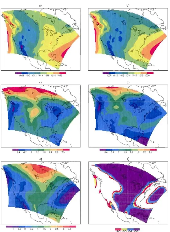
Fig.6 Same as in figure 2, for sea level pressure (SLP) in units of hPa for means and hPa2

for variances 43

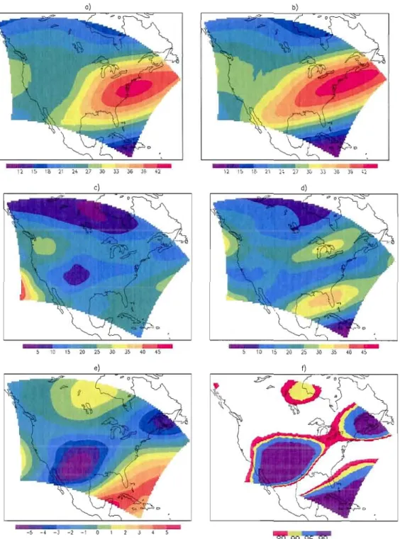
Fig.7 500-hPa geopotential height (GZ) over North America in summer: a) GEM-LAM and b) GEM-VR means (in units of dm); c) GEM-LAM and d) GEM-VR variances (in units of dm\ e) difference between means (GEM-LAM minus GEM-VR); and t) areas where the difference between GEM-LAM and GEM-VR means exceed

significant levels of 80,90,95 and 99% 44

Fig.8 Same as in figure 7, for 250-hPa horizontal wind speed (UV) in units of mis for

means and (m/s)2 for variances 45

Fig.9 Same as in fi~ure 7, for total precipitation (PREClP) in units of mm/day for means

and (mmlday) for variances 46

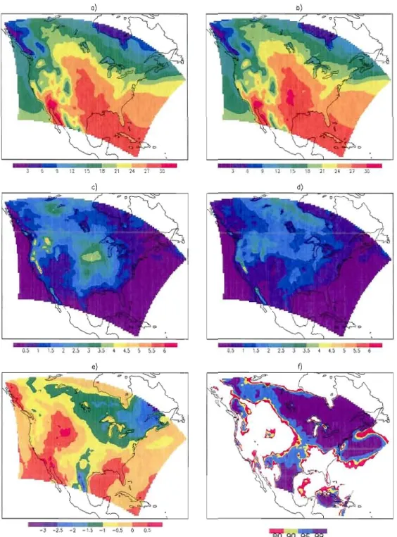
Fig. 10 Same as in figure 7, for 1.5-m temperature (TIM) in units of

oc

for means and °C2

for variances 47

Fig. 11 Same as in figure 7, for sea level pressure (SLP) in units of hPa for means and hPa2

v

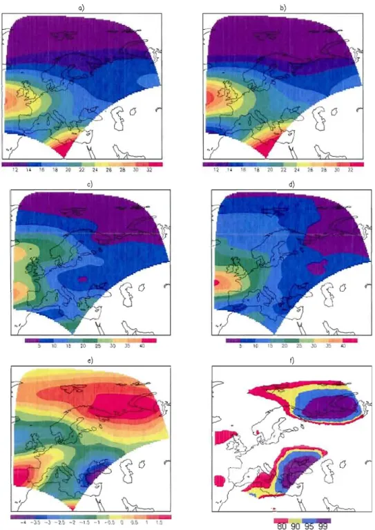
Fig. 12 500-hPa geopotential height (GZ) over Europe in winter: a) GEM-LAM and b) GEM-VR means (in units of dm); c) GEM-LAM and d) GEM-VR variances (in units of dm2); e) difference between means (GEM-LAM minus GEM-VR); and f) areas where the difference between GEM-LAM and GEM-VR means exceed significant

levels of80, 90, 95 and 99% 49

Fig. 13 Same as in figure 12, for 250-hPa horizontal wind speed (UV) in units of mis for

means and (m/si for variances 50

Fig. 14 Same as in figure 12, for total precipitation (PRECIP) in units of mm/day for means

and (mm/day)2 for variances 51

Fig. 15 Same as in figure 12, for l.S-m temperature (T2M) in units of oc for means and °C2

for variances 52

Fig. 16 Same as in figure 12, for sea level pressure (SLP) in units of hPa for means and hPa2

for variances 53

Fig. 17 500-hPa geopotential height (GZ) over Europe in summer: a) GEM-LAM and b) GEM-VR means (in units of dm); c) GEM-LAM and d) GEM-VR variances (in units of dm2); e) difference between means (GEM-LAM minus GEM-VR); and f) areas where the difference between GEM-LAM and GEM-VR means exceed significant

levels of 80,90,95 and 99% 54

Fig. 18 Same as in figure 17, for 250-hPa horizontal wind speed (UV) in units of mis for

means and (m/s)2 for variances 55

Fig. 19 Same as in figure 17, for total precipitation (PRECIP) in units of mm/day for means

and (mm/day)2 for variances 56

Fig. 20 Same as in figure 17, for 1.5-m temperature (T2M) in units of oc for means and °C2

for variances 57

Fig. 21 Same as in figure 17, for sea level pressure (SLP) in units of hPa for means and hPa2

for variances 58

Fig. 22 1.5-m temperature difference, in units of oC between simulations and ERA40 data over North America; a) GEM-LAM and b) GEM-VR in winter; c) GEM-LAM and d)

GEM-VR in summer. 59

Fig. 23 Total precipitation difference, in units of mmlday, between simulations and Xie­ Arkin data over North America; a) GEM-LAM and b) GEM-VR in winter; c) GEM­

VI

Fig. 24 1.5-m temperature difference, in units of oC, between simulations and ERA40 data over Europe; a) GEM-LAM and b) GEM-VR in winter; c) GEM-LAM and d) GEM­

VR in summer. 61

Fig. 25 Total precipitation difference, in units of mm/day, between simulations and Xie­ Arkin data over Europe; a) GEM-LAM and b) GEM-VR in winter; c) GEM-LAM

and d) GEM-VR in summer. , 62

Fig. 26 Total precipitation difference, in units of mm/day, between simulations and GEM­ UNIFORM overNorth America in summer: a) GEM-LAM and b) GEM-VR... 63 Fig. 27 1.5-m temperature difference, in units of oC, between simulations and GEM­

UNIFORM over North America in winter; a) GEM-LAM; b) GEM-VR; areas where the difference between c) GEM-LAM; d) GEM-VR and GEM-UNIFORM means

exceed significant levels 95% 64

Fig. 28 500-hPa geopotential height (GZ), in units of dm, over North America in summer: a) GEM-VR and b) GEM-UNIFORM means; c) difference between means (GEM-VR

minus GEM-uniform) 65

Fig. 29 Percentage of grids point with a significant difference between LAM and VR for a

LISTE DES ACRONYMES

ARPEGE AMIP CFL CHRM CNRM CMC CRCMD CSIRO ECMWF ESCER ESSIC FL GCM GEM HADRM HIRHAM IPCC ISBA LAM LB LBC MCG MM MMRV MRC MRCC NCAR PCMDI RCM REMO RI RPN SGMIP VR VRGCM

Action de Recherche Petite Échelle grande Échelle Atmospheric Modellntercomparison Project Conditions aux frontières latérales

Climate High Resolution Model

Centre national de recherche météorologique Centre météorologique canadien

Canadian Regional Climate Modelling and Diagnostics

Commonwealth Scientific and Industrial Research Organisation European Center for Medium-Range ofWeather Forecasts Étude et la simulation du climat à l'échelle régionale Earth System Sciences Interdisciplinary Center Frontières latérales

Global Circulation Model

Global Environnemental Multi-échelle Hadley Centre Regional Model High-Resolution Hamburg Model

Intergovernmental Panel of Climate Change Interactions Soil-Biosphere-Atmosphere Limited-Area Model

Lateral boundaries

Lateral boundary conditions Modèles de circulation générale Modèles mondiaux

Modèle mondial à résolution variable Modèle régional du climat

Modèle Régional Canadien du Climat National Center for Atmospheric Research

Program for Climate Model Diagnosis and Intercomparison Regional Climate Model

Regional Model Région d'intérêt

Recherche en prévision numérique

Stretched-Grid Model Intercomparison Project Variable resolution

LISTE DES SYMBOLES

Il

Valeur absolue

Indice d'une année

j Indice horizontal d'un point de grille

n Nombre total d'années

R Facteur d'étirement

t Valeur statistique du test de Student

u Moyenne saisonnière

V Variance biaisée

Ax Différence entre deux mailles x Moyenne climatologique saisonnière

RÉSUMÉ

Les différentes études sur les changements climatiques requièrent de ['information à plus petite échelle spatiale que les modèles globaux du climat. La modélisation régionale du climat se veut être une solution alternative pour atteindre les critères de résolutions spatiales à un coût informatique raisonnable. Les deux principales configurations utilisées pour produire des simulations climatiques à l'échelle régionale sont: le modèle à aire limitée (LAM) et le modèle mondial à résolution variable (MMRV).

Depuis quelques années, le centre météorologique canadien (CMC), plus spécifiquement la division de recherche en prévision numérique (RPN) ont façonné le modèle GEM de manière à rendre possible l'utilisation de l'une ou l'autre de ces deux configurations avec exactement les mêmes paramétrages physiques et le même noyau dynamique. En utilisant le modèle GEM, il est maintenant possible de comparer proprement les deux techniques de simulation régionale du climat. En sachant que les MMRVs requièrent un coût informatique bien au-delà de ce que demandent les LAMs, l'idée de mettre en évidence les bénéfices de chaque méthode demeure incontournable.

Nous avons donc comparé deux simulations climatiques GEM-LAM (au-dessus de l'Amérique et de l'Europe), pilotées par GEM-UNIFORM, avec deux simulations GEM-VR. Les simulations GEM-VR ont été produites en prenant soin d'étirer les mailles du modèle de manière à créer des régions d'intérêts qui coïncident parfaitement avec les domaines des simulations GEM-LAM, i.e. en ayant le même nombre de points de grilles et la même résolution. Les statistiques climatiques hivernales et estivales des deux simulations à haute résolution ont été comparées par l'entremise d'une approche statistique appelée test t de Student. Par ailleurs, les moyennes temporelles de chacune des configurations ont été comparées avec des réanalyses. Bien que les différences des moyennes temporelles entre GEM-LAM et GEM-VR sont relativement petites, le test t de Student confirme que pour la plupart des variables considérées dans cette étude, les extremums de différences sont statistiquement significatifs avec un niveau de confiance égal ou plus grand à 95 %. Par contre, on remarque un plus faible pourcentage de différences significatives au-dessus de l'Europe qu'au-dessus de l'Amérique du nord, étant même à l'occasion inexistant.

Le résultat qui distingue le plus cette étude est sans aucun doute le fait que les précipitations totales simulées par GEM-LAM sont significativement supérieures à celles générés par GEM-VR. Logiquement, cet excédant d'eau ne peut qu'être occasionné par la technique de pilotage ou/et d'éponge utilisée dans cette expérience. De plus, pour ce qui est du champ de température, on remarque que GEM-LAM reproduit un climat plus chaud en hiver et plus froid en été que GEM-VR. Pour ce qui est de la comparaison avec les réanaJyses, on constate que les deux approches démontrent les mêmes faiblesses, e.g. des régions avec un biais chaud/sec et un surplus de précipitation au-dessus des montagnes.

INTRODUCTION

La modélisation est un outil très puissant pour la simulation de différents phénomènes atmosphériques. La prévision du temps à COUlt terme (1 à 5 jours) joue un rôle primordial

dans notre société en nous guidant dans la prise de décision au quotidien. La prévision saisonnière nous donne, quant à elle, un aperçu des anomalies de température et précipitation étalées sur trois mois, ce qui permet de prévenir la population à d'éventuelles sécheresses, inondations, gels, etc. En ce qui concerne le climat, les projections climatiques couvrent plusieurs décennies. Les simulateurs climatiques sont d'une importance capitale pour l'avancement des connaissances en matière d'enjeux et d'adaptation aux changements climatiques. À titre d'exemple, ils permettent d'établir des pronostics en ce qui a trait à la réponse du climat aux différents forçages anthropogéniques à l'échelle du globe, comme l'augmentation de la concentration des gaz à effet de serre et des aérosols.

Les premiers modèles à être utilisés pour étudier le comportement de J'atmosphère à l'échelle planétaire sont les Modèles de Circulation Générale (MCG), aujourd'hui appelés modèles mondiaux (MM). Ces modèles ont été développés depuis les années 60 par plusieurs centres de recherche à travers le monde. Avec l'accroissement graduel de la puissance de calcul des ordinateurs, certains MM arrivent aujourd 'hui à utiliser un découpage de la surface terrestre en mailles d'environ 125 km de côté. Néanmoins, une telle discrétisation est incapable de bien représenter la distribution géographique ainsi que d'autres processus fondamentaux (l'hydrologie des sols ou les flux de surface) influents auprès de certains climats. Or, les scientifiques sont d'avis que les diverses études sur les changements climatiques nécessitent que cette information soit bien reproduite par les modèles (lPCC, 2007). La modélisation régionale du climat constitue ainsi une solution alternative pour atteindre les critères de résolution spatiale à un coût informatique raisonnable. Différentes méthodes statistiques et dynamiques ont été mises en œuvre afin de descendre à une échelle régionale (moins de 50 km).

2

Mise à l'échelle statistique

L'approche statistique consiste à mettre en place des relations statistiques, par exemple la méthode de régression linéaire, entre des variables prédictives qui fournissent des renseignements sur i'état àe l'atmosphère à gïande échelle (souvent des analyses) et celles dites prédites décrivant les conditions à ('échelle locale (souvent des données aux stations). Une fois ces relations bien ancrées dans un modèle statistique, ce dernier peut être appliqué au climat mondial simulé afin de produire un climat régional simulé. Cette technique statistique de mise à l'écheLle n'est pas la plus populaire auprès de la communauté scientifique de modélisation régionale du climat du fait de l'absence d'interprétation physique. Les lecteurs sont invités à consulter les travaux de Wilby et Wigley (1997) pour obtenir de plus amples détails concernant cette méthode.

Mise à l'échelle dynamique

Modèle à aire limitée

En ce qui concerne les techniques dynamiques de mise à l'échelle, il existe principalement deux types de modèles. Dans un premier temps, les scientifiques ont développé un modèle régional à aire limitée (LAM pour Limited-Area Model). Ce type de modèle régional du climat (MRC) est apparu à la fin des années 80, via le travail de Giorgi et de ses collaborateurs du National Center for Atmospheric Research (NCAR). Ce simulateur correspond à un MRC à haute résolution emboîtée dans un MM à basse résolution qui selt à initialiser et à fournir les conditions aux frontières latérales (CFL) du modèle régional. Pour la plupart des modèles à aire limitée, le pilotage s'effectue de manière unidirectionnelle (one­

way nesting), i.e. que les champs météorologiques qui se développent à l'intérieur du MRC ne viendront en aucun temps influencer le comportement des CFL dictées par le modèle pilote. Il n'existe donc aucune rétroaction entre l'information régionale et mondiale. En ce sens, cette approche est considérée comme étant non interactive. Dans leurs récents travaux, Jones et al. (1995 et 1997) ont décelé certaines incohérences entre les grandes échelles du MRC et celles du modèle pilote. Plus spécifiquement, ils montrèrent que, pour certaines

3

simulations climatiques munies d'un domaine relativement grand, l'écoulement moyen et la variabilité à l'intérieur du MRC peuvent diverger de ceux produits par le MM. Ainsi, ils recommandent que cette méthodologie soit retravaillée en profondeur. Ils suggèrent brièvement trois solutions: (i) conserver un modèle à aire restreint unidirectionnel, mais en réduisant les dimensions du domaine, de façon à mieux contrôler la circulation à grande échelle à l'intérieur du MRC et, ainsi, disposer d'une meilleure connexion entre le MM et le MRC; (ii) introduire une technique de pilotage bidirectionnel (two-way nesting) qui se discerne par une dépendance du pilote vis-à-vis le MRC et inversement (Lorenz et Jacob, 2005); et (iii) utiliser un MM avec une résolution variable, comme dans l'étude de Déqué et Piedelievre (1995). Par ailleurs, toujours dans cette même optique, von Storch et Langenberg (2000) ont développé une technique de pilotage des grandes échelles (aussi appelée pilotage spectral) qui est utilisée dans plusieurs modèles à aire limitée, dans le but de forcer ces derniers à suivre fidèlement leur pilote. Notons que cette approche s'applique seulement si la taille du domaine est assez grande. Les lecteurs sont invités à se référer à von Storch et al. (2000), Binner et al. (2000) et Miguez-Macho et al. (2004) pour une revue plus détaillée de cette méthode.

Bien que les deux premières suggestions de Jones et al. (1995 et 1997), ainsi que l'usage d'une technique de pilotage spectral, puissent être efficace pour éliminer certaines incohérences entre le MM et le MRC, il n'en demeure pas moins que les CFL constituent toujours la principale difficulté des modèles à aire limitée. En effet, l'étude du caractère «bien posé» des équations du mouvement aux CFL constitue un problème mathématique fondamental (Oliger et Sundstrom, 1978). Selon la définition d'Hadamard (1902), il est théoriquement possible d'obtenir un problème « bien posé» seulement s'il existe une solution unique, et si cette dernière dépend de façon continue des données, pour une topologie raisonnable. Or, le MRC se nourrit de CFL provenant d'un modèle ayant une résolution grossière, générant une discontinuité entre les deux modèles. Ainsi, on doit se rabattre à un problème qui n'est pas strictement « bien posé », au sens d'Hadamard, et qui ne peut être résolu que de façon discrète. De plus, les données pilote peuvent être erronées et mener à une instabilité numérique. Par conséquent, sans mécanisme de conditionnement, du bruit numérique peut facilement pénétrer à J'intérieur du MRC, à proximité des frontières

4

latérales (FL), et se propager à l'intérieur du modèle (Miyakoda et Rosati, 1977), ce qui peut potentiellement mener à une instabilité numérique (Baumhefner et Perkey, 1982). Pour éviter que le MRC soit contaminé par les CFL, il est préférable de considérer un domaine suffisamment grand, mais pas trop, de manière à ne pas contredire la première suggestion de Jones et al. (1995 et 1997). Par la suite, la façon la plus commune de corriger ce problème, i.e. le rendre bien posé, est d'introduire une zone de transition (<< zone éponge ») adjacente aux FL, dans laquelle on applique une technique de « mélange» (Davis, 1976; Robert et Yakimiw, 1986; Yakimiw et Robert, 1990). L'idée du «mélange» est de combiner l'information pilote interpolée sur la grille régionale avec celle produite par le MRC. Plus précisément, cette méthode consiste à définir une fonction de poids ayant comme rôle de modifier la valeur des champs du MRC à l'intérieur de la « zone éponge ». Cette fonction doit avoir une valeur nulle à l'entrée du domaine libre et augmenter progressivement vers la frontière latérale extérieure. L'hypothèse sous-jacente est que plus on s'éloigne des FL, plus les perturbations générées par le MRC deviennent réalistes et précises. Cette méthode peut cependant rendre instable l'équilibre dynamique de l'écoulement entrant (Staniforth, 1997). Il a été démontré cependant que cette technique est acceptable et minimise le problème des CFL (Robeli et Yakimiw, 1990).

La Fig. la et b illustre deux exemples d'une grille à aire limitée qui provient de la configuration LAM du modèle Global Environnemental Multi-échelle (GEM). Dans cet exemple, la grille est constituée en trois sous domaines: la région d'intérêt (RI) ou domaine libre; la zone de transition (<< l'éponge ») ; aussi autre région où il est nécessaire de spécifier les conditions aux limites latérales (<< zone de pilotage »). Il est à mentionner que les modèles à aire limitée ne bénéficient pas tous d'une « zone de pilotage ». À titre d'exemple, le Modèle Régional Canadien du Climat (MRCC; Caya et Laprise, 1999) est muni d'un seul point pilote en périphérie du domaine. Le modèle GEM utilise une telle configuration car il emploie un algorithme numérique semi-Iagrangien pour résoudre les équations de transport sur la totalité de la grille, incluant la « zone de pilotage» (Côté et aL, 1998a).

S'il existe certaines solutions relativement efficaces pour contrer partiellement le problème des CFL, plusieurs études en lien avec ce problème mettent en doute cette approche

5

non interactive pour modéliser le climat à l'échelle régionale. En effet, dépendamment de la situation météorologique qui prévaut, l'erreur engendrée par les CFL peut avoir un impact considérable sur ('erreur totale de la simulation. Selon Alpelt et al. (1996), ce problème joue un rôle capital en modélisation de la méso-échel1e et son importance a été souvent sous­ estimée par la communauté scientifique de méso-échelle. Pour Côté et al. (1998a), autant d'un point de vue interactif que non interactif, la méthodologie utilisée dans les modèles de méso-échelle reste à être minutieusement validée afin que ce problème soit complètement résolu.

Modèle mondial à résolution variable

La troisième suggestion de Jones et al. (1995 et 1997), qui consiste en l'utilisation d'un modèle mondial à résolution variable (MMRV), représente la deuxième approche dynamique la plus utilisée pour modéliser le climat à l'échelle régionale. Cette technique a été originalement proposée en 1977 par Schmidt pour les modèles spectraux. L'année suivante, Staniforth et Mitchell (1978) ont introduit cette idée aux MM à points de grille. Ce n'est qu'au milieu des années 90 que cette méthode a pris officiellement son envol (sous forme de configuration spectrale) via le modèle ARPEGE (Action de Recherche Petite Échelle grande Échelle) de Météo-France, autant dans un contexte de modélisation régionaJe du climat (Dequé et Piedelièvre, 1995) que dans le cadre des prévisions à courte échéance (Courtier et Geleyn, 1988 ; Yessad et Bénard, 1996). Cette technique dynamique de mise à J'échelle est aujourd'hui exploitée par plusieurs centres et groupes à travers le monde, dont Environnement Canada (Côté et al., 1998a, b) et le Earth System Sciences Interdisciplinary

Center (ESSIC) de l'Université du Maryland (Fox-Rabinovitz, 2002, 2003, 2005, 2006). Les

prochaines lignes seront d'ailleurs consacrées à la description détaillée de ce type modèle.

Comme le nom le dit, les MMRV sont des modèles mondiaux pour lesquels la résolution horizontale varie de manière à avoir une RI à haute résolution du même type que dans un modèle à aire limitée. La Fig. 1c et d illustrent deux exemples d'un MMRV tiré également du modèle GEM. La RI du modèle est représentée par un sous-domaine à haute résolution spatiale horizontale uniforme. Ce dernier est entouré d'une région d'étirement où la

6

résolution s'affaiblit graduellement pour atteindre une résolution fixe à basse résolution (résolution mondiale uniforme). Cette région à résolution variable représente une zone de transition comparable à

«

l'éponge» d'un LAM. La formulation de la grille variable peut varier d'un modèle à j'autre et cela peut avoir une influence significative sur le climat régional simulé (Fox-Rabinovitz et al., 2006).

L'autonomie d'un tel modèle représente sans aucun doute son principal atout. En effet, étant à la base un MM, le MMRV n'a pas besoin d'utiliser un autre modèle pour initialiser et nourrir sa RI. Les problèmes reliés directement ou indirectement aux CFL sont ainsi évités, mais sous certaines conditions (Fox-Rabinovitz et al., 2006). Le MMRV tire également profit d'un échange d'information bidirectionnelle entre les champs mondiaux et régionaux. Par ailleurs, les récentes études de Fox-Rabinovitz et al. (2002, 2005 et 2006) confirment l'importance de cette interaction à double sens. Bien que cette technique semble être physiquement plus réaliste que le modèle à aire limitée, quelques problèmes reliés à l'irrégularité de la grille peuvent venir entacher la solution. Par conséquent, certaines conditions quant à la configuration de la grille étirée se doivent d'être appliquées minutieusement (Vichnevetsky, 1987; Fox-Rabinovitz et al., 1988, 1997, 2006). D'abord, pour éviter des problèmes numériques, le facteur d'étirement défini comme R . = M .

lM.

l' où M. et M. 1 représentent les intervalles de deux mailles

} } j - } j

-adjacentes et j constitue l'indice horizontal, doit être uniforme (constant) et modéré. Selon Fox-Rabinovitz et al. (2006), un facteur d'étirement modéré ne doit pas dévier de l'unité de plus de 5 à 10 %. Ensuite, pour conserver une bonne qualité d'information mondiale et avoir une interaction appropriée entre les petites et grandes échelles, la distance maximale entre deux points de la grille mondiale ne doit pas être supérieure à quelques degrés, soit une distance entre 200 et 400 km. Enfin, la fine résolution au-dessus de la RI se doit d'être uniforme de manière à avoir une représentation homogène de l'orographie, du contraste terre­ mer, ainsi que d'autres forçages stationnaires en surface.

Le principal désavantage du MMRV concerne le coût informatique additionnel (par rapport au LAM), lié à son exécution, pour couvrir le reste du globe. Bien attendu, cela s'applique seulement si la simulation globale utilisée pour piloter le LAM a été exécutée

7

préalablement. Autrement, on ne peut prétendre pareil affirmation. À titre d'exemple, si on compare deux simulations issues du modèle GEM, l'une ayant été exécutée avec une configuration à aire limitée de 119 x 150 points de grille à 0.5° x 0.5° et l'autre avec une grille mondiale étirée (304 x 204), dotée d'un noyau à haute résolution de 79 x 110 points de grille à 0.5° x 0.5°, d'une résolution minimale de 1.5° x 1.5°, et d'un facteur d'étirement modéré (~7 %) au-dessus 20 points de grille, la version mondiale à maille étirée coûte environ 5 fois plus cher en temps de calcul que la configuration à aire limitée. Le MMRV demeure toutefois beaucoup moins coûteux qu'une simulation mondiale à haute résolution uniforme, soit environ 4 à 9 fois moins pour un facteur d'étirement modéré et jusqu'à 16 fois moins pour un facteur élevé. Cependant, ces gains sont très petits comparativement à ce que l'usage d'un LAM occasionne comme économie informatique (Fox-Rabinovitz, 2002, 2003, 2005 2006). Un autre inconvénient associé aux MMRVs réside dans la configuration des schémas de paramétrisations. Ces derniers doivent être en mesure de bien performer sous des résolutions spatiales pouvant varier de 40 km à 200 km.

Efficacité des techniques dynamiques de mise à l'échelle

Chacune des deux techniques (LAM et MMRV) représente une alternative de mise à l'échelle dynamique intéressante pour modéliser le climat à l'échelle régionale. Bien que ces méthodes ne soient pas parfaites, les différentes études sur la modélisation régionale du climat ont clairement démontré la qualité de ces deux configurations. Dans un premier temps, les auteurs de l'étude associée à la première phase du projet d' intercomparaison des modèles mondiaux à résolution variable (SGM1P-1; Fox-Rabinovitz et al., 2006) pour laquelle plusieurs groupes et centres ont participé (ESSIC, ESCERJRPN, CNRM et CSIRO), en arrivent aux conclusions suivantes: (1) l'approche à résolution variable semble être efficace peu importe la physique et la dynamique appliquées aux modèles, (2) ceux-ci génèrent une bonne qualité d'information régionale et mondiale, (3) la précipitation due à l'orographie semble être bien simulée, et finalement (4), ils permettent une bien meilleure représentation des forçages stationnaires en surface à l'intérieur de la RI qu'un MM standard. Pour ce qui est de la technique à aire limitée, on n'a qu'à se référer aux nombreuses études existantes (Giorgi et Mearns, 1991 ; McGregor, 1997 ; Wang et al., 2004 ; Barring et Laprise, 2005 ;

8

IPCC, 2007) pour constater ces mêmes bénéfices par rapport aux MCG. Il est donc naturel d'émettre l'hypothèse que les deux techniques de modélisation régionale du climat sont performantes à différents niveaux. En vertu des avantages et des désavantages de chacune des configurations, il est tout à fait légitime de se poser la question à savoir laquelle des deux est la mieux adaptée au cadre d'une simulation régionale du climat. Selon Côté et al. (1998a), la réponse à cette question dépend de plusieurs facteurs: la localisation géographique de la RI, la durée de la simulation, la fine résolution, les conditions météorologiques dominantes, la différence de résolution entre le pilote et le MRC, la précision de la prévision du MCG, et finalement la disposition des deux modèles dynamiques (zone de transition, facteur d'étirement, etc.).

Depuis 2004, le ,centre météorologique canadien (CMC), et plus spécifiquement la division de recherche en prévision numérique (RPN), ont façonné le modèle GEM de manière à rendre possible l'utilisation de l'une ou l'autre de ces configurations à l'intérieur même d'un seul système avec exactement les mêmes paramétrages physiques et le même noyau dynamique. Ceci constitue une première mond iale (Côté et al., 1998a, b). Ainsi, il est possible de comparer proprement les deux techniques dynamiques de simulation régionale du climat avec le modèle GEM. Cette propriété unique du GEM représente le point culminant de cette étude. Cette dernière consiste à comparer et évaluer directement les versions LAM et MMRV dans le cadre de la modélisation régionale du climat. Les objectifs sont de mettre de ['avant les avantages relatifs des deux configurations et d'approfondir les diagnostiques de comparaisons. Cette étude constitue une nouvelle approche en soi, puisqu'aucune étude de comparaison de ces simulateurs avec la même physique et la même dynamique n'a été réalisée auparavant. Il est donc difficile d'émettre des hypothèses quant aux différences et similitudes que l'on devrait retrouver.

Ce mémoire est écrit sous forme d'un article. La première partie comprend un court résumé des techniques de modélisation régionale du climat, soient l'utilisation d'un modèle à aire limitée (LAM) et l'usage du modèle mondial à résolution variable (MMRV), une brève synthèse de la conception du modèle GEM, une description de la méthodologie et une introduction à la formulation des statistiques climatiques qui seront utilisées par la suite. La

9

température à 1.5 m, les précipitations totales, la pression au niveau de la mer, la hauteur géopotentielle à 500 hPa, ainsi que le module de la vitesse du vent horizontal à 250 hPa constituent les champs météorologiques qui seront étudiés de/plus près.

Comparison of two regional climate modelling approaches using the

GEM model: global variable-resolution versus one-way nested limited­

area

Marc Yerville 1,3, Bernard Dugas 1,2,3, René Laprise 1,3 and Ayrtan Zadra 1,2,3

1 Canadian Regional Modelling and Diagnostics (CRCMD) Network, Université du Québec à Montréal 2 Numerical Prediction Reseach (NPR), Environment Canada

3 Centre pour l'étude et la simulation du climat à l'échelle régionale (ESCER Center)

Octaber 2010

Corresponding author address:

Marc Verville

Dép. Sciences de la terre et de l'atmosphère Université du Québec à Montréal (UQAM) 201, President-Kennedy Avenue, 6thfloor Montreal, QC, Canada, H2X 3Y7

ABSTRACT

Various climate-change studies ind icate the need of spatially detailed information at much finer scales than those currently resolved by Global Circulation Models (GCMs). Regional climate models (RCMs) offer a viable solution, as they are able to resolve mesoscale features over a region of interest at a computationally affordable cost. Variable­ resolution stretched-grid general circulation models (VRGCMs) and nested limited-area models (LAMs) provide two alternative and popular approaches often used in regional climate simulations.

For climate applications, a potential drawback of the one-way nesting approach used in LAMs is that it may lead to inconsistencies between the weather simulated by the regional (driven) and global (driving) models. An adequate treatment of lateral boundary conditions (LBC) in LAMs also remains a major issue (Jones et al. 1995, 1997). On the other hand, VRGCMs allow high-resolution climate simulations without any LBC updates or sudden discontinuity in resolution, and continuous two-way interaction between global and regional scales. However, the VRGCM approach cornes with a higher computational cost than that of the one-way nested technique.

The Canadian Global Environmental Multiscale (GEM) model supports both global variable and limited-area grid configurations, with the same dynamical core and physics package, and thus provides an ideal setup to compare the relative benefits of the two approaches to regional climate modelling. This study provides a comparison between these two methods using the GEM model. Two pairs of regional climate simulations, covering the period of March 1979 to February 2002, have been chosen as a benchmark for this comparison: one pair of LAM and VRGCM simulations over Europe, and one over North America. The high-resolution areas of the GEM-VR grids were chosen to coincide perfectly with those of the corresponding GEM-LAM open domains.

12

This study focuses on statistical diagnostics applied to climatological fields generated by VRGCM and LAM, namely seasonal (winter and summer) means and variances and estimates of significant differences based on the Student's t-test. Five fields have been considered: 1.5-m temperature, total precipitation, sea level pressure, horizontal wind speed at 250 hPa and geopotential height at 500 hPa. A comparison between simulations and reanalyses is also presented.

Despite overall similarities, Student's t-test results show significant differences between the climatologies of two models/approaches over large fractions of both domains, especially in the summer and more notably over North America than Europe. The total precipitation simulated by the GEM-LAM is significantly higher than that generated by the GEM-VR, regardless of season or the domain considered. Logically, this excess of water can only be created by the driving technique and/or the blending zone used in this experiment. Concerning the temperature field, it is interesting to note that the GEM-LAM produces a warmer climate in winter and a cooler climate in summer than the GEM-VR. When compared to reanalyses data, both approaches show similar weaknesses, e.g. too warm/dry regions and excessive precipitation over mountains.

INTRODUCTION

Various climate-change studies indicate the need of spatially detailed information at much finer scales than those currently resolved by General Circulation Models (GCMs). Regional Climate Models (RCMs) have been used as an alternative to high-resolution GCMs that are computationally expensive to integrate at such fine spatial resolutions. RCMs are able to resolve mesoscaJe features over a region of interest, at a computationally affordable cost. They typically have horizontal resolution of less than 50 km that allows a better representation of the orography as weil as other physical processes such as soil hydrology and surface flows when compared to a standard GCM.

The so-called one-way nested approach has become the most popular technique that allows high-resolution regional climate simulations. This downscaling technique consists in a limited-area model (LAM) whose lateral boundary conditions (LBC) come from lower­ resolution data, such as GCM simu lations or reanalyses data. The expression "one-way" means that meteorological fields generated by the RCM will not exert influence on the driving model that supplies the LBe. LAMs were first introduced in the late 80's following the seminal work of Giorgi (Giorgi and Bates 1989) at the National Center for Atmospheric Research (NCAR). This approach is now used by several climate modelling groups around the world, including the Canadian Regional Climate Modelling and Diagnostics (CRCMD) Network that developed several versions of the Canadian Regional Climate Model (Caya and Laprise 1999).

The appropriate specification of the LBC and their related fundamental issue of mathematical well-posedness (O/iger and Sundstrôm 1978) represent a significant challenge for the one-way nested modelling approach. The high-resolution LAM is driven by a global model with a coarse resolution, which creates a discontinuity at the lateral boundaries (LB) and results in an ill-posed discrete problem (Staniforth 1997). Consequently, without any adjustment, numerical noise could extend into the regional domain and propagate upstream (Miyakoda and Rosati 1977), leading eventually to computational instabilities (Baumhefner

14

and Perkey 1982). However, it was shown that the lateral boundary problems can be reduced by using a buffer zone (sponge zone) where blending and diffusion are applied (Davis 1976; Robert and Yakimiw 1986, 1990). For climate applications, a potential drawback of the one­ way nesting approach is that it may lead to inconsistencies between climates of the regional (driven) and global (driving) models (Jones et al. 1995, 1997). In some simulations, especially those using a large domain, the mean flow and the variability in the RCM may differ from that of the GCM on the synoptic scale. Some workable solutions to minimize this divergence have been proposed such as: reducing the domain size (Jones et al. 1995, 1997), introducing two-way nesting (Lorenz et Jacob 2005), and using large-scale nudging (von Storch and Langenberg 2000, Binner et al. 2000, Miguez-Macho et al. 2004). Although some of these procedures may be successful for specifie applications, the Jateral boundary conditions (LBC) remain the major difficulty of any nesting approach.

An alternative to the one-way nested-grid approach to simulate regional climate consists in using a variable-resolution GCM with enhanced high-resolution over the region of interest. This technique was originally developed by Schmidt (1977) for spectral models, and by Staniforth and Mitchell (1978) for grid point mode!s. In this approach, the resolution outside of the area of interest decreases gradually until it reaches a uniform resolution typical of global models. The formulation of the variable grid can differ from one model to another one and it may have a significant influence on the simulated regional climate (Fox-Rabinovitz et aL, 2006). This technique allows the possibility of performing high-resolution climate simulations without any LBC updates or any sudden discontinuity in resolution. Furthermore, this method includes suitable two-way interactions between global and regional scales. In the 90's, the variable-resolution configuration was implemented in the ARPEGE mode! of Météo-France, both for regional climate modelling (Déqué and Piedelièvre 1995) and for short-term weather forecasting (Courtier and Geleyn 1988; Yessad and Bénard 1996). Variable-resolution stretched-grid general circulation models (VRGCMs) are used nowadays by other centers around the world such as Environment Canada (Côté et al. 1998a, b) and at University of Maryland (Fox-Rabinovitz et al. 2006).

15

Although variable-resolution GCMs (VRGCMs) may seem to be physically more realistic than the limited-area models, sorne problems related to the non-uniformity and anisotropy of the computational grid can result in an erroneous solution. Thus, sorne strict conditions must be applied to the configuration of the stretched grid (Vichnevetsky 1987; Fox-Rabinovitz et al. 1988, 1997, 2006). First, to minimize numerical problems, the local

stretching factor R. = ilX . /ilX . 1 (ilX. and ilX. 1 are adjacent grid intervals and j is

j j j - j j

-the horizontal index) should be kept constant and moderate. According to Fox-Rabinovitz et al. (2006), a moderate stretching factor should not deviate from 1 more than 5 to 10%. In addition, to preserve a good quality of global information and an appropriate interaction between the small and large scales, the recommended maximum grid spacing should not exceed a few degrees, which corresponds to a spacing of 200-400 km. Also, the high resolution over the regional area of interest should be uniform to provide a homogeneous representation of orography and land-sea contrast as weil as of other stationary forcings.

Regarding computational costs, the VRGCM option is generally more expensive than the one-way nested technique due to its global domain. Obviously, this affirmation is true only if the driving simulation was already done before running the LAM. For instance, if we compare two 26-year simulations of the Global Environmental Multiscale (GEM) model, the one using a LAM grid over a computational domain of 119 x 150 grid points at 0.5° x 0.5°, and the other using a global variable-resolution grid (304 x 204) with a high-resolution core of 79 x 110 grid points at 0.5° x 0.5°, stretching up to a minimum resolution of 1.5° x 1.5°

with a stretching factor of ~7, the computation cost of the latter is approximately 5 times

larger than the former. Another weakness according to the VRGCMs is that the physical parameterizations must weil perform under either a 20-km or 400-km resolution grid.

The Stretched-Grid Model Intercomparison Project, phase 1 (SGMlP-l), has shown that VRGCMs are able to produce regional and global information of good quality regardless of details in the models' physics and dynamics, and often allow a better representation of stationary boundary forcing when compared to standard GCMs (Fox-Rabinovitz et al. 2006). Similar results may be also obtained with the one-way nested approach (Giorgi and Mearns 1991, McGregor 1997, Wang et al. 2004, Barring and Laprise 2005, IPCC 2007). Even

16

though the LAM and VRGCM downscaling methods are not perfect, various studies have clearly shown the benefits of using either option when compared to low-resolution GCMs. The question is: Which method is the most appropriate for regional climate modelling?

According to Côté et al. (1998a), the answer to this question depends on several factors such as: the size and the geographical location of the area of interest, the forecast period, the resolution, the prevailing weather conditions, the difference in resolution between driving and driven model, the accuracy of global forecast, and finally, the particular one-way nested or stretched-grid techniques employed (e.g. buffer zone, local stretching factor, etc.).

Recently, the Numerica1 Prediction Research Division of Environment Canada has developed the Canadian Global Environmental Multiscale (GEM) modelling system (Côté et al. 1998a, b) to run both configurations with exactly the same parameterization package and dynamical core, which provides an ideal setup to compare the relative benefits of the two approaches to regional climate modelling. The aim of this paper is to describe the results from a comparison between these two approaches using the GEM model. In the following, properties of various fields produced by regional climate simulations using LAM and VRGCM approaches are compared. A Student's t-test is performed to extract the significant difference between these two approaches. In the next section, the model configurations used to run two sets of regional climate simulations are described, and the methodology employed to analyze and compare these simulations is detailed in section 3. The main results are presented in section 4, and section 5 provides the concluding remarks.

I-MODEL DESCRIPTION

The GEM model supports three basic configurations within a single system, i.e. a global uniform latitude-longitude grid configuration, a global variable-resolution grid, and one-way nested limited-area model, allowing a flexible approach to model development. In ail configurations, we have choice to use either the fully elastic non or hydrostatic Euler equations. In our case, the fully elastic hydrostatic equations were used due to the resolutions. They are solved with a two-time-Ievel implicit semi-Lagrangian numerical scheme. The spatial discretization operates on a staggered Arakawa C-grid (Arakawa and Lamb 1977).

For the limited-area configuration, lateral boundary conditions (LBC) are provided at the surface for atmospheric pressure, and on model levels for air temperature, horizontal and vertical wind components and specifie humidity. No large-scale nudging is used, but the temperature field at the top level of GEM-LAM grids is forced to be the same as that of the driving modeI. A 10 grid-point blending region, inspired by the work of Davies (1976) and adapted by Robert and Yakimiw (1986) and Yakimiw and Robert (1990), surrounds the open domain. Furthermore, since a semi-Lagrangian numerical scheme is used all over the computational domain, the latter includes a pilot zone.

For the regional climate studies considered in this paper, the GEM model was run using the following set of physical parameterization: (i) deep and shalJow moist convective processes (Kain and Fritsch 1990); (ii) large-scale condensation (Sundqvist et al. 1989); (iii) correlated-K solar and terrestrial radiations (Li and Barker 2005); (iv) ISBA land-surface scheme (Bélair et al. 2003); (v) subgrid-scale orographie gravity-wave drag (McFariane 1987); (vi) low-Ievel orographie blocking (Lott and Miler 1997). Sea-ice coyer and sea­ surface temperature at the lower boundary have been interpolated from the PCMDI2/AMIP2

x 10 _{monthly mean climatological analyses. The AMIP2-recommended Liang and Wang} (1995) monthly ozone climatology was also used.

2-EXPERIMENTS AND METHODOLOGY

2.1 Description

of the model simulations

As a first step, a global uniform configuration of GEM (GEM-UNIFüRM) was integrated from January 1978 to February 2004 with a 3600-s (l-h) time step. The horizontal resolution was fixed at 1.5° x 1.5°, the top of the model at 2 hPa with 60 hybrid unstaggered levels in the veltical, and the domain included 240 x 120 grid points.

The output of this global simulation provided the lateral boundary conditions (LBe) to two limited-area high-resolution regional simulations (GEM-LAM), one over North America (Fig. la) and the other over Europe (Fig. lb), for the period above mentioned. The lateral boundary conditions were applied at every 3 hours derived from l-hour data of GEM­ uniform by cubic (Lagrange) spatial interpolation. The GEM-LAM grids were configured with a horizontal resolution of 0.5° x 0.5° with 119 x ISO grid points, including a 10-point pilot zone and a blending zone at the boundaries, 53 hybrid unstaggered levels in the vertical, with top level at 10 hPa, and a time step of 1800 s (30 min).

A corresponding pair of variable-resolution configurations of GEM (GEM-VR) was also integrated for the same period and the same time step of the LAM. The high-resolution areas of the GEM-VR grids (Fig. le and d) were chosen to coincide perfectly with the corresponding GEM-LAM open domains, i.e. they have the same number of co-Jocated grid points, horizontal resolution and domain sizes. The resutting GEM-VR grids have a high­ resolution core of 79 x 110 grid points at 0.5° x 0.5°, stretching up to a minimum resolution of 1.5° x 1.5° with a stretching factor of ;"7% over 20 grid points, leading to a total of 304 x 204 grid points. The GEM-VR configuration uses 60 hybrid unstaggered levels in the vertical, with top level at 2 hPa.

19

2.2 Model data sets

This study focuses on seasonal (winter and summer) means and inter-annual variances generated by GEM-VR and GEM-LAM. A sequence of 23 consecutive winters (DJF =

December-January-February) and summers (JJA = June-July-August) from March 1979 to February 2002 were chosen with time series sampled at 3-hour intervals. Only the common high-resolution areas of the GEM-VR grids and the open domain of the GEM-LAM grids are considered. The common grids of both domains, North America and Europe, have 79 x 110 grid points at a resolution of 0.5° x 0.5°. In this paper, the analysis is restricted to five fields: 1.5-m temperature (T2M), total precipitation (PRECIP), sea level pressure (SLP), horizontal wind speed at 250 hPa (UV250) and geopotentiel height at 500 hPa (GZ500).

For comparison between modeJ and analysis data, two verification datasets were employed. The monthly ERA40 2.5° x 2.5° global reanalyses from the ECMWF (European Centre for Medium-Range of Weather Forecasts; Simmons and Gibson, 2000), were chosen to evaluate sorne LAM and VR regional fields, especially those having a significant difference between GEM-LAM and GEM-VR, with the exception of the precipitation field. The verification of the simuJated precipitation has been performed using the monthly 1° x 1° global analysis of Xie and Arkin (1997). Simulations and verifying data are interpolated onto common regional 2.5° x 2.5° grids for comparison with ERA40 data, and onto 1° x 1° grids for comparison with Xie-Arkin data.

2.3 Comparison ofseasonal mean climatologies

This section defines the approach chosen to compare LAM and VR seasonal

statistics of five meteorological fields, over the North America and Europe regional

domains. To estimate how significant are the differences between seasonal (winter

and summer) mean climatologies, the Student's t-test was applied. The statistical test

was conducted at each grid point using the difference between climatological

seasonal means of LAM and VR, their associated inter-annual variance and the

sample size (which is 23, in this case). In our study, the Student's t-test is applied

-

-20

with four significance levels: 80, 90, 95 and 99 %. A statistical value

t

called "test statistic" is calculated at each grid point from the difference between climatological seasonal means (x) of LAM and VR, their biased variance (V) and the sample size (n ): t

=

X LAM - X YR _Wlt . h V _{= -}1

~(

_{~ U} - 2 i -x) n i=! V_LAM + V_YR n-l

3-RESULTS

ln this section we discuss the differences between the 23-season mean and inter-annual variance from the GEM-LAM and GEM-VR simulations, for the 500-hPa geopotentiel height (GZ), 250-hPa wind speed (UV), total precipitation (PRECfP), 1.5-m temperature (T2M) and sea level pressure (SLP) fields. Fig. 2 to fig. 21 show that the 23-seasonal mean and variance patterns obtained from the GEM-LAM and GEM-VR simulations, for ail variables above mentioned are quite similar overall. However, sorne differences can be seen, particularly in the variances of the fields GZ and UV. Although differences between means of GEM-LAM and GEM-VR configurations for ail meteorological fields are relatively smaIJ, Student's t­ tests confirm that they are statistically significant in most cases (Iess over Europe), with a high confidence level (95-99%).

3.1

Win ter over North America

Fig. 2d shows that GEM-VR has a maximum in GZ variance over the east coast, which is found fUlther east over the Gulf-Stream in the GEM-LAM simulation (Fig. 2c). Similarly, for the UV field, which represents the upper-level jet stream, Figs 3c and d show that sorne of the local maxima in variance are located further east in the GEM-LAM simulation compared to those ofGEM-VR.

In the difference field of GZ (Figs 2e and

D,

a significant maximum of 5 dm is found over large region including the Prairies and Great Plains. A small significant minimum of -2 dm is also observed over the Gulf Stream. The other local minima, which are found over western Mexico and near in-flow lateral boundaries, are not statisticaIJy significant.

The polar jet is stronger in the GEM-VR simulation than in the GEM-LAM one, as indicated by the two significant local minima of -6 ms·1 and -5 ms" in the difference field (Figs 3e and

D

over southwestem United States and the Maritime provinces. On the other

22

hand, the GEM-LAM simulation shows stronger winds than in the GEM-VR one over the

Gulf of Mexico and Atlantic Ocean (Figs 3e and f) with a maximum reaching 6 ms-I.

Regarding precipitation, GEM-LAM tends to generate more precipitation than GEM-VR, especially near in-flow lateral boundaries, convective zones and mountainous regions. Figs 4e and f show three significant local maxima in the difference field of accumulated precipitation, including one of 4 mm/day over the Pacifie Coast and two of 1.5 mm/day over the Gulf of Mexico and the Gulf Stream. On the other hand, larger amounts of precipitation are generated by GEM-VR than GEM-LAM over the NOlth-Atlantic coast and east of the Great Lakes, where two significant minima of -1 mm/day and -O.S mm/day are observed. The east of the Great Lakes is known for its large amounts of snow in winter, associated with the lake effect. Notice that precipitation variances are relatively small (Figs 4c and d) in this region, which explain why the differences in precipitation means are significant.

GEM-LAM simulation shows warmer l.S-m temperature means than GEM-VR for most of the continental domain, as indicated by the vast region of significant positive differences centered over the Rockies and reaching a maximum of 4 oC (Fig. Se). This region of positive differences is correlated with the large zone of positive differences between means of the GZ

field (Figs 2e and f). We note that the significant differences between the means of the GEM­

LAM and GEM-VR (Fig. Se and f) highly resemble the differences between the GEM-VR

and GEM-UNIFORM (Fig. 27b and d). This is not the case for the GEM-LAM and its diving mode!. There is thus a high likelihood that the differences between the two configurations are directly linked to the driving mode!. So, the warmer data in the GEM-LAM compared to the GEM-VR seems to result in part from its driving mode!.

Finally, for SLP differences, Figs 6e and f show three significant maxima of 3 hPa, 2 hPa and 1.5 hPa over Hudson Bay, Cuba and western Mexico respectively. Moreover, there are two minima of -3 hPa and -2 hPa near in-flow lateral boundaries and over the Gulf Stream respectively. Only the first one is significant with a confidence level of 95 %. Both minima and the most part of positive differences are respectively correlated with the minima and maxima observed in the difference field

23

of GZ (Figs 2e), except for the maximum over western Mexico. The minima can be also associated with the maxima in the difference field of accumulated precipitation.

3.2 Summer over North America

Sorne results in summer are similar with those obtained in winter. First, Figs 8c and d show that sorne of the local maxima in the variance field of UV are located fUl1her east in the GEM-LAM simulation compared to those of GEM-VR. Moreover, regarding precipitation, GEM-LAM tends to generate more precipitation than GEM-VR. Figs ge and f show two significant maxima in the difference field of accumulated precipitation, including a remarkable one of 15 mmdail over western Mexico and another one of 6 mmdail over the Gulf Stream. These specific regions are known for their large amounts of rain in summer, associated with the convection. Before discussing these results it is essential to note the advantages of using a higher resolution with respect to precipitation. A higher resolution does a much better job of simulating stationary forcings responsible for precipitation relating to orography and the land-sea temperature gradient (Rabinovitz 2005). The impacts are strongest near small-scale obstacles (mountainous regions) and along coastal regions. Regions susceptible to such forcings include the west and east coasts of the United States, the Gulf of Mexico from Texas to Florida, the Rockies and the Appalachians. To better interpret these differences, the temporal means of the two configurations were also compared with those of the driving simulation. We note that the GEM-LAM generates more precipitation than its driving simulation, in contrast to the GEM-VR. This is weIl illustrated in Fig. 26a where the GEM-LAM produces up to 8 mm water equivalent more than the GEM­

UNfFORM in northeast Mexico and over the Gulf Stream. It is thus clear that the surplus of

water cannot come directly from the driving mode!. Further, the hypothesis that these

differences between the GEM-LAM and the GEM-UNIFORM are due to the difference in spatial resolution must be rejected as these d ifferences do not exist between the GEM-VR and the GEM-UNIFORM (Fig. 26b). Logically, this excess of water can be only created by the driving technique and/or the blending zone used in this experience.

24

Although similarities between winter and summer are found, there are in contrast sorne differences. First, the polar jet is stronger in the GEM-LAM simulation than in the GEM-VR one, as indicated by positive significant differences ranges between 1 mis and 6 mis (Figs 8e and f). Figs IOe and f show that GEM-LAM has colder 1.5-m temperature means than GEM­ VR for most of the continental domain, especially over the prairies and the Great Plains with a minimum reaching -4°C over Northeastern Mexico and NOliheastem Québec. T2M differences are correlated with the differences between means of the SLP field (Figs Ile and f).

FUlihermore, differences in the mean field of GZ (Figs 7a and b) show that long-wave amplitudes are greater in the GEM-LAM simulation than in the GEM-VR one. It can be made more evident by looking at their differences on Figs 7e and f, where significant maxima of 2 dm are associated with the central ridge and two significant minima of -5 dm and -3 dm with the troughs. Fig. 28 also shows that GEM-UNIFORM has greater amplitude wavethan GEM-VR. It seems to have a lost of amplitude in the stretched zone of GEM-VR.

Finally, for SLP, Figs Ile and f show three significant maxima of 4 hPa over the Hudson Bay and two of 2 hPa over Cuba and Mexico. A significant minimum of -1.5 hPa over the Gulf Stream is also observed. SLP differences are correlated with the differences between means of the GZ and T2M fields (Figs 7e and f).

3.3 Winter over Europe

ln contrast with winter over NOlih America, most of differences between the means of GEM-LAM and GEM-VR are not statistically significant, except for GZ and slightly for UV. Fig. 29 shows the percentage of grids point with a significant difference between LAM and VR for a confidence level equal to 95%. We note a weaker percentage of significant differences over Europe than over America. One hypothesis which may explain why we observe less significant differences over Europe is the orientation of the rotated grid which is positioned such that the inflow passes in a much Jess stretched out area than the grid positioned over NOlih America. The much more impressive topography in NOlih America (as

25

opposed to Europe) may equally explain this difference. Tf erroneous information is integrated inside a domain of high resolution, the error will likely be more visible in a domain with many topographie obstacles. Moreover, the dynamic over both domains is it not the same, so it is likely another explanation for this difference.

Regarding GZ, Figs 12c and d show that GEM-VR has a maximum in GZ variance over Central Europe, while GEM-LAM has a minimum of variance over this same location. Figs 12e and f show a significant minimum of -5 dm over the Alps. The same figure also shows two significant maxima of 4 dm over Iceland and Russia.

For UV, the polar jet is stronger in the GEM-VR simulation than in the GEM-LAM one, as indicated by the two minima of -4 ms·! and -2.5 ms·l in the difference field (Figs 13e) near in-flow and out-flow lateral boundaries. However, the Fig. 13f shows that the last one is only significant with a confidence level of 80 %, while the first one is with 99 %.

Although differences between means for the other variables are not very significant, there are sorne common differences with results of winter over North America. First, Figs 14e and f show that GEM-LAM tends to generate significantly more precipitation than GEM-VR over specifie regions, especially over Northwestern Spain, downstream the Alps and Scandinavian Mountains with a maximum of 2 mmday"l. Northwestern of Spain and Portugal are known for their large amounts of rain in winter, associated with the in-flow low-pressure systems.

For T2M, Figs 15e and f show that GEM-LAM has warmer 1.5-m temperature means than GEM-VR for the whole continental domain, as indicated by the vast region of significant positive differences with a maximum of 1.5 oC over Central Europe. However, in contrast with results of winter over North America, only a small region over the Alps and Central Europe show significant maxima with a confidence level of 95 %. There are not enough significant differences here to make a correlation with other fields.

26

Finally, regarding SLP, Figs 16e and f show only one significant maximum of 3 hPa in the west part of the domain located near the out-flow lateral boundaries. SLP differences are correlated with the differences between means of the GZ field (Figs 7e and f).

3.4 Summer

over

Europe

Figs 17c and d show that overall, the variance in the GZ field GEM-LAM are larger than in GEM-VR, and its maximum is found further west compared to the one in the GEM-VR simulation. Regarding UV variance, the maximum over Centra! Europe and the one over Russia in the GEM-VR simulation are found further north-east in the GEM-LAM simulation and the maximum over Central Europe is greaterin the GEM-VR simulation. For SLP, Figs 2lc and d show that GEM-LAM generally exhibits more variance than GEM-VR, especially in the north-east part of the domain.

Conceming the differences between the means of both simulations, ail results are very similar with those obtained in summer over North America, i.e. GEM-LAM has greater long­ wave amplitudes than those in GEM-VR (Figs l7e and f), its polar jet is stronger than the one in GEM-VR (Figs 18e and f), it tends to generate more precipitation than GEM-VR (Figs 1ge and f), especially over the east part of the Alps and Central Europe, and finally its I.S-m temperatures are colder than those simulated by GEM-VR (Figs 20e and f). In contrast with results of winter over Europe, these differences are statistically significant for a high confidencelevel.

For SLP, Figs 21e and fshow significant minimum of -\.5 hPa over Central Europe and a significant maximum of 1.8 hPa over the North Atlantic Drift.

The differences between means of PRECIP, T2M and SLP fields are correlated with the significant minimum over Central Europe in the difference field ofGZ (Figs 17e and f).