The 2007 rifting event in Northern Tanzania studied by C and L-band interferometry
A.M. Oyena, C. Wauthierb,c, N. d’Oreyed
aDelft Institute of Earth Observation and Space Systems, Delft University of Technology, Kluyverweg, 1, 2629HS Delft, The Netherlands bRoyal Museum for Central Africa, Leuvensesteenweg, 13, 3080 Tervuren, Belgium
cDept. ARGENCO, University of Li`ege, Sart Tilman B52, 4000 Li`ege, Belgium
dThe National Museum of Natural History, Rue Josy Welter 19, 7256 Walferdange, G.D.-Luxembourg
Abstract
July–August 2007, Lake Natron, Northern Tanzania. Part of the eastern branch of the East African Rift (EAR) is struck by a series of moderate earthquakes, culminating with a 5.9 Mw earthquake on the 17th of July 2007. Thanks to the co-operation of
several teams, active in different areas of expertise, this earthquake swarm is recognised to be the first dyking event ever captured by space-born remote sensing techniques as well as ground based measurements (Calais et al., 2008; Baer et al., 2008).
This study focuses on an in-depth analysis of the C and L-band interferograms covering this event by means of the two multi-acquisition InSAR approaches, proposed by Oyen et al. (2008). The supervised ambiguity cycle slip correction focuses on the correction of unwrapping errors in the interferogram. The second strategy, the multi-acquisition InSAR cascading based on numer-ical modelling, allows to combine interferograms from different acquisition geometries in order to improve the insights in certain complex geophysical phenomena, such as rifting events. The resulting, artificial interferograms with decreased temporal baselines show less complex deformation patterns and hence facilitate the interpretation of the deformation signal. The availability of L-band radar images, with higher coherence level and fewer phase cycles, significantly improved the interpretation. The residual interpretation of the models, however, has become more difficult compared to C-band.
Key words: East African Rift, continental rifting, radar interferometry, numerical modelling
1. Introduction
The East African Rift (EAR) is a North-South oriented ge-ological feature that runs all the way through the African con-tinent. The EAR is the result of continental stretching leading to the divergence of the African plate and is characterised by earthquakes and volcanism. This study focuses on the area in Northern Tanzania along the eastern branch of the rift. The area of interest contains a salt lake (the lake Natron) in the North-West and two main volcanoes (the Ol Doinyo Lengai and Gelai) located to the South and West of the lake respectively.
From July to August 2007 this area was struck by a seis-mic swarm centred on the southern flank of the Gelai volcano. The crisis was accompanied by renewed activity of the nearby Ol Doinyo Lengai volcano, with some unusual explosive erup-tions in September 2007. This event was captured by GPS mea-surements, a local seismic network, and by two radar remote sensing instruments on the Envisat and ALOS satellites. The GPS station, located West of lake Natron, measured a displace-ment of approximately 5.6 cm vertically and 5.7 cm horizon-tally (Calais et al., 2008). This displacement was linked to the signal captured by the seismic network, but was much larger than expected at such a large distance from the earthquake’s epicentres. The radar interferograms were able to reveal the size of the deformed area.
Based on the coherence level and deformation signal, eight potentially interesting interferograms from four different acqui-sition geometries are selected in Section 2 in order to analyse the observations. Amongst the selected interferograms, two
in-terferograms are acquired in L-band. The two multi-acquisition InSAR approaches, which are explored by Oyen et al. (2008), will be applied on this data stack in Section 4.
The results are discussed in Section 5. The supervised am-biguity cycle slip correction will be applied on two interfer-ograms, one captured by the Envisat ASAR and one by the ALOS PalSAR instruments. The results of the multi-acquisition InSAR cascading approach based on numerical modelling indi-cate that this rifting event consisted out of several dyke intru-sions on the central axis of the main graben. Furthermore, the results suggest that a magma-injection is preceded by slip on a fault plane located in the direction of the magma-displacements. Finally, some conclusions are drawn in Section 6.
2. Data availability
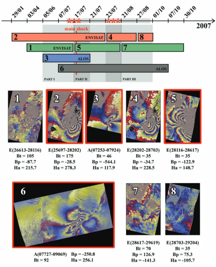
The Natron basin is monitored by both the Envisat ASAR and ALOS PalSAR instruments, providing a data set contain-ing radar images from four different acquisition geometries. Amongst these, eight potentially interesting interferograms are selected to analyse the deformation pattern and its chronology. These interferograms, including a time line, are visualised in Fig. 1. The grey bar in the time line represents the total time span of the seismic swarm, while the red stars indicate the >5 Mw single events. Based on the acquisition dates of the available radar images, the seismic swarm is subdivided into three parts. Part Iincludes the deformation at the beginning of the seismic swarm (July 12–17). Part II represents the main part of the dyking episode (July 17 – August 21) and Part III represents the deformation after the 21stof August. The main shock on
July 17th is indicated by the red vertical bar in the time line, while the interferograms containing this earthquake are marked by a red box.
Based on seismic data and more interferograms not included in Fig. 1 no deformation is assumed before July 12th and after
October 1st.
3. The supervised ambiguity cycle slip approach
High noise levels in interferograms can result in unwrap-ping errors. Unwrapunwrap-ping improvement can be applied by am-biguity cycle slip adjustment. The amam-biguity cycle slips are detected by means of peak value detection in the gradient plots along the unwrapped interferogram in both East–West and North– South directions. The outliers, or the single pixels that are se-lected to be potential unwrapping errors, will be removed and the area to be corrected will be defined. This area will be shifted up or down with respect of the rest of the interferogram by 2π or half the wavelength times an integer number. The term su-pervisedrefers to the use of a-priori information from other in-terferograms or geodetic measurements.
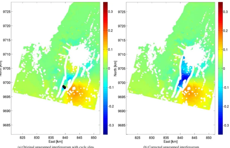
This approach is applied on interferograms 2:E(25697-28202) and 6:A(07727-09069). The corrected unwrapped interfero-grams are shown in Figs. 2 and 3. In both figures the black dots indicate the locations of the detected phase jumps. More-over, these pixels are located in the graben area in both inter-ferograms. It can be assumed that the deformation in graben areas is vertical (subsidence). This implies that the actual phase shift can be determined by cross-comparison of all the inter-ferograms, rescaled to the vertical and temporal baseline, if necessary. Therefore, the interferograms are stacked and cal-ibrated with respect to a chosen reference pixel with no defor-mation. The chosen pixel is located south-west of the lake Na-tron, where no deformation is assumed. The ambiguity number to correct for these cycle slips with is determined from a joint analysis of the cycle slip-free unwrapped interferograms and the field measurements.
Figs. 2 and 3 show that the ambiguity cycle slip adjustment is applied successfully. These optimised unwrapped interfero-grams will be used in the further analysis.
4. The multi-acquisition InSAR cascading approach based on numerical modelling
In order to improve the detailed analysis of some particular geophysical phenomena, geodetic observations are utilised as input for a modelling process. In the current study, InSAR data is used as input for a combination of the 3D Mixed Boundary Element Method (3D-MBEM) (Cayol and Cornet, 1996) and a near-neighbourhood algorithm (Sambridge, 1999a,b). The 3D-MBEM makes use of any type and number of user-defined sources. These sources are mainly fault planes with ‘slip’ or ‘opening’ or de/inflation sources. Furthermore, the 3D-MBEM method takes the topography into account, which avoids mis-interpretation of the sources in mountainous areas, as is stated by Cayol and Cornet (1998).
In order to understand this continental rifting process in more detail, each interferogram, as presented in Fig. 1, will be simulated. Due to the large temporal sampling of the radar images, the complexity of the observed displacements of such geological events as observed in northern Tanzania is too high to provide accurate and realistic models of the traditional inter-ferograms. Therefore, a method to decompose these displace-ments in smaller time periods has to be applied. The chosen method utilises several interferograms of different acquisition geometries with overlapping temporal baselines in order to cre-ate artificial, cascading interferograms.
This multi-acquisition InSAR cascading approach will be applied on Part I, Part III, and Part II respectively:
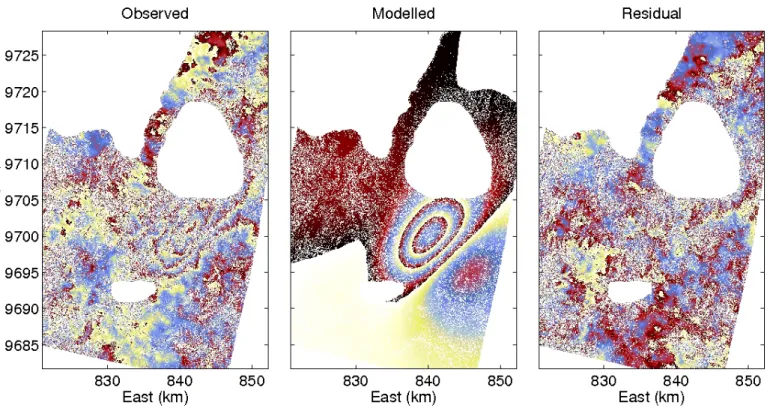
• Part I considers the deformation prior to the actual dyk-ing episode and is fully contained in interferogram 1:E(26613-28116). The model of this interferogram is referred to as artificial interferogram 12072007-17072007.
• The modelling optimisation method for Part III, which represents the deformation after the dyking episode, will be applied as follows: the oldest interferogram 8:E(28703-29204) is modelled and subtracted from interferogram 7:E(28617-29619) in order to create the artificial inter-ferogram 21082007-27082008.
• Subtracting the 12072007-17072007 deformation from interferogram 3:A(07253-07924) results in the artificial interferogram 17072007-21072007 or in Part IIa. And,
subtracting interferograms 4:E(28202-28703) and 21082007-27082008 results in interferogram 23072007-21082007 or Part IIc. The remaining Part IIb will be modelled by
three artificial interferograms simultaneously.
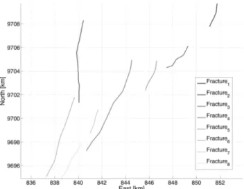
The fringe discontinuities and linear oriented decorrelated pix-els, that are observed in the wrapped interferograms and co-herence image respectively, indicate the location of the surface ruptures and are confirmed by field observations. Combining the information of these three sources resulted in the fracture map as presented in Fig. 4. These fractures will be used in the modelling process.
According to the theory (Angelier et al., 1997) and the in-formation resulting from the field observations (Delvaux et al., 2008), the geometry of the graben bounding faults is fixed dur-ing the modelldur-ing process. The dyke is assumed to be located on the central axis of the main graben and the graben bound-ing faults dip towards this central axis with a constant dip angle of 60◦. The depth of the top of the dyke is determined by the depths of the bottom of the graben bounding faults. Moreover, the dyke is assumed to be vertical. Finally, the shear stress drops on deep buried faults is fixed at 3 MPa, while on the graben bounding faults a shear stress drop of 0 MPa is consid-ered. The latter implies the passive nature of such faults as they are triggered by the stresses resulting from the dyke intrusion. 4.1. Part I
Part I, which contains the deformation prior to the dyking episode, is modelled by a 9.7 km long normal fault. The fault
Figure 1: Summary of the differential interferometric results from 29/01/2007 to 30/10/2007. Green and red indicate respectively the Envisat track 6 (swath is6) and the Envisat track 92 (swath is2) interferograms. The descending and ascending ALOS interferograms are represented by blue and black respectively. Some important parameters of the interferograms, which are named by their respective orbit numbers, like temporal baseline (Bt), perpendicular baseline (Bp) and height ambiguity (Ha) are listed next to each
interferogram. The > 5 Mw earthquakes of the seismic swarm, that started in the beginning of July 2007 and lasted up to September 2007, are indicated by the red stars on the time line. More specifically, the main shock is indicated by the vertical red line in the time line. The interferograms that contain this main shock are marked by the red boxes. The seismic swarm itself is indicated by the grey rectangle (July 2007 – September 2007).
(a) Original unwrapped interferogram with cycle slips. (b) Corrected unwrapped interferogram
Figure 2: Unwrapping adjustment of interferogram 2:E(25697-28202). The values in both the colour bars are given in meters.
(a) Original unwrapped interferogram with cycle slips. (b) Corrected unwrapped interferogram
Figure 4: Mapping of the surface ruptures by cross-comparison of the coherence image and wrapped interferogram of interfer-ogram 6:A(07727-09069) and field observations.
dips towards the northwest at an angle of 54◦with an average
slip of 1.5 m between between depths of 4 km and 5.5 km below mean sea level (MSL). The dip and strike angle were determined by the seismic data as obtained by a local seismic network, (Calais et al., 2008). The model, referred to as inter-ferogram 12072007-17072007, is shown in Fig. 6. The resid-ual phases indicate that model simulates very well the observed displacements. The residual fringes are a result of atmospheric effects and are neglected in this study.
4.2. Part II
The dyking episode is covered by Part II of the seismic swarm and is subdivided in three parts a, b, and c. Since no significant earthquake occurred between July 21 and July 23, both Part IIaand Part IIbare modelled simultaneous in order to
get a more reliable model.
Part IIaand Part IIb contain the residual deformation of
in-terferograms 2:E(25697-28202) and 3:A(07253-07924) and 12072007-17072007. The coherence image and the fringes in the wrapped interferograms indicate that Fracture4
has reached the surface and some slip occurred on Fracture7
and Fracture8. In order to simplify the model, the
geom-etry of the graben bounding faults, i.e. Fracture2/4/7/8, is
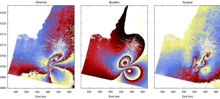
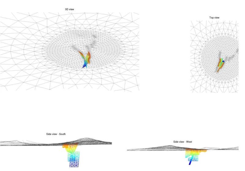
fixed. Furthermore, the model is created as a summa-tion of two separated models: (i) one covering the dyke intrusion and the slip on the graben bounding faults and (ii) another one representing the slip on a normal fault plane, which corresponds to the 17/07/2007 main earth-quake. The best fitting model suggests a dyke with an opening of 3 m at a depth of 2 km below MSL. The normal fault, associated to the main shock, has slipped 2 m in average at 3.4 km below MSL. The corresponding model is shown in Fig. 7. The residual phase in Fig. 7 indicate that the most of the observed displacements is
explained by the modelled sources. These sources are vi-sualised in Fig. 8. However, the modelled displacements near the surface ruptures deviate from the observations. The residuals also show that the displacements inside the graben area are also underestimated.
Part IIc covers the last phase of the dyking episode. During
Part IIc the western graben bounding faults, indicated
by Fracture2and Fracture6in Fig. 4, as well as Fracture4
have formed up to the surface. The model of that part IIc
is not yet considered in the present preliminary study. 4.3. Part III
The interferograms covering Part III show few fringes of deformation on the eastern and southeastern flank of the Gelai volcano. Furthermore, some slight subsidence is observed in the main graben area, which can be linked to either visco-elastic relaxation of the earth or deformation due to the cooling down of the injected magma.
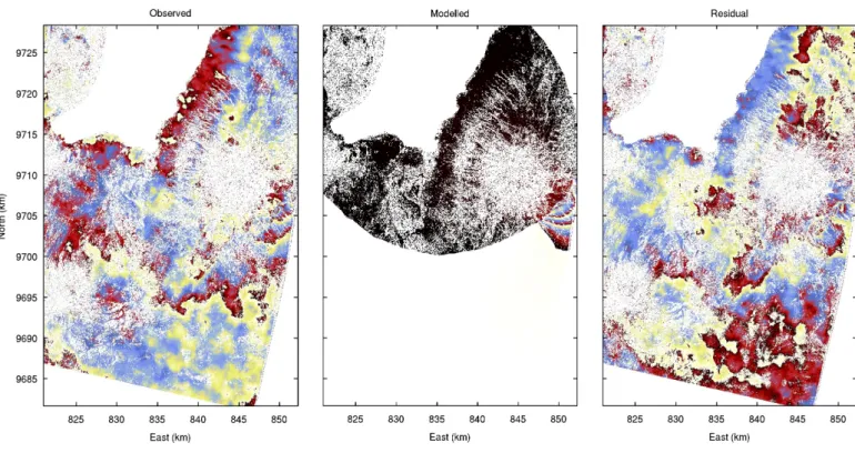
Interferogram 8:E(28703-29204) and interferogram 7:E(28617-29619) are both modelled by an east-dipping normal fault lo-cated on the southeastern flank of the Gelai volcano, with two superficial parts reaching the surface in Fracture1and Fracture3
(see Fig. 4). Since interferogram 7:E(28617-29619) is easy to interpret and it fully covers the displacements mapped in inter-ferogram 8:E(28703-29204), interinter-ferogram 8:E(28703-29204) will not be modelled in this study. However, in terms of chronol-ogy it is clear that the slip on the fault plane located on the southeast flank of the Gelai volcano migrated northwards.
The resulting model (Fig. 9) suggests an east-dipping fault with two superficial segments that reach the surface. The aver-age slip on the fault is 4 cm. According to the residual phase in Fig. 9, the model explains the main fringe pattern southeast of the Gelai volcano. However, again the fringes near the surface ruptures are not perfectly reproduced by the model.
5. Discussion
In order to validate the results that are described in Sec-tion 4 they are compared to two existing studies performed on the same case study. Since both Calais et al. (2008) and Baer et al. (2008) made use of the Okada modelling technique it is not straightforward to make a comparison between the mod-elling results. The Okada method inverts the slip on individual patches along the fault and applies a certain smoothing factor, while the 3D-MBEM superimposes a homogeneous distribu-tion of the shear stress drop on the whole fault plane and derives the global slip.
Calais et al. utilised the earthquake’s epicentres to define a main fault plane and only takes into account interferograms 1:E(26613-28116) and 5:E(28116-28617). On the other hand, Baer et al. invert the position of numerous fault planes and apply a similar method to create artificial interferograms with decreased temporal baseline.
Another difference arises from the InSAR processing soft-ware used for these studies. Baer et al. applies softsoft-ware that makes use of the raw data provided by the instruments (the
Figure 5: From left to right: observed deformation field from interferogram 1:E(26613-28116), best fit model, and residual dis-placements. (RMS: 11 mm)
JPL/Caltech ROI-PAC software and GAMMA software to per-form the ALOS PalSAR processing). Like for the current study, Calais et al. used the open source DORIS software to process the C-band and L-band data. The DORIS software makes use of the so-called Level 1 data distributed by ESA, which are the focused single look complex data. As a result of the focussing algorithm used for that pre-processing by ESA, some data are lost near the edges of the radar images and the surface covered by the SAR images are slightly smaller. Since the Gelai vol-cano is located at the near range of the radar image, part of the displacements on the eastern flank of the Gelai volcano cannot be mapped.
5.1. Part I
Interferogram 1:E(26613-28116) is modelled in all studies by a west-dipping normal fault. Both Baer and Calais suggest a similar fault depth and length of 5–10 km and 32 km respec-tively. Both studies suggest a different slip of 30 cm and 50 cm respectively. This is due to the difference in orientation of the fault plane. The results presented here suggest a fault length of 9.7 km with an average slip of 1.5 m at a depth of 4.8 km below MSL. The suggested fault plane is slightly shallower and has a length and slip which are both approximately three times as much as in the former studies. This is mainly due to the dif-ference in fault slip calculations of both the methods as stated earlier. The Okada method inverts the slip (expressed in meters) on the individual fault patches and applies a certain smoothing
factor. The 3D-MBEM superimposes a homogeneous distribu-tion of the shear stress drop on the fault plane and derives the slip. In addition the topography has a large influence on the modelled displacements in this area.
5.2. Part II
The modelling would be more accurate and reliable when multiple observations, preferably from different acquisition ge-ometries, are available. Therefore, interferograms 2:E(25697-28202) and 3:A(07253-07924) are modelled simultaneously as a single data set. This assumption is supported by the fact that Part IIbspans only two days and no significant earthquakes
oc-curred during that time.
The graben bounding faults are assumed to be fully trig-gered by the dyke intrusion, introducing the idea of passive faulting.
Baer et al. model Part IIa/bas a combination of a dyke in-trusion located in the southern part of the graben and slip on three fault planes. Two of these faults coincide with the graben bounding fault used in this study. The third fault plane is located below the Gelai volcano and corresponds to the main event on 17/07/2007. It has a length of approximately 7 km. The dyke has a length of 12 km and opens up to 1 m at a depth of 2 km. This study suggests a fault with similar length, but with a larger strike angle. The dyke has a length of 4.5 km but shows an opening of 2 m at a depth of 4.5 km. The difference between the results is remarkable in this stage. As it was the case in Part
Figure 6: Interferogram 1:E(26613-28116): Sources.
Figure 7: From left to right: observed deformation field from interferograms 2:E(25697-28202) and 3:A(07253-07924), best fit model, and residual displacements. (RMS: 37 mm)
Figure 9: From left tot right: observed deformation field from interferogram 7:E(28617-29619), best fit model, and residual dis-placements. (RMS: 25 mm)
I, this difference can be explained by the modelling techniques. The opening of the dyke intrusion as modelled by Baer et al. occurred in one main patch which is smeared out from north to south. The significant opening is only present in the northern half of the dyke. This reduces the length of the dyke to 6 km, which is closer to the result obtained by this study.
5.3. Part III
The deformation in both interferograms 7:E(28617-29619) and 8:E(28703-29204) is minor compared to that observed in the other interferograms. Therefore, Calais et al. did not con-sider these observations in the dyking episode analysis. Though, it is analysed by Baer et al.. According to their research, inter-ferogram 7:E(28617-29619) can be modelled by 5 fault seg-ments and a dyke intrusion at the location of Fracture2. Three
of these faults are not detectable in our interferograms, and the graben is not considered in Part III of the swarm.
Therefore, it can be concluded that both studies agree on the location of the fault southeast of the graben. According to Baer et al., the maximum amount of slip is approximately 20 cm, which is twice the maximum slip on the fault plane modelled in this study. However, it is not clear on which of the 5 fault planes this maximum slip would occur in Baer et al.’s analysis.
6. Concluding remarks
This study applied both the supervised ambiguity cycle slip correction and the multi-acquisition InSAR cascading approaches (Oyen et al., 2008) to the 2007 Tanzanian seismo-magmatic event. It was concluded that the second proposed strategy facil-itated the interpretation of the observed displacements. How-ever, in terms of modelling the deformation observed in the artificial interferograms was not simplified up to the preferred level. Increasing the number of sources would increase the number of parameters to invert. Therefore, in the current study several assumptions were considered for the modelling. As out-lined in Section 4, these assumptions were related to the geom-etry of the graben bounding faults and the dyke depth. The other assumptions are related to the shear stress drop superim-posed on the faults. Depending on the kind of fault, the shear stress drop is adapted. It is kept constant at a value of 3 MPa for faults related to large earthquakes or 0 MPa for graben bound-ing faults and inverted over a range of 0–10 MPa for other types of faulting.
The interferograms that span both the period prior to the dyking episode and the dyking episode itself (Part I and Part II of the seismic swarm respectively) show a remarkable tem-poral pattern. The displacements in Part I are the result of slip along a fault plane located where the dyke intrusion modelled in Part IIa/b. Furthermore, during Part IIa/band Part IIctwo
west-dipping faults, located in the northern and southern part of the graben respectively, have slipped. This behaviour indicates the occurrence of fault slip prior to the dyke intrusion as a result of the stresses imposed by the upcoming magma.
Remarkable is the northward migration of fault motion on East-dipping faults on the southeastern flank of the Gelai vol-cano. A possible hypothesis of the driving forces triggering these faults is as follows. Since these faults are neither graben bounding faults nor faults indicating any dyke intrusion/migration, their orientation implies that it is very likely that they are a re-sult of the remaining tensional forces in the earth’s crust. Due to the large surface load implied by the Gelai volcano, it is not expected that any faulting would appear on the mountain flank. However, faulting is expected at the foot of the volcano, as is observed in these interferograms.
The dyking episode that occurred at the southern flank of the Gelai volcano in the summer of 2007 was accompanied by renewed activity of the Lengai volcano. The relatively small distance between the two volcanoes suggests a most probable link between the two events. Therefore, it is preferable to per-form an InSAR time series analysis on the Lengai volcano in order to detect any deformation of the volcano or it surround-ings prior to the dyking episode. Detecting such unusual be-haviour of the earth’s surface might help to predict new mag-matic episodes and improve our knowledge about continental rifting.
Since the 3D-MBEM considers an elastic half space, the modelling of faults that reach the surface might be problematic. This is also observed in the models covering the dyking episode (Part II of the seismic swarm). An in-depth analysis the applica-tion of such faulting within the 3D-MBEM modelling method is also recommended.
Acknowledgements
The radar images presented in this study are captured in the frame of the ESA Cat-1 project CT-3224 and the ESA-JAXA ALOS project 3690. The InSAR processing was performed by the DORIS software, developed by the Delft institute of Earth Observation and Space Systems (DEOS) of the Delft Univer-sity of Technology (DUT). Orbital and topographic data are provided by DUT and SRTM respectively. The authors would like to thank P. Marinkovic for his assistance on the ALOS data processing and V. Cayol and Y. Fukushima for the use of the modelling codes and helpful suggestions.
References
Angelier, J., F. Bergerat, O. Dauteuil, and T. Villemin (1997). Effective tension-shear in extensional fissure swarms, axial rift zone of northeastern iceland. Journal of Structural Geology, 673–685.
Baer, G., Y. Hamiel, G. Shamir, and R. Nof (2008, April). Evolution of magma-driven earthquake swarm and triggering of the nearby oldoinyo lengai eruption, as resolved by insar, ground observations and elastic modeling, east african rift, 2007. Earth and Planetary Science Let-ters 272(doi:10.1016/j.epsl.2008.04.052), 339–352. Issue 1-2.
Calais, E., N. d’Oreye, J. Albaric, A. Deschamps, D. Delvaux, J. D´everch`ere, C. Ebinger, R. W. Ferdinand, F. Kervyn, A. S. Macheyeki, A. Oyen, J. Per-rot, E. Saria, B. Smets, D. S. Stamps, and C. Wauthier (2008, December). Strain accomodation by slow slip and dyking in a youthful continental rift, East Africa. Nature 456(doi:10.1038/nature07478), 783–788.
Cayol, V. and F. H. Cornet (1996). 3d mixed boundary elements for elastostatic deformation fields analysis. Int. J. Rock Mech. Min. Sci. and Geomech. Abstr. 34, 275–287.
Cayol, V. and F. H. Cornet (1998). Effects of topography on the interpreta-tion of the deformainterpreta-tion field of prominent volcanoes - applicainterpreta-tion to etna. Geophysical Research Letters 25, 1979–1982.
Delvaux, D., B. Smets, C. Wauthier, and A. S. Macheyeki (2008). Brief sci-entific report of the october 2007 field work in northern tanzania. Field mapping of the surface ruptures associated to the July-August 2007 Gelai volcano-tectonic event.
Oyen, A. M., P. Marinkovic, C. Wauthier, N. d’Oreye, and R. F. Hanssen (2008). A continental rifting event in Tanzania revealed by Envisat and ALOS InSAR observations. In ALOS PI Symposium, Rhodes, Greece, 3–7 Nov 2008, pp. 8.
Sambridge, M. (1999a, March). Geophysical inversion with a neighbourhood algorithm - i: Searching a parameter space. Geophysical Journal Interna-tional 138, 479–494.
Sambridge, M. (1999b, April). Geophysical inversion with a neighbourhood algorithm - ii: Appraising the ensemble. Geophysical Journal Interna-tional 138, 727–746.