Advanced numerical framework to simulate
Incremental Forming Processes
Thesis submitted to the University of Liège and University of Aveiro for the degree of ‘Docteur en Sciences de l’Ingénieur’
and ‘Doutor em Engenharia Mecânica’ by José Ilídio Velosa de Sena
PhD Scholarship granted by Fundação para a Ciência e Tecnologia (FCT) under SFRH/BD/71269/2010 Apoio financeiro da FCT e do FSE no âmbito do III Quadro Comunitário de Apoio.
Author
José Ilídio Velosa de Sena
Email from University of Aveiro: [email protected] Email from University of Liège: [email protected]
Supervisors at University of Liège Docteur Anne Marie Habraken
Research Director of F.N.R.S., ArGEnCo department, University of Liège Email: [email protected]
Professor Laurent Duchêne
Assistant Professor, ArGEnCo department, University of Liège Email: [email protected]
Address
MS²Fdivision, ArGEnCo Department, Université de Liège, Chemin des Chevreuils 1,
4000 Liège, Belgium
Supervisors at University of Aveiro Professor Ricardo José Alves de Sousa
Auxiliar Professor, University of Aveiro, Portugal Email: [email protected]
Professor Robertt Angelo Fontes Valente Auxiliar Professor, University of Aveiro, Portugal Email: [email protected]
Address
GRIDS Research Group, TEMA Research Unity, Department of Mechanical Engineering,
Campus Universitário de Santiago, University of Aveiro, 3810 Aveiro, Portugal
Jury members
President Prof. João de Lemos Pinto
Full Professor, University of Aveiro, Portugal
Prof. Marta Cristina Cardoso de Oliveira
Auxiliar Professor of the Faculty of Sciences and Technology, University of Coimbra, Portugal
Prof. Renato Natal Jorge
Associate Professor of the Faculty of Engineering, University of Porto, Portugal
Prof. Luis Filipe Menezes
Full Professor of the Faculty of Sciences and Technology, University of Coimbra, Portugal
Dr. Anne Marie Habraken, Supervisor of the thesis
Research Director of F.N.R.S., ArGEnCo department, University of Liège, Belgium
Prof. Ricardo José Alves de Sousa, Supervisor of the thesis
Acknowledgements Em primeiro lugar, ao Professor Doutor Ricardo José Alves de Sousa, orientador principal, o meu reconhecimento e privilégio pela oportunidade de realizar o doutoramento, sua constante boa disposição, disponibilidade, orientação, amizade, otimismo e exigência científica ao longo da preparação do trabalho, o meu sincero muito obrigado.
To Research Director of F.N.R.S, Doctor Anne Marie Habraken, supervisor at University of Liège, my appreciation for the opportunity of developing part of my research work at the University of Liège. As well as the fruitful scientific discussions in order to finish this thesis successfully.
Ao Professor Doutor Robertt Angelo Fontes Valente, co-orientador, o meu obrigado pela amizade, boa disposição, disponibilidade, otimismo, rigor científico e conselhos relevantes dados ao longo da realização do trabalho. To Professor Laurent Duchêne, co-supervisor at University of Liège, for his availability and scientific support during my stays in Liège. All the scientific discussions and ideas to identify and solve issues for the success of the numerical simulations.
To all LAGAMINE group members, for the sympathy and tasty cakes of the team meetings. In particular, to Amine BenBettaieb, Carlos Guzman and Kalipha Marmi for their friendship and scientific discussions. Also, the assistance provided at my first stay in Liège by Cédric Lequesne about technical and scientific knowledge of in-house code LAGAMINE.
To all the people which I shared social meetings with funny moments during all my stays in Liège, a special thanks.
To EURAXESS mobility centre for foreign PhD students at University of Liège for all the mobility support and stays in Liège.
Ao Tiago Almeida, José Sousa e ao Ricardo bastos, pela ajuda e colaboração na execução dos procedimentos experimentais, nomeadamente dos ensaios, produção e medições experimentais. A todos os membros do GRIDS, obrigado pelo modo caloroso como fui recebido no grupo contribuindo para a minha imediata integração, pelo bom ambiente, espírito de grupo e convívio proporcionado. Em particular, agradeço aos colegas de gabinete ao longo destes anos pela camaradagem, boa disposição e discussões científicas proporcionadas. À Fundação para a ciência e Tecnologia (FCT), por todo o apoio financeiro concebido através da bolsa de doutoramento SFRH/BD/71269/2010.
À minha família, pelo constante apoio sempre acreditando no meu potencial ao longo do meu percurso de vida. Em particular, aos meus Pais, o reconhecimento por todo o esforço, apoio e incentivo incondicional dado durante o meu percurso académico bem como em todas as etapas da minha vida, o meu maior agradecimento.
Finalmente, a todos e a cada um, que contribuíram diretamente ou indiretamente na concretização deste trabalho, a minha gratidão e reconhecimento. A todos, muito obrigado.
Keywords Incremental sheet forming; Single point incremental forming; Numerical simulation; Adaptative remeshing; Finite Element Method (FEM); Plastic deformation.
Abstract The framework of the present work supports the numerical analysis of the Single Point Incremental Forming (SPIF) process resorting to a numerical tool based on adaptive remeshing procedure based on the FEM. Mainly, this analysis concerns the computation time reduction from the implicit scheme and the adaptation of a solid-shell finite element type chosen, in particular the Reduced Enhanced Solid Shell (RESS). The main focus of its choice was given to the element formulation due to its distinct feature based on arbitrary number of integration points through the thickness direction. As well as the use of only one Enhanced Assumed Strain (EAS) mode. Additionally, the advantages include the use of full constitutive laws and automatic consideration of double-sided contact, once it contains eighth physical nodes.
Initially, a comprehensive literature review of the Incremental Sheet Forming (ISF) processes was performed. This review is focused on original contributions regarding recent developments, explanations for the increased formability and on the state of the art in finite elements simulations of SPIF. Following, a description of the numerical formulation behind the numerical tools used throughout this research is presented, summarizing non-linear mechanics topics related with finite element in-house code named LAGAMINE, the elements formulation and constitutive laws.
The main purpose of the present work is given to the application of an adaptive remeshing method combined with a solid-shell finite element type in order to improve the computational efficiency using the implicit scheme. The adaptive remeshing strategy is based on the dynamic refinement of the mesh locally in the tool vicinity and following its motion. This request is needed due to the necessity of very refined meshes to simulate accurately the SPIF simulations. An initially mesh refinement solution requires huge computation time and coarse mesh leads to an inconsistent results due to contact issues. Doing so, the adaptive remeshing avoids the initially refinement and subsequently the CPU time can be reduced.
The numerical tests carried out are based on benchmark proposals and experiments purposely performed in University of Aveiro, Department of Mechanical engineering, resorting to an innovative prototype SPIF machine. As well, all simulations performed were validated resorting to experimental measurements in order to assess the level of accuracy between the numerical prediction and the experimental measurements. In general, the accuracy and computational efficiency of the results are achieved.
I
Contents
List of Figures ... VII
List of Tables ... XV
Nomenclature ... XVII
List of Symbols (Scalars and tensors) ... XVII List of Indices... XXIV List of Abbreviations ... XXVI
Chapter 1 - Introduction ... 1
1.1 Incremental Sheet Forming (ISF) ... 1
1.2 Single Point Incremental Sheet Forming (SPIF) ... 4
1.2.1 Forming tool ... 7
1.2.2 Material and sheet thickness ... 8
1.2.3 Forming speed ... 9
1.2.4 Toolpath and vertical increment ... 9
1.2.5 Lubrication ... 10
1.3 Machinery used in SPIF ... 11
1.4 Motivation and Scope ... 13
1.5 Main objectives ... 14
II
Chapter 2 - State of the art: A review ...17
2.1 Experimental research and developments ... 17
2.1.1 Influence of SPIF parameters on the axial force ... 18
2.1.2 Force prediction ... 23
2.1.3 Twist phenomena ... 24
2.1.4 Forming tool developments ... 25
a) Free rotation ball tip ... 26
b) Comparison of Oblique Roller Ball and Vertical Roller Ball ... 26
c) Laser forming process coupled with SPIF ... 28
d) Water jet as a tool ... 28
2.1.5 Tool trajectory ... 30
2.2 Numerical simulation developments ... 31
2.2.1 Integration algorithms: Explicit and Implicit... 32
2.2.2 Finite element types ... 34
2.2.3 Constitutive laws ... 37
2.2.4 Interaction between tool and sheet ... 39
2.2.5 Domain decomposition methods ... 42
2.2.6 Adaptive refinement strategies ... 43
2.3 Formability and SPIF mechanisms ... 46
2.3.1 Analytical analyses ... 49
2.3.2 Combination of stretch, bending and shear ... 51
2.3.3 Through Thickness Shear (TTS) ... 53
2.3.4 Bending Under Tension (BUT) ... 54
2.3.5 Cyclic strain effect ... 55
III
Chapter 3 - Topics in Nonlinear Formulation ...61
3.1 Principle of Virtual Work ... 61
3.2 Continuum Mechanics ... 65
3.2.1. Deformation Gradient ... 68
3.2.2. Polar Decomposition... 70
3.2.3. Updated Lagrangian ... 72
3.2.4. Finite Element Linearization ... 73
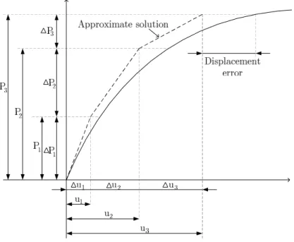
3.3 Approximate Solution: Finite Element Discretization ... 76
3.3.1. Isoparametric Space ... 79
3.4 Incremental-Iterative Procedure ... 84
3.4.1. Newton-Raphson ... 85
3.4.2. Modified Newton-Raphson... 87
3.5 Objective Stress Rate ... 88
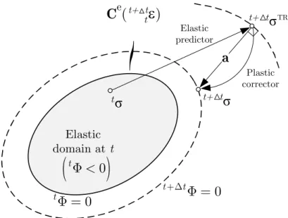
3.6 Nonlinearities ... 93
3.6.1. Geometric nonlinearity ... 93
3.6.2. Material nonlinearity ... 94
a) Yield criterion ... 96
b) Hardening behaviour ... 97
c) Plastic flow rule ... 99
d) Constitutive law integration ...100
e) Consistent elastoplastic tangent modulus tensor...102
3.6.3. Boundary Conditions: Contact Formulation ...103
3.7 Reduced Enhanced Solid-Shell (RESS): Description ...107
3.7.1. Enhanced Assumed Strain Method ...108
3.7.2. FEM approximation of the EAS method ...109
IV
3.8. Numerical Code LAGAMINE ...116
3.8.1. Pre-Processor: Generation of the “reading” files ...117
3.8.2. Processor: Simulation Processing ...117
3.8.3. Pos-Processor: Simulation Result Treatment ...119
Chapter 4 - Remeshing for SPIF: Description ... 121
4.1. Adaptive Remeshing Method ...121
4.1.1. Refinement Criterion ...122
4.1.2. Generation of New Nodes ...123
4.1.3. Generation of New Elements ...125
4.1.4. Transfer of State Variables and Stress Components ...127
4.1.5. Linked List and Cell Management: Addition of a New Cell ...128
4.1.6. Derefinement Indicator ...131
4.1.7. Removing a Cell ...132
4.1.8. Constrained Nodes: Master-Slave Method ...133
4.1.9. Boundary Conditions ...135
4.1.10. Storage Array Update of LAGAMINE ...135
4.1.11. Mesh Renumbering ...137
4.1.11.1. Seed Method or oil spot ...137
4.1.11.2. Directional Method ...137
4.2. Working Procedure in LAGAMINE Code ...138
4.3. Line Test Benchmark: Numerical Simulation ...139
4.3.1. Sensitivity Analysis of Remeshing Parameters ...140
V
Chapter 5 - Numerical tests ... 151
5.1 Simulation of incrementally formed conical shape ...151
5.1.1. Shape and thickness prediction ...155
5.1.2. Major and minor strains prediction ...159
5.1.3. Axial force prediction ...160
5.1.4. Remarks of cone shape simulations ...165
5.2 Simulation of a two slope pyramid ...166
5.2.1. Shape prediction ...169
5.2.2. Through thickness stress analysis ...175
5.2.3. Remarks of two-slope pyramid simulations ...180
5.3 Second analysis of a two-slope pyramid ...181
5.3.1. Prediction of the shape and thickness ...183
5.3.2. Major strain prediction ...185
5.3.3. Through thickness stress analysis ...186
5.4 Simulation of multistage incremental sheet forming ...188
5.4.1. Shape and thickness prediction ...191
5.4.1.1. Second analysis of multistage sheet forming ...199
5.4.2. Major strain prediction ...199
5.5 Final remarks ...203
Chapter 6 - Conclusion ... 207
6.1 Final considerations...207
6.2 Future works ...209
Appendix A - Adaptive Remeshing subroutines: Flowchart description 211
Appendix B - Yield surface influence ... 213
VII
List of Figures
Figure 1.1: Asymmetric incremental sheet forming variants. ... 3
Figure 1.2: Single Point Incremental Forming (SPIF) setup (Sena et al., 2011). ... 4
Figure 1.3: Contour a) and spiral b) toolpaths. ... 5
Figure 1.4: Wall contact with the forming tool. ... 7
Figure 1.5: Schematic representation of a) constant vertical incremental (Z) and b) constant scallop height (h). ... 10
Figure 1.6: Prototype machine for SPIF from University of Aveiro. ... 12
Figure 1.7: Standard strategy to build a toolpath for SPIF. ... 13
Figure 2.1: Variation of force curve for large wall angle values. ... 19
Figure 2.2: Grid circles distorted into ellipses and measurements orientation (Ambrogio et al., 2008). ... 20
Figure 2.3: Twist effect observed for cone and pyramid shapes (Vanhove et al., 2010). ... 24
Figure 2.4: Different topologies of forming tools tested, (a) standard hemispherical rigid tool, (b) VRB and (c) ORB (Lu et al., 2014). ... 26
Figure 2.5: Technological windows of WJ process. ... 29
Figure 2.6: Schematic representation of an alternative toolpath (Bambach and Hirt, 2005). ... 35
Figure 2.7: Geometrical assumption, parameter L limited to 5x times the tool radius. ... 41
VIII
Figure 2.8: Schematic representation of FLC in SPIF against conventional forming.
... 47
Figure 2.9: Difference between forming by stretch (left) and forming by shear (right). ... 51
Figure 3.1: General three-dimensional body and Dirichlet and Neumann boundary conditions. ... 62
Figure 3.2: Connecting relations of fields in continuum mechanics. ... 64
Figure 3.3: Position of a material point at different configurations. ... 65
Figure 3.4: Linear 8 nodes hexahedral finite element in the global and local coordinate systems. ... 80
Figure 3.5: Incremental procedure. ... 84
Figure 3.6: Standard Newton-Raphson method. ... 85
Figure 3.7: Modified Newton-Raphson method. ... 87
Figure 3.8: Schematic concept of yield surface. ... 95
Figure 3.9: Evolution behaviour of the yield surface. ... 98
Figure 3.10: Generic representation of stress return mapping procedure. ...101
Figure 3.11: Schematic contact between two bodies. ...103
Figure 3.12: Local frame work...104
Figure 3.13: Distance between contact element GP and foundation segment (lateral view). ...105
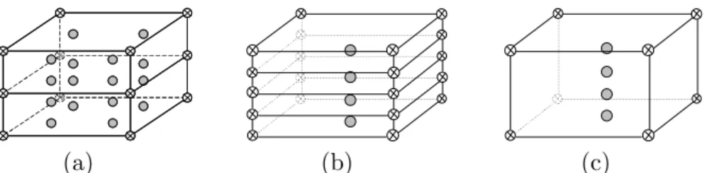
Figure 3.14 – Comparison between (a) fully integrated, (b) reduced integrated and (c) RESS formulation, regarding the number of integration points. ...108
Figure 3.15: Integration scheme in isoparametric domain with n Gauss points in the thickness direction. ...110
Figure 3.16: Procedure scheme of nonlinear LAGAMINE code. ...116
IX
Figure 3.18: Input files and generated files by LAGAMINE code. ...118
Figure 3.19: LAGAMINE code working scheme. ...120
Figure 4.1: Adaptive remeshing procedure. ...122
Figure 4.2: Generation of new nodes in element plane. ...123
Figure 4.3: Table of nodes with two layers corresponding to an eight node element. ...124
Figure 4.4: Schematic representation of new nodes table for eight node element during refinement. ...125
Figure 4.5: New elements list generation from nodes table for eight node elements example. ...126
Figure 4.6: Refined elements generation of coarse elements from new nodes table. ...126
Figure 4.7: Interpolation method scheme (Habraken, 1989). ...127
Figure 4.8: Linked list based on pointers. ...129
Figure 4.9: Addition of a new cell in the linked list. ...130
Figure 4.10: Distortion criterion, lateral view. ...131
Figure 4.11: Removing a cell from the chained linked list. ...132
Figure 4.12: Constrained new nodes generation during the mesh unrefinement. ...133
Figure 4.13: Storage array (SIGVA) update of LAGAMINE code. ...136
Figure 4.14: Flow chart of adaptive remeshing procedure in LAGAMINE in-house code. ...138
Figure 4.15: Schematic description of the experimental setup (Bouffioux et al., 2008a). ...139
Figure 4.16: Reference mesh (1) and coarse mesh (2) used with adaptive remeshing. ...141
X
Figure 4.17: CPU time and error sensitivity of forces and shape prediction for dmax
equal to 0.2 mm. ...142 Figure 4.18: CPU time and error sensitivity of forces and shape prediction for dmax
equal to 0.1 mm. ...143 Figure 4.19: CPU time and error sensitivity of forces and shape prediction for dmax
equal to 0.05 mm. ...143 Figure 4.20: CPU time and error sensitivity of forces and shape prediction for dmax
equal to 0.005 mm. ...144 Figure 4.21: CPU time and error sensitivity of forces and shape prediction for α coefficient equal to 0.1. ...145 Figure 4.22: CPU time and error sensitivity of forces and shape prediction for α coefficient equal to 0.6. ...145 Figure 4.23: CPU time and error sensitivity of forces and shape prediction for α coefficient equal to 0.8. ...146 Figure 4.24: CPU time and error sensitivity of forces and shape prediction for α coefficient equal to 1.0. ...146 Figure 4.25: CPU time and error sensitivity of forces and shape prediction for α coefficient equal to 1.6. ...147 Figure 4.26: Evolution of number of elements and nodes during the adaptive
remeshing procedure. ...148 Figure 4.27: Final number of elements for different pair combination of remeshing parameters. ...148 Figure 5.1: Forming of a conical shape: geometric dimensions. ...152 Figure 5.2: Reference mesh with 5828 finite elements used to perform a 45º wall angle cone simulation. ...153 Figure 5.3: Coarse mesh of 347 finite elements used with adaptive remeshing to perform a 45º wall angle cone simulation. ...153
XI
Figure 5.4: Final shape and thickness prediction using adaptive remeshing with α coefficient equal to 1.0 and dmaxequal to 0.05 mm. ...155 Figure 5.5: Shape prediction error and CPU time for different levels of remeshing refinement and reference mesh (corresponding to n=0). ...156 Figure 5.6: Shape and thickness predictions in the rolling direction (RD) with adaptive remeshing refinement (n=2). ...157 Figure 5.7: Shape and thickness predictions in the transverse direction (TD) with adaptive remeshing refinement (n=2). ...158 Figure 5.8: Minor plastic strain prediction. ...159 Figure 5.9: Major plastic strain prediction. ...159 Figure 5.10: Force prediction for different levels of adaptive remeshing refinement and reference mesh using the Swift hardening law with biaxial material parameters. ...161 Figure 5.11: Force prediction for different levels of adaptive remeshing refinement and reference mesh using the Voce hardening law with uniaxial material
parameters. ...161 Figure 5.12: Axial force prediction using the reference mesh with Swift hardening law. ...163 Figure 5.13: Comparison of axial force prediction obtained from different Finite Elements codes...164 Figure 5.14: Uniaxial tensile test (extrapolated). ...165 Figure 5.15: Component nominal target dimensions. ...167 Figure 5.16: Reference mesh (1) and coarse mesh used with adaptive remeshing (2). ...168 Figure 5.17: Final shape prediction in Y cut for different refinement levels after the tool unload. ...170
XII
Figure 5.18: Zoom of shape prediction at wall angle change on section A in Y cut for different refinement levels. ...171 Figure 5.19: Final shape prediction in X cut for refinement n equal to 3 nodes per edge, after tool unload. ...173 Figure 5.20: Shape prediction for X cut at different depth steps using the adaptive remeshing method. ...174 Figure 5.21: Shape prediction for X cut at 40 mm and 60 mm of depth. ...175 Figure 5.22: Position of three selected elements after contour 60 mm (1) and after contour 90 mm unloading step (2). ...176 Figure 5.23: Stress components through the thickness for the three elements at depth stage 60 mm. ...177 Figure 5.24: Simple elastic schematic representation of bending/unbending plus stretching associated to elements a) and b). ...178 Figure 5.25: Relative stress components in thickness direction for the three elements at the end of 90 mm, after tool unloaded. ...178 Figure 5.26: Experimental measurements resorting to DIC from ARGUS software. ...181 Figure 5.27: Sections measurement on the external surface of the shape...182 Figure 5.28: Final shape prediction of section AB corresponding to Y cut. ...183 Figure 5.29: Thickness prediction of section AB corresponding to Y cut. ...183 Figure 5.30: Final shape prediction of section CD corresponding to X cut. ...184 Figure 5.31: Thickness prediction of section CD corresponding to X cut. ...184 Figure 5.32: Final major strain prediction of section AB corresponding to Y cut .185 Figure 5.33: Final major strain prediction of section CD corresponding to X cut. 186 Figure 5.34: Physical meaning of out-of-plane motion. ...186 Figure 5.35: Strategy to form a vertical wall shape. ...188
XIII
Figure 5.36: Dimensions of the cone with vertical wall angle. ...189 Figure 5.37: The final vertical wall angle shape. ...189 Figure 5.38: Shapes obtained after each forming stage. ...190 Figure 5.39: Occurrence of fracture in the last contours of the last stage. ...190 Figure 5.40: Reference mesh with 3325 finite elements. ...191 Figure 5.41: Coarse mesh of 523 finite elements used with adaptive remeshing method. ...191 Figure 5.42: Shape after first stage of 50º wall angle. ...192 Figure 5.43: Thickness of the shape after the first stage of 50º wall angle. ...192 Figure 5.44: Shape after first stage of 60º wall angle. ...193 Figure 5.45: Thickness of the shape after the first stage of 60º wall angle. ...193 Figure 5.46: Measurement of cross section of 70º wall angle cone (colour lines of depth). ...194 Figure 5.47: Shape after first stage of 70º wall angle. ...195 Figure 5.48: Thickness of the shape after the first stage of 70º wall angle. ...195 Figure 5.49: Shape after first stage of 80º wall angle. ...196 Figure 5.50: Thickness of the shape after the first stage of 80º wall angle. ...196 Figure 5.51: Application of interpolation procedure from ARGUS software in 80º wall angle cone. ...196 Figure 5.52: Shape after first stage of 90º wall angle. ...197 Figure 5.53: Thickness of the shape after the first stage of 90º wall angle. ...197 Figure 5.54: Application of interpolation procedure from ARGUS software in 90º wall angle cone. ...197 Figure 5.55: Depth in the centre of the cone mesh at the end of the 5 stages. ...198 Figure 5.56: Final major strain prediction of 50º wall angle shape. ...200
XIV
Figure 5.57: Final major strain prediction of 60º wall angle shape. ...200 Figure 5.58: Final major strain prediction of 70º wall angle shape. ...201 Figure 5.59: Final major strain prediction of 80º wall angle shape. ...201 Figure 5.60: Final major strain prediction of 90º wall angle shape. ...202 Figure A.1: Flowchart of all adaptive remeshing subroutines within LAGAMINE in-house code...211 Figure B.1: Dimensions of the cone with vertical wall (Henrard, 2008). ...213 Figure B.2: Coarse mesh with 435 finite elements used with adaptive remeshing. 215 Figure B.3: Shape at the stage of 50º wall angle. ...215 Figure B.4: Thickness at the stage of 50º wall angle. ...216 Figure B.5: Shape at the stage of 60º wall angle. ...216 Figure B.6: Thickness at the stage of 60º wall angle. ...217 Figure B.7: Shape at the stage of 70º wall angle. ...217 Figure B.8: Thickness at the stage of 70º wall angle. ...218 Figure B.9: Shape at the stage of 80º wall angle. ...218 Figure B.10: Thickness at the stage of 80º wall angle. ...219 Figure B.11: Shape at the stage of 90º wall angle. ...219 Figure B.12: Thickness at the stage of 90º wall angle. ...220 Figure B.13: Initial refined mesh modelled with 6119 finite elements
(RESS+CFI3D). ...221 Figure B.14: Shape comparison between different densities meshes at the stage of 90º wall angle. ...221 Figure B.15: Thickness comparison between different densities meshes at the stage of 90º wall angle. ...222
XV
List of Tables
Table 2.1: Influence of SPIF process parameters on the axial force. ... 22 Table 2.2: Authors that used different integration schemes combined with types of finite elements. ... 58 Table 3.1: Work conjugacy of stress-strain pairs. ... 68 Table 5.1: Material parameters of AA7075-O. ...152 Table 5.2: Final number of elements for different levels of refinement. ...154 Table 5.3: Material parameters used to compute the analytical force and its
resulting values. ...162 Table 5.4: Material parameters of DC01 steel. ...167 Table 5.5: Simulation performance...169 Table 5.6: Average error for Y cut section A. ...171 Table 5.7: Average error for Y cut section B. ...172 Table 5.8: Average error for Y cut section C or D. ...173 Table 5.9: Relative values of 13/0 and 23/0, peq, yield strength and eq at
contours 60 and 90. ...179 Table 5.10: Material parameters of HC660XD steel. ...181 Table 5.11: Adaptive remeshing technique performance. ...182 Table 5.12: Values of p
eq
, yield strength and eq at contours 60 and 90. ...187
Table 5.13: Material parameters of AA1050-H111. ...188 Table 5.13: Computational characteristics used for all simulations. ...205
XVI
Table B.1: Hardening parameters for isotropic yield locus. ...214 Table B.2: Hill 48 yield locus parameters. ...214 Table B.3: Kinematic yield locus using Ziegler’s parameters combined with isotropic surface expansion. ...214
XVII
Nomenclature
List of Symbols (Scalars and tensors)
Chapter 1
z
Vertical step down
Wall angle value
K Strength coefficient
n
Strain hardening coefficient rn Lankford coefficient A Elongation percentage (%) h Scallop height Stress Strain Chapter 2Fx; Fy; Fz Force components
Wall angle value
Major
; 1 True strain in major in-plane direction
Minor
; 2 True strain in minor in-plane direction z
Vertical step down
k Relative jet diameter
t Sheet thickness
WJ
d Water jet diameter
W
XVIII
SO
h Water jet distance
d Diameter of the contour
imp
R Imposed displacement radius
L Distance between the centre of the tool and a limit contact area Ɵ Angle between the tool contact point and the limit contact area L
Chapter 3
V Generic Volume
S Generic surface area
D
S Dirichlet (essential) boundary conditions
N
S Neumann (Natural) boundary conditions
b Body forces
Gradient operator
t Surface tractions forces per unit area
n Normal vector to the contact surface
u Displacement
Cauchy stress tensor
W Work
Infinitesimal operator for iterative variations
e
Infinitesimal strain tensor; Linear strain Anti-symmetric part, the spinX Global Cartesian coordinate system
x Coordinate position
P Material point
uS Displacement acting on the surface
XIX
E Green-Lagrange strain tensor
Density F Deformation gradient u x Partial derivative R Rotation matrix
U Right symmetric stretch matrix
V Left symmetric stretch matrix
C Right Cauchy-Green strain tensor; Stress-strain law
*
b Left Cauchy-Green strain tensor
I Identity matrix
Nonlinear strain
t Time (instant); Traction force component
P Nodal external forces
r Residual load vector
K Stiffness matrix
f Internal forces
N Shape function
, ,
k x y z
x Position vector of node k
B Strain-displacement matrix d Degrees of freedom ( , , ) Natural coordinates ( , , )x y z u Displacement field J Jacobian matrix i
v Tangential directions of natural coordinates
XX
L Velocity gradient
F Time derivative of deformation gradient Rotation rate tensor
D Rate of deformation tensor, symmetric part of the velocity gradient tensor
W Spin rate tensor, anti-symmetric part of the velocity gradient tensor
J
Jaumann objective stress rate of the Cauchy stress tensor
9
Stress tensor in 9×9 array composed by sub-blocks of 3
3
Stress tenor in 3×3 array form ij Stress components
Generic strain tensor Yield function
Equivalent stress
y
Yield stress
T
C Tangent constitutive tensor
e
C Elastic constitutive tensor
Finite operator for incremental variations
0 45 90
r ; r ; r Lankford coefficients
y0
Initial Yield stress
p
Effective plastic strain Back-stress tensor
;
A C Voce-law parameters ;
K n Swift hardening parameters
Q Plastic potential
Plastic multiplier
TR
Trial elastic stress
a
Strain rate (flux) vectorXXI
Parameter ranging from 0 (forward Euler) to 1 (backward Euler)
j
Body domain
i The solution of the equilibrium state
C
C Contact matrix
C
d Contact distance between two bodies
e
i Local axis frame componentC
f Contact yield function
p Contact pressure
n
Normal component of an applied force per unit area
Contact type i Shear component Friction coefficient p K ; K Penalty coefficients Potential energy
E Enhanced strain field
Natural coordinate system
Internal variables field of the EAS method
f Force vector of enhanced part
i
r Local orthonormal frame
0
T Convective transformation tensor
W Strain energy
uu
K Displacement-based stiffness matrix
K EAS-based stiffness matrix
u
XXII
Chapter 4
D Shortest distance between the spherical tool centre and the element nodes
L Longest diagonal of an element
R Radius of the tool
Vicinity size coefficient (user parameter)
n Number of nodes per edge (user parameter)
p New node index
Local coordinate
P
x Global coordinates of the new node between node xA and xB
A
x Global coordinates of the node A
B
x Global coordinates of the node B
J
Z Weighted-average value
K
Z ; Z P Variables known values from old Gauss points d Highest length of the new element
D Highest length of the mesh
KJ
R ; RPJ Distance between integration points
P; K Integration point index J New integration point index C; N Threshold values
max
R Maximum radius of influence
min
R Minimum radius of influence
max
d Maximum distance between X and V X (user parameter) C i
X Positions of the four nodes in the coarse element plane
V
X Virtual position of the new node in the coarse element plane
C
X Current position of the new node
XXIII H Interpolation function
q Degrees of freedom of a new node
f
q Degrees of freedom of a free new node (unconstrained node) s
q Degrees of freedom of a slave new node (constrained node)
N Matrix containing the interpolation functions for each constrained DOF
N Interpolation function
I Identity matrix
A Matrix composed with interpolation functions of constrained DOF
K Stiffness matrix
f Equilibrium forces vector
q
Virtual degrees of freedom
f
K Stiffness matrix of the unconstrained degrees of freedom
E Young modulus
Poisson ratio ;
K n ; 0 Swift hardening parameters
Chapter 5 and Appendix B
E Young modulus
Poisson ratio ;
K n ; 0 Swift hardening parameters
Vicinity size coefficient (user parameter)
max
d Maximum distance between X and V X (user parameter) C
n Number of nodes per edge (user parameter)
P
K ; K Penalty coefficients
Friction
Z
XXIV
0
Initial Yield stress
N Number of points
Num. Numerical value Exp. Experimental value
Z_S
F Analytical axial force
m R Tensile strength t Sheet thickness t d Tool diameter Δh Scallop height
Ø Wall angle value
Empirical correction
X
C ; Xsat Back-stress components ij Stress components
p eq
Equivalent plastic strain eq Equivalent stressList of Indices
Chapter 3 t t t Variable value between states (t) and (t+ t )
t
0 Variable value between states (0) and (t) t
Variable value evaluated at state (t)
0
Stands for initial value (Reference state) or evaluated at the point (0)
tt
XXV
H
Hourglass (stabilization) counterpart of a variable
e
Stands for elastic
p
Stands for plastic
int Stands for internal ext Stands for external u
Displacement and enhanced based variable (condensed)
i Coordinate axis; Current increment number (i)
u Displacement-based variable Enhanced-based variable
e
Variable in a finite element domain
C Contact variable; Current position
NL Nonlinear part including geometrically nonlinear variable L Linear part
j
i Coordinate axis (i) and current node number (j)
j Current node number
i
Indicates the body
(i-1) Previous increment
(k)
Current iteration number (k)
(k-1)
Previous iteration
sym
Symmetric part of a tensor
asy
Anti-symmetric part of a tensor
XXVI
S Constrained freedom degree V Virtual position
Time derivative (rate) of a variable
Enhanced assumed strain variable
T Transpose of a matrix ij; mn Tensor components
List of Abbreviations
3D - Three-dimensional AA - Aluminium AlloyAISF - Asymmetric Incremental Sheet Forming BC - Boundary Condition
BUT - Bending-Under-Tension CAD - Computer Aided Design
CAM - Computer Aided Manufacturing CBT - Continuous Bending under Tension CNC - Computer Numerical Control
CPU - Central Processing Unit
CSLVG - Constant Symmetric Local Velocity Gradient DIC - Digital Image Correlation
DOF - Degree Of Freedom
DSIF - Double Sided Incremental Forming FEM - Finite Element Method
FFLD - Fracture Forming Limit Diagram FLC - Forming Limit Curve
FLD - Forming Limit Diagram GA - Genetic Algorithm GP - Gauss Point
XXVII ID - Identity
ISF - Incremental Sheet Forming
KUL - Catholic University of Leuven (Katholieke Universiteit Leuven) MK - Marciniak-Kuczynski
NR - Newton-Raphson method ORB - Oblique Roller Ball
PDE - Partial Differential Equations PVW - Principle of Virtual Work
RD - Refinement/Derefinement; Radial Direction RESS - Reduced Enhanced Solid-Shell
rpm - Rotation per minute
RSM - Response Surface Methodology SPIF - Single Point Incremental Forming SQP - Sequential Quadratic Programming STL - Standard Template Library
TD - Transverse Direction TL - Total Lagrangian
TPIF - Two Point Incremental Forming TTS - Through-Thickness-Shear
UL - Updated Lagrangian UTS - Ultimate Tensile Strength VHW - Fraeijs de Veubeke-Hu-Washizu VRB - Vertical Roller Ball
1
Chapter 1
Introduction
Sheet metal forming is a widely used and well-developed manufacturing process nowadays. Finished products have good quality, are geometrically accurate and parts are ready to be used. Additionally, it is used for large batches which amortize the tools cost, producing large quantities of components during a short time interval. However, the possibility to use conventional stamping processes to build low production of batches or personalized prototypes is naturally very expensive. In R&D processes, prototype manufacturing is an important step in product development. Consequently, it is important to shorten the product’s life-cycle and costs in its initial development. As a result, the Incremental Sheet Forming (ISF) technology appears as a new possibility to decrease the cost problem in small volume production. It introduces the use of metallic sheet for small batches production in an economic way without the need of expensive or dedicated tools. In fact, the study and development of this process have been growing over the last years.
The next sections in the current chapter will describe the ISF process and its variants. The thesis guidelines and main objectives are also presented.
1.1 Incremental Sheet Forming (ISF)
The designation of “incremental forming” covers several techniques with common features. This initial section will focus on the generality of the process as well as on its definition. The following explanation will describe the similarities between different alternatives of Incremental Sheet Forming (ISF).
The conventional spinning and shear spinning are forming processes closely related to ISF, but there are some fundamental differences. In general, with the
2
spinning concept the workpiece is clamped to a rotating mandrel while the spinning tool movement deforms it by means of several increments (Emmens et al., 2010). This process is appropriate for axisymmetric products only. In the conventional spinning the component is formed through a series of extensive strokes with a forming tool. Shear spinning is similar, however the basic distinction is the fact that the tool is in permanent contact with the workpiece (Jeswiet et al., 2005). Other consideration which distinguishes both variants of spinning is the final sheet thickness. In conventional spinning the final thickness is kept constant while in shear spinning the thickness is considerably reduced due to stretching mechanisms (Wong et al., 2003; Emmens et al., 2010). The final produced component using the spinning method is always axisymmetric and the mould in the rotating mandrel determines the final shape.
Since the 20th century until nowadays, many patents and developments have been performed on the ISF topic. The interest has been growing due to its advantageous applications, focused on the flexibility offered by the process. Nevertheless, the preliminary idea of ISF with a single tool was firstly mentioned in the patent of Leszak (Leszak, 1967). The real approximation to the well-known current ISF was reviewed by Mason in 1978 (Emmens et al., 2010) for application on small batches of customized parts. The concept proposes the use of a single spherical tool with numerical control in three axes. The use of this method was possible with the advance of technology, more specifically with the appearance of numerical control machines. Later, the work of Mason was continued in Japan and it gave rise to new patents (Emmens et al., 2010).
The ISF processes evolved more intensively since the 90’s and new variants were developed and patented (Emmens et al., 2010). In the literature, ISF processes are referenced as belonging to a group called Asymmetric Incremental Sheet Forming (AISF).
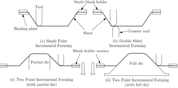
The AISF concept can include different configurations (Jeswiet et al., 2005), as shown Figure 1.1. Its variants allow producing complex sheet components by CNC drive system of a simple tool, with or without the combined use of simple dies. The main common aspect in these variants is the use of a hemispherical forming tool in constant contact with the workpiece. The sheet is also clamped at its edges using a blank holder (Figure 1.1). During forming, the tool travels along the workpiece, following a specific trajectory determined by the user.
3 Figure 1.1: Asymmetric incremental sheet forming variants.
The Single Point Incremental Forming (SPIF) (Figure 1.1.a) variant can be considered as the real dieless forming technology as envisioned by Leszak (1967). The backing plate is used to create an angle transition near the clamped region. Within the AISF process group classification, the SPIF method is also called “negative forming” (Park and Kim, 2003). In SPIF process, the external surface does not contact with any mould or support.
The Two Point Incremental Forming (TPIF), also referred as “positive incremental forming”, was first presented by Matsura in 1993 (Echrif and Hrairi, 2011). Its basic designation is due to the simultaneous contact between two points with both sheet surfaces. The pressure applied between the forming tool and the mould deforms the internal and external surfaces. The TPIF method can be divided in two categories: using a partial die (Figure 1.1.c) or using a full die (Figure 1.1.d) (Attanasio et al., 2008). The partial die (c) is used as a static support to create strength support, influencing the final geometry accuracy. The TPIF with full die (d) uses a mould with the final component shape, located at the opposite surface of the metallic sheet. The mould is normally made using a cheap disposable material, which can be either a negative or a positive die (Reddy and Cao, 2014; Crowson, and Walker, 2015). This technique reduces the springback effect and increases geometrical accuracy (Attanasio et al., 2006 and Callegari et al., 2006). The blank holder device has a vertical displacement through guided columns during the forming process.
The incremental forming with counter tool (see Figure 1.1.b) is named as Double-Sided Incremental Forming (DSIF). It is a variant of TPIF process with an
4
addition of a second forming tool on the opposite surface, independently controlled, instead of a full or partial die. This particularity provides further flexibility to the process and reduces many limitations associated to the remaining variants. Another particularity is the fact that it does not use any backing plate. The main use given to this variant is to the production of highly complex parts (Jeswiet et al., 2005; Malhotra et al., 2012a; Ndip-Agbor et al., 2015).
The purpose of this section was to introduce a brief description on the ISF process variants. A detailed review on technical developments in the last years can be found in the work of Emmens et al. (2010), Nimbalkar et al. (2013), Reddy and Cao (2014) and, recently, by Crowson, and Walker, 2015. In the present work, particular attention is devoted to the Single Point Incremental Forming (SPIF) variant (Figure 1.1.a) and the next section presents a more detailed description concerning this variant.
1.2 Single Point Incremental Sheet Forming (SPIF)
The SPIF concept represents a breakpoint with traditional forming processes. The classic press-stamping process generally deforms the sheet metal in only one stroke (even if multiple steps can occur). The sheet is forced by a punch against a mould, stretching the blank to the desired shape, while the edges are restrained by a blank holder, allowing however some sliding. In the SPIF process, on the other hand, the sheet is gradually deformed by a localized force. In any case, the external surface does not contact with any die or support. The final part is obtained by a toolpath strategy according to the desired final shape. Schematically, Figure 1.2 illustrates the SPIF process setup.
Clamping frame Tool
Backing Plate
Die Sheet
5 The sheet is previously clamped along its edges using a clamping frame (blank holder). A backing plate is necessary to provide an angle change at clamped region and decrease the springback effect during the forming progress. Springback phenomena can also be reduced using a compensatory algorithm (Allwood et al., 2010). The tool is guided through a numerical control system, which defines the toolpath according to the desired final shape. The toolpath can be controlled by using a CAD/CAM software, where a change in the final shape can be fast and inexpensive. The pre-programmed contour combines the continuous contact of the tool along the sheet surface with successive small downward displacements. After each vertical increment, a new contour starts in the next horizontal plane. The component is constructed layer by layer (Figure 1.3.a). However, using a spiral toolpath (Figure 1.3.b) the tool gradually moves down and completes the downward movement equal to the incremental depth every time the tool completes 360º motion along the spiral. Figure 1.3 exhibits different toolpath strategies to perform a conical shape.
Figure 1.3: Contour a) and spiral b) toolpaths.
In general, the main practical setup of the SPIF method consists in the following steps: first, the final product is modelled by a CAD (Computer Aided Design) software, which allows creating a neutral file selected by the user. Next, the neutral file is exported to a CAM (Computer Aided Manufacturing) package. The first step for CAM package is to check the CAD file to visualise potential errors and then the toolpath is created (Jeswiet et al., 2005). Next, the sheet is rigidly fixed on the frame, and the forming tool is controlled with a three-axis CNC
6
(Computer Numerical Control) software machine. Afterwards, during the process, the forming tool is in permanent contact with the sheet surface and moves vertically in each contour. Finally, the spherical tool repeats all these operations until the end of the toolpath, to obtain the final product.
Jeswiet et al. (2005) and (Hirt et al., 2006) summarize the SPIF process advantages and limitations. The advantages are:
the component can be directly formed from the CAD software;
the process can be used in rapid prototyping to produce small number of parts in sheet metal and in polymers;
it does not require expensive tools, i.e., punch and die. However, a backing plate can be necessary to create an angle change near the clamped region;
a conventional CNC milling machine can be adopted for this process; the component sizes are limited to the machine table size;
the operation is quiet and relatively without noise;
the nature of the process involves deformation mechanisms that increase the material formability;
the changes on the component design can be rapidly accommodated changing the CAM file.
The limitations are:
a large forming time compared with the conventional stamping process; process limited to small production batches or prototypes;
it is mandatory the use of multistage forming for steep wall angles, increasing the manufacturing time;
some springback can occur after unclamping the component;
lower geometric accuracy, particularly near the convex radii and bending edges areas.
A number of authors have studied the final product in order to analyse the influence of several parameters involved in the SPIF process. In summary, the following forming parameters are important in SPIF: the geometry of the forming tool, the sheet material, the sheet thickness, the toolpath, the stepdown increment size, the forming speeds (rotation and relative motion) and lubrication (Kim and Park, 2002; Kopac and Kampus, 2005; Cerro et al., 2006; Duflou et al., 2007b; Durante et al., 2009; Ambrogio et al., 2010b). Just a few studies from literature on the SPIF parameters influence are presented below.
7
1.2.1 Forming tool
Typically in SPIF process the tool tip is spherical and ensures a continuous contact point across the metal sheet surface. The relevant variables to the forming tool are its dimension, material and shape. This variable combination affects the time production, the surface quality and the geometry limitation of the final component.
In most applications, the spherical tip is solid and made out of steel. However, to reduce friction and increase tool lifetime can be used other options, such as, surface coating or a free rotating ball tool tip. The application of a polymeric material on the tool tip is used to avoid chemistry reactions or to improve surface quality. There is a wide range of tool diameters, from 4 mm, until a large spherical diameter as 100 mm. The spherical tool diameter values usually are between 4 mm to 15 mm (Jeswiet et al., 2005). Therefore, the optimum tool depends of the product shape, the type of material and the depth at which the spherical tool will work.
The diameter depends also on component dimension and the negative slope (concave shape) of the wall angle. In the wall angle of the component ( ) there is a point from which the tool diameter contact is maximum (Figure 1.4). This instant occurs when the contact point is tangent to the spherical surface. Figure 1.4 illustrates the tangential wall limit with a spherical tool.
Figure 1.4: Wall contact with the forming tool.
To achieve a piece with a steep wall angle, it is necessary to select a forming tool with larger diameter than the sphere body support. The objective is to avoid contact between the sheet wall and the sphere support, as presented in Figure 1.4.A. The body support of the hemispherical head is used to mount the tool on the CNC milling machine shaft. Figure 1.4.B presents a tool configuration used to build a part with a small slope wall. Experiments have demonstrated that smaller diameter tools allow higher metal sheet formability than the use of tools with large diameter (Kim and Park, 2002; Jeswiet et al., 2005; Bhattacharya et al., 2011).
8
Ham and Jeswiet (2006) have studied the influence of the spherical diameter on the maximum wall slope angle. The research work demonstrated a significant increase on the maximum wall angle when tools with smaller diameters are used. The high formability with small diameter tools is a consequence of the force concentration and strains on a small area. The factor restricting the use of a small diameter is the tool resistance under bending fatigue effect.
1.2.2 Material and sheet thickness
The material and the sheet thickness may limit the forming process forces. The forming force involved is the result of the sheet characteristics, its material and its geometry.
Fratini et al. (2004) have investigated the influence of material proprieties on the formability. The tensile test was used for each selected material to determine its parameters. The material parameters were the following ones: strength coefficient (K), strain hardening coefficient1 (n), Lankford coefficient ( r
n), ultimate
tensile strength (UTS) and the elongation percentage (A%). From their SPIF experiments, for each material and using statistical analysis, they determined the influence of the above cited material proprieties. Their analysis concluded that the interaction between the strength coefficient (K) and strain hardening coefficients (n) had the highest influence on formability. Generally, higher hardening coefficients will provide higher formability.
Ham and Jeswiet (2006) have performed a research about the influence of the sheet thickness on the maximum wall angle and showed that increasing the thickness contributes to increase the wall angle. The maximum wall angle defines an indicator of formability. In this work, the interaction between the increasing thickness and the tool size decrease was analysed. The research showed a significant improvement in the wall angle when the tool diameter decreases and the sheet thickness increases.
9
1.2.3 Forming speed
The tool rotation speed and the travel velocity over the sheet surface influence the sliding friction and the frictional heating at the tool/sheet interface. The process time and the final surface quality of the part are the final results which evaluate process performance. The tool relative motion over the sheet is directly proportional to the heat generated by friction. Increasing the speed improves the material formability due to the heating. However, there are negative effects, like higher speed rate, generates higher surface roughness, increases the tool wear and the lubricant film disappears faster. The high rotational velocity increases the probability to develop marks on the sheet surface (Jeswiet et al., 2005; Ambrogio et
al., 2010b; Hamilton and Jeswiet, 2010).
1.2.4 Toolpath and vertical increment
Many experimental studies have been performed to find an optimum toolpath which gives the best results in terms of surface quality. The toolpath and the vertical increment are defined together on the CAM package. These parameters have direct impact on the dimensional accuracy, surface finish, formability, thickness variation and processing time. A number of researchers have discussed their effects and different conclusions were found.
Ham and Jeswiet (2006) have used the forming maximum angle to measure the material formability of AA3003. In their work, they have analysed the influence of the vertical step in the maximum wall angle and it was concluded that there is no significant effect on the final wall angle. Hence, it was shown that the vertical increment has an insignificant influence on the formability.
Many attempts have been performed to analyse various toolpath strategies, such as contour, spiral, radial and multiple-stages. The most common toolpaths are contours or spirals (Figure 1.3) with increasing depth, following the shape profile of the final product.
Attanasio and collaborators (Attanasio et al., 2006; Attanasio et al., 2008) have performed two different toolpaths. In the first experiment the tool followed a series of consecutive contours using a constant vertical step (Z), Figure 1.5.a.
With this strategy, the sheet is marked at the transition point between consecutive toolpath contours. The surface quality is poor when the vertical step has a high value. The second toolpath type tested an experiment with constant “scallop
10
height” (h), Figure 1.5.b. The tool follows a series of consecutive contours with a variable vertical step (Z) in order to keep a constant value of scallop height (h). This strategy avoids the marked transition points and improves the final surface quality.
Figure 1.5: Schematic representation of a) constant vertical incremental (Z) and b) constant scallop height (h).
The vertical step size tends to be related with the wall angle and roughness at the sheet surface. A small step size requires more process time to form the component but the surface quality improves. These experimental tests demonstrated how relevant is the toolpath with a variable step depth (depending on the part geometry). In particular, a correct value of the maximum step depth (Z) and the scallop height (h) must be chosen in order to obtain good results in terms of surface quality, geometric accuracy and thickness of a final component.
1.2.5 Lubrication
The necessity of lubrication is related to the temperature generated at the tool/sheet interface, surface roughness and the forming tool wear (Kopac and Kampus, 2005; Azevedo et al., 2015). The products obtained using the SPIF process are normally functional at its finished shape and, in this sense, the state of the surface is a significant subject. For that reason, the use of lubricants is common.
Kim and Park (2002) have tested two different types of tools, a tool with a free rotation ball at the tool tip and a standard tool with hemispherical tip. Both tools were tested with and without lubrication, which was grease. The authors have observed for the same conditions that the tool with rolling ball on the tip achieves
11 higher formability than the tool with standard tip. Additionally, the results showed that using a standard hemispheric tip without lubrication, it provided occurrence of scratches over the sheet. Finally, using a tool with a free ball on the tip without lubrication was considered the most ideal solution to increase formability. The friction between tool/sheet interfaces increases the tool pressure, lowering the stress state in the sheet. For this reason, damage is delayed and formability increases. A controlled friction at the tool/sheet interface helps to improve the formability. However, if friction increases significantly, it could result in fracture.
1.3 Machinery used in SPIF
Equipment intended for SPIF covers different topologies of machines used in the industry and in academic research. The execution of SPIF process presents essential aspects: it uses a simple spherical tip to build different shapes and the main process feature is the numerical control of the tool axis. The axis control depends of the degrees of freedom (DOF) available on the machine. There are different equipments to produce a component using the SPIF method, such as adopting a CNC milling machine, a robotic arm or a purposely built machine.
The most common applications to perform SPIF experiments has been carried out using an adapted CNC milling machine. Their advantages are the easy upgrade to work as SPIF machine, easily found in industry, considerable stiffness and large productivity rate. On the other hand, it offers a limited number of DOF (Jeswiet et al., 2005). For instance, this choice is the one of Shim and Park (2001), Filice et al. (2002), Jeswiet et al. (2002), Fratini et al. (2004), Ceretti et al. (2004), Ambrogio et al. (2005; 2010a; b), Kopac and Kampus (2005), Araghi et al. (2009), Dejardin et al. (2010), just to mention some research groups.
Similarly, the industrial robotic arm appears as an alternative for many authors, such as Schafer and Schraft, 2005; Duflou et al., 2005; Meier et al., 2005; Lamminen et al., 2005, as summarized by Callegari et al., 2006. They have implemented this solution due to the flexibility given by the available six axes. It allows the tool positioning at different angles relatively to the sheet surface and gives the possibility to combine multiple steps with a single tool. The robotic arm has a large working volume and fast operation. The major drawbacks are the low
12
stiffness and a very low maximum force, which leads to a less accurate tool position, especially under high loading conditions (Jeswiet et al., 2005).
Nowadays, purposely built machines for SPIF process are commercially available, such as the one developed by the Amino Corporation (Amino et al. 2002). However, a number of academic research groups have developed their own machine to perform the SPIF process. As examples, the machine from Julian Allwood’s group at University of Cambridge (Allwood et al. 2005) and the innovative prototype machine called SPIF-A at University of Aveiro (Alves de Sousa et al., 2014). This last referred SPIF machine introduced a Stewart platform (Yau, 2001) adaptation, allowing six independent degrees of freedom. Figure 1.6 exhibits the innovative prototype machine developed at University of Aveiro based on Stewart platform purposely adopted for SPIF.
Figure 1.6: Prototype machine for SPIF from University of Aveiro.
Among these different equipment options, the use of CAD/CAM software is the common feature between them to obtain a toolpath. The CAD model of a component is converted into a neutral file (STL) containing the geometric information. Afterward, the CAD model is sliced into horizontal layers through the CAM software and converted into a toolpath. Figure 1.7 exhibits the standard strategy to build a toolpath.
13 Figure 1.7: Standard strategy to build a toolpath for SPIF.
A brief overview of the SPIF process has been given based on the available literature. In this context, previous sections introduced a general understanding of SPIF process which will be the focus of the present work study. Section 1.4 presents the thesis scope and motivation, while Section 1.5 summarizes its contents.
1.4 Motivation and Scope
Many issues appear when simulating the SPIF process by the Finite Element Method (FEM). As always, a compromise between accuracy and CPU efficiency is necessary. Accuracy from the results of numerical simulations, specially related to the prediction of the forming forces, is important since it contributes to the protection of the tool and the machinery used in the process.
The present work aims to give a relevant contribution to the state-of-the-art and knowledge level of the SPIF process, from both academic and industrial standpoints, thus increasing the process feasibility in the numerical simulation field. In this topic, since the tool/sheet contact status changes continuously and only a small area is plastically deformed at each time increment, common methodologies resorting Finite Element Method (FEM) codes lose efficiency. The time increments become small and consequently the simulations take huge CPU time.
The work will focus on the numerical simulation performance based on the FEM, in order to reduce the high computational time of SPIF simulation. The main task includes the implementation of the Finite Element technology, with new elements such as those related to solid-shell finite element formulations and
14
remeshing algorithms. Solid-shell finite elements allow the automatic consideration of thickness variations taking into account 3D stress analysis. The use of different constitutive laws cover applications with distinct materials, such as aluminium and steel alloys, to assess the numerical accuracy.
An improved numerical simulation within the SPIF framework combined with accurate material modelling can be seen as the final objective. Benchmark proposals are used as case-studies to evaluate the numerical simulation predictions compared with experimental measurements.
1.5 Main objectives
The framework of this thesis is the numerical simulation of asymmetric and axisymmetric component shapes incrementally made using SPIF process based on FEM supported by experimental validation. The numerical simulations include the adaptive remeshing method combined with a hexahedral finite element, more properly the use of the RESS (Reduced Enhanced Solid-Shell). More details on this solid-shell element can be found in the series of works from Alves de Sousa et al. (2005; 2006; 2007). The choice of a solid-shell formulation to simulate sheet metal forming operations is also based on the possibility to use a general 3D constitutive law behaviour, while classical shell finite elements are implicitly based on plane stress/strain assumptions. Additionally, thickness variations and double-sided contact conditions are easily and automatically considered with solid-shell finite elements.
The main goals aim the implementation of the RESS finite element, especially designed for sheet metal forming, in the in-house FEM code named LAGAMINE (Cescotto and Grober, 1985). The extension of the adaptive remeshing technique, currently available in LAGAMINE code for a shell element (Lequesne et al., 2008), to use it with the mentioned solid-shell element. These features are not available in common commercial FEM codes. Implicit analysis is used to perform the numerical simulations. It is worth noting that no previous work has been carried out using remeshing strategies with hexahedral elements on SPIF, which makes this work innovative.