Abstract: This paper presents a regulation mechanism aiming to position agricultural tools relatively to the previous lines, while sowing or harvesting. The sowing rows were revealed by a background correction, the background being obtained thanks to a median rank filter. The method was found efficient in eliminating the shadows. For the crop rows (chicory rows), a neural network was used to localise the plants. While the petiole and the leaves were easily separated from the soil, the chicory root and the soil having about the same colour and the lighting condition varying widely, it was more difficult to obtain a good contrast between those parts, which leaves place for some improvements. The adapted Hough transform consisted in computing one transform for each line in the cluster with, for reference, the position and direction of the theoretical position of the row. The different transforms were then added. The position was used in a feedback regulation loop. An articulated mechanism was used to ensure the lateral displacement of the tool relatively to the tractor. The behaviour of the whole outfit was studied during several field tests. The standard deviation of the error, measured as the difference between the observed inter-row distance and its theoretical value, was of 23 mm for sowing and 31 mm for harvesting and its amplitude was less than 100 mm for sowing and less than 115 mm during the harvest, which was sufficient to fulfil the requirements of the application. Sources of systematic errors were also identified as linked to the geometric considerations. Their correction requires an accurate mounting of the camera, which may be possible for a serial montage.
Keywords: automatic guidance, Hough transform, line cluster, seed drill, crop rows.
I. INTRODUCTION
The lateral position of agricultural tools, such as seed drill relatively to a previous passage or harvesting machines relatively to crop rows, are usually controlled by the driver of the tractor. The precision of the drilling determines the feasibility or not of subsequent works like mechanical weeding or harvesting with machines having a width not matching the seeding width (in term of line number). For example, most sugarbeet seed drills in Belgium are of twelve rows width while the harvesters are of six rows. Some machine builders however marked an interest for eight row harvesters, to enhance the harvesting performances. Though an experienced driver may actually be able to achieve the required driving accuracy, which requires to maintain the
amplitude of lateral movements of the drill below 150 mm around the nominal value (usually 450 mm), this task needs some concentration and could hardly be maintained during a long period, especially pointing out that the supervision of the drill itself also needs a part of the driver's attention. Under these circumstances, a driving assistance would be welcome.
The problem of guiding automatically a tool in a field using machine vision is not new. This literature review is limited to papers concerning prototypes used for field agricultural applications. Recent researches could be divided into the conception of either autonomous steering or guidance assistance. The techniques were used to evaluate the position of the tool in the field relatively to the culture rows or to the edge of the harvested part of the field.
Billingsley and Schoenfisch (1997, [1]) presented a method to steer a tractor by following culture rows such as cotton, for which the row may not appear continuous in the images, depending on the stage of growth. In order to localise crop rows the pixels were segmented between ‘plant’ and the surrounding by thresholding, the value of the threshold being determined by the proportion of plants. The lines were localised by regression, the offset and the slope parameters being used as state variables.
Hague et al. (2000, [2]) presented an experimental autonomous vehicle guided by a machine vision system and additional sensors (odometers & inertial sensors). A Hough transform was used to localise the row structure and an extended Kalman filter ensured the fusion of the different sensors information and to obtain the position of the vehicle.
Tillett and Hague (1999, [6]) and Tillett et al. (2002, [7]) developed a hoeing system for weed control in sugar beet. The camera was mounted on a hoe attached to the tractor three-point linkage through a mechanism allowing a lateral displacement. The camera was a mono-chrome charge-coupled device (CCD) equipped with a near infra-red band-pass filter. The lateral displacements were ensured by two hydraulic cylinders and the hydraulic flow was controlled by a three states valve. A linear variable differential transformer gave the lateral position of the hoe. In Tillett et al. (2002, [7]), the image was divided into height horizontal bands, each merged vertically to give horizontal profiles. The position of the crop rows were found by matching a template profile. The extended Kalman filter was used to track the hoe position. The measurements were the position in each band and the state vector had three elements: the lateral position, the heading angle and a correction for the camera misalignment. During the computation of the recursive filter, the error between the measured and the expected position was
Agricultural tools guidance assistance by using machine vision
Leemans V., Destain M.-F.
Faculté des Sciences agronomiques de Gembloux – Unité de mécanique et construction Passage des Déportés, 2 – B 5030 Gembloux, Belgium
evaluated. If this value was too big, the data were ignored, otherwise they were incorporated in the state estimation. The trueness was below 10 mm, while the precision was within 16 mm.
Pilarski et al. (2002, [4]) presented an automated
self-propelled win
drower with a regulation based on a camera or on a differential global positioning system (DGPS) associated with other sensors (inertial & wheel encoder). These systems were tested independently to harvest a field autonomously, after the ‘opening up’ by a human operator. The edges of the cut and un-cut areas were localised using the difference in reflectance, after a compensation of the shadows. Authors also detected the end of crop row (where there was no more edge) and obstacles (based on their different colour). The system could work at 1.5 to 2.0 m/s. The vision based error was in range of 50 to 300 mm, while the error of the DGPS was in a range from 40 to 60 mm.Søgaard and Olsen (2003, [5]) mounted a camera on a hand operated vehicle and later on a weeder to evaluate the precision of an algorithm based on image analysis. The images were also divided into band strip which were mathematically ‘enrolled’. The centre of gravity gave the position and an estimation of the relative accuracy. A weighted linear regression gave the position of the rows. The mean position returned by their algorithm (trueness) was centred. The standard deviation (precision) was about 15 mm. The working speed was of 0.4 m/s. These results however concerned the image analysis, not the position of a tool.
The aim of this work was similar to row tracking but there is a main difference: the detection was based on images where a target (the seed lines), being of the same nature as its surrounding, was feebly contrasted. This paper aims to show that the signals issued from that process are valuable to control the lateral seed drill movements.
II. MATERIALANDMETHOD A. The hardware
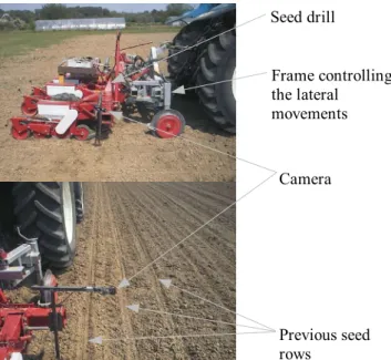
The field experiments were carried out using a device allowing a lateral movement between the drill and the tractor, as shown in Fig. 1. The device was a piece of a mechanically guided hoe (from Agronomic, France) composed of two frames, attached respectively to the tractor and to the tool and joined by two links. The lateral movements were produced by two cylinders, controlled by a three ways ‘right on – off – left on’ distributor, itself droved by a laptop computer, using its parallel interface. A joystick could also be used by the operator for manual control. For the harvesting, the camera was placed below the moving frame in such a way that it observed two rows between the rear wheels of the tractor. For the sowing experiment, a precision seed drill (“Précis +”, six rows, Gilles S.A., Belgium) was coupled to the device. The relative position of the seed drill compared to the previous lines was recorded thanks to a camera fixed to the drill (Fig. 1), allowing the two lines to be visible in the images. The camera was a Unibrain Fire-iA400 1394 (Unibrain S.A., Greece) equipped with a lens having a focal of 6 mm. It was a colour mono-CCD camera. The automatic settings of the electronic shutter were found suitable for the application. This device was controlled by the computer through the IEEE 1394 port, thanks to the ‘1394 Digital Camera Driver’ (The Robotic Institute, Carnegie Mellon University, PA , USA). The management of the videos and of the images, the image filtering were made by using the Open Source Computer Vision Library (Intel Corp.). The codes of the adapted Hough transform and the post filtering were written in C++.
B. The algorithms
The regulation of the seed drill in position corresponds to the general block diagram presented in Fig. 2. The true position was evaluated by using image acquisition, pretreatment and analysis (the measurement). This process suffered from noise (the measurement noise) and the signal issued from the image analysis was therefore treated before being used. The estimated position was then compared with the reference. The error dx was transformed into a pulse driving the opening of the distributor (the pulse width was
Figure 1 : Experimental set up used for the field tests. The seed drill was coupled to a frame allowing lateral movements relatively to the tractor, which pull the whole. The camera was used to record the position of the drill relatively to the previous seed lines.
Frame controlling the lateral movements Seed drill Camera Previous seed rows Regulation Process Measurement Signal treatment dx
movement to the left or to the right, dt Target position + -Process noise True position Measurement noise xb,
r
k
m rm
related to the amplitude of dx, the sign of the error determining the direction of the movement) and the translation device converted it into a displacement of the seed drill (process). The new position resulted from the addition to the previous position, of this displacement and of the lateral and angular movements from the tractor, which constituted the process noise.
Detection of sowing rows
The camera was requested to send 640 by 480 pixels RGB colour images, with a frame rate of 15 images per second. The integration time, the brightness and the gain were adjusted automatically by the camera. The green channel was used and the image size was reduced to 106*80 pixels.
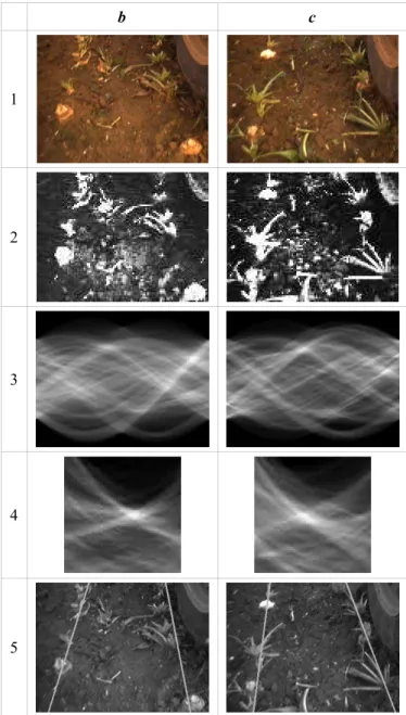
The bases of the image treatment are presented in Fig. 3. The sowing lines appeared as dark thin lines on a brighter background, but the ‘noise’ was important relatively to the relevant information. The image treatment consisted in a Gaussian filtering (3 × 11 pixels) and a background subtraction to remove the shadows. The background was computed using a wide median filter (5 × 5 pixels) which preserved the boundaries of the large areas of the image while removing the narrow linear elements. Subtracting the image from the background gave an image with the sowing lines appearing as bright lines on a dark background.
Detection of chicory rows during harvesting
These tests were carried out after a passage of the leaf stripping (machine placed at the front of the tractor) and before the harvesting (the harvest shares are placed behind the tractor). The scene presented in Fig. 4 shows, apart from the soil (brown), parts of the machine (red wheel rim and dark tyre), chicory roots (light brown, more orange than the soil), petioles (green), root flesh (whitish). Occasionally parts of leaves ripped off the roots were thrown between the rows. Chicories outside the rows or weeds were also encountered in some places. All the chicory parts were not visible on each image and only a few plants were missing. The lighting condition could be sunny to cloudy which means that the images could show sun and shadow areas or a more or less homogeneous illumination.
To reveal the plant rows with such a variability, a neural network was used to detect pixels belonging to the ground from those belonging to a chicory. Orientation experiments were carried out to determine its structure : a two layer perceptron with one hidden layer. A set of five parameters were used (R, G, B and the means for R and B) to feed the neural network. Three neurons were necessary in the hidden layer. The computation of the means was based on a systematic sub-sampling of the image (one pixel out of twenty-five). Sigmoidal transfer functions were used for both layers of the perceptron.
The training of the neural network was carried out “in-line” (using FANN, fast artificial neural network library, Steffen Nissen, U.K.) During that phase, the tools had to be positioned accurately by the driver.
The images were resized to the third of their original size (106 pixels wide and 80 pixels high). After having computed the required statistics on the image, the data of each pixel were fed into the neural network which returned values between 0 and 1. For control purpose, these values were
a b 1 2 3 4 5 6 7
Figure 3 : Pretreatments of the sowing row images. 1 : Original images. 2 : Images after resizing and Gaussian filter. 3 : Background images (after median filter). 4 : Images after background subtraction. 5 : Results of the classical Hough transform. 6 : Results of the adapted Hough transform. The grey scale of the images on row 5 and 6 were adjusted so that the minima were represented in black and the maxima in white. 7 : Results of the detection on the original images.
multiplied by 255 and displayed as presented in the second row of Fig. 4. The plant rows appear in bright while the ground and the machine remain darker.
Adaptation of the Hough transform for cluster lines detection
The detection was performed using a modified Hough transform. The Hough transform was designed to detect curves in images, amongst other straight lines. Though chicory rows do not appear as continuous lines, the alignment of plants could also be detected with this method.
The basic idea was to perform one transform for each line with a specific reference point corresponding to each line in the cluster. The results of this treatment were the Hough
space coordinates computed for the right rows, relatively to its nominal position (when the drill is correctly positioned).
As stated amongst others by van der Heijden [10], a straight line can be represented as an equation of the angle α of the line with a reference direction and of the distance r to a reference point, according to Fig. 5 (left) :
x−xrefcos− y− yrefsin −r=0
with ∈[0,] , r∈ℝ (1)
The reference point is usually the centre of the image and the reference direction the horizontal. A line in the (x,y) plane is thus represented as a point in the (α, r) plane (the Hough space – Fig. 5). A bright line on a dark background appears as a maximum on the transformed image (Fig. 3, line 5, Fig. 4, line 3).
When the camera observed the crop rows, several ones were visible in the image as shown in Figs 3 and 4. On the ground, the culture rows are parallel with a given spacing and appeared in the images as almost straight and sequent lines. The spacing and orientation of these lines in the image depend on the geometry of the image acquisition (focal length, CCD dimensions, tilt of the camera). We made the assumption that all those lines converged to the same point (out of the image, Fig. 5) and that the angle and the distance between these lines remained constant when the machine (and thus the camera) offset or changed its direction relatively to the previous sowing traces or to the plant rows. The angles and distances were thus related by the following equations : xi− j= −ri cosi rj cosj (2) i− j=i−j (3)
When the camera moved with reference to the culture row, the lines in the images and their corresponding maxima in the Hough transform image also moved, but their relative positions remained unaffected.
In order to detect the cluster of lines in one operation, one transform was carried out for each line, but with different angular and lateral references, so that the maximum representing each line was positioned at the same point of the Hough space, as shown right in Fig. 5. The Hough transform was then given by :
x−xref icos−i− y− yrefsin −i−r=0
with ∈[−/2,/2] , r∈ℝ (4)
The reference points were chosen at the intersection of the horizontal median of the image and the considered (the ith) reference lines (yref was thus constant). The reference angle was the one of the perpendicular to the considered reference line (Fig. 5, right). The number of reference lines, points and angles were equal to the number of rows in the line cluster.
The values of each part of the transform were summed. The maxima corresponding to the culture row were added, while others peaks resulting for example from the tillage, ripped leaves or weeds were added to the noise and thus diluted. When the sowing machine was correctly positioned, the coordinate of the maxima should be in (0,0).
b c 1 2 3 4 5
Figure 4 : Results of the Hough transform applied to the detection of a cluster of lines – localisation of chicory rows. 1 : Original image; 2 : Images treated by neural networks; 3 : Results of the classical Hough transform; 4 : Results of the adapted Hough transform. The grey scale of the images on row 3 and 4 were adjusted so that the minima were represented in black and the maxima in white; 5 : Results of the detection on the original images.
The signal treatment
The estimated Hough space coordinates αe and re were used
as state variables. The position of the right line at the top (xa)
and the bottom (xb) of the image were given by: xa=l 2 re cose −h 2 cose
(5)
xb= l 2 re cose h 2 cose(6)
where: h is the image height and l the image width. This latter was used as the estimated position of the drill. The parameters αe and re were estimated independently (at step k),
using their measures in the image αm and rm, their previous
estimations (at step k-1) and the deport caused by the regulation drr:
e re
k =
a 0 0 ar
m rm
k
1−a 0 0 1−ar
e re
k−1
0 drr
k−1(7)
a=cexp
−[ek−1−m] 2 s2
(8)
ar=crexp
−[redrrk−1−rm] 2 sr 2
(9)
cα, s2α, cr and s2r were parameters adjusted on measurement
made on videos acquired in field (Leemans & Destain, 2006, [3]). The earlier version of the algorithm used on that occasion showed that the measurement noise was not of
Gaussian type but rather constituted by several noises and this non linear recursive filter was then found useful. As it is obvious that α has an influence on r, laboratory tests were made to check the interest to incorporate the angle between the tractor and the rows in the estimation of the position. This was found effective but this required an accurate orientation of the camera. This latter was deported compared with the drill and for this reason, during the field experiments, it was removed for the transport between the laboratory and the field. During the mounting of the camera in the field it was found difficult to adjust precisely the orientation of the camera (the main problem was to ensure that the drill was quite perpendicularly to the previous lines). The lateral movement of the seed drill would also result in a change in the apparent angle of the row in the trace. However, as the lateral displacements were limited by the regulation itself, this was not considered.
The regulation and the process
The lateral displacement of the tool relatively to the tractor was controlled by adjusting a pulse width, conditioning the opening time of the distributor at each time step. The relation between the pulse width and the lateral displacement was analysed and below 200 msec (which is far more than the interval between two images), a linear relationship between the lateral speed v and the pulse width dt was found. The opening time for a given error dx was thus given by:
v= p dtq
(10)
v=dx /dt(11)
p dtr 2 q dtr−dx=0(12)
(0,0) α r α r 0 1 2 x y + + + θ12 . . . , + : theoretical position , . : true position 0 1 2 Reference point : projection line : integration directionClassical Hough transform
The « Hough space »
(0,0) α r 0 1 2 x y θ12 0 1 2 α r + ... α r + . .. , + : theoretical position , . : true position Reference point : projection line Reference direction
The « Hough space »
Figure 5 : Principle of the Hough transform adapted to the detection of a line cluster. The classical transform is illustrated left and the adapted one right.
dtr'
dtr' '=−
q±
q2 4 p dx2 p
(13)
where p and q are the linear regression coefficients and the negative root dt'' having no meaning. The small errors, in range of ± 13.3 mm, were not corrected.
Laboratory tests were also carried out to fit the values of p and q and to estimate the cutting frequencies of the different part of the regulation. These showed that the cutting frequency of the process (hydraulic & mechanical devices), acting as a low pass filter, was above 0.3 Hz. The cutting frequency of the signal treatment, the regulation and the process was evaluated at around 0.22 Hz.
C. The field experiments
The seed drill field tests were carried out just after the sowing period in order to dispose of the seed drill at leisure. Each test consisted in a first passage of the drill, with the guiding assistance system turned off. On the second passage, the driver followed the usual guide while the guiding system corrected the relative position of the drill. In order to solicit the device at higher frequencies, for two of the tests the driver was instructed to follow a sinusoidal trajectory, relatively to the previous line. Horizontal blue marks were placed in the field of view of the camera in order to synchronize the field measurements and the data recorded by the programs.
During each test, the program recorded several parameters and a video. These data were used to get the measurement noise.
After each test the distance between the last seed line of the previous passage and the first seed line of the controlled passage was measured with an sampling interval of 0.5 meter. This will be hereafter called the position of the seed drill. One of the seeding elements was lifted and a plough coulter was fixed at its place on the fix frame attached to the
tractor. The distance between the trace left by this coulter and the last seed line was also measured and was considered as the measure of the lateral displacement of the tractor (here after named position of the tractor).
During the experiments the weather was sunny. Only during one day of tests there were some clouds and one test was carried out in diffuse lighting condition (test 5).
The harvesting field tests were carried out in a similar way, except that the reference was the culture row.
III. RESULTS
The tractor speed varied from 0.91 to 0.95 metre per seconds. The image acquisition frequency varied from 9.9 to 10.2 images per second when a video was recorded (otherwise, the 15 images per second delivered by the camera can be processed). These data were considered to be sufficiently constant to have no effect on the behaviour of the regulation.
A. Detection of sowing rows
The results of the pretreatments are shown in Fig. 3. Most of the shadows were removed by the background subtraction. Only a thin part of the shadow of the tractor's door remained (the thin oblique line). This had no consequence, because the orientation of the line drawn by that element on the image had a direction which could not be confused with the researched objects. This also means that vertically elongated objects should be avoided near the camera, because they could produce shadows like the sowing lines. The contrast which, on the original image was less important in the shaded part, remained smaller in those parts of the pretreated image. Nevertheless, the lines were visible in that part too. The seed lines often appeared as thin double lines (a central hollow and a shadow of one border). One of these was detected by the algorithm which could produce a slight bias.
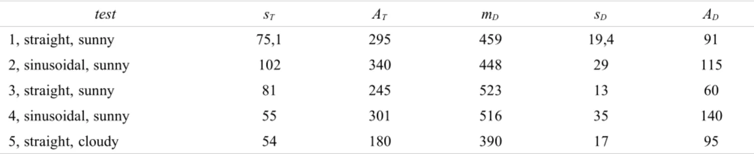
Table 1: Main results of the five field tests with the drill. sxb is the standard deviation of the position xb (computed for the
whole test); sxb and msxb were evaluated from within the images; sT is the standard deviation of the tractor’s position; AT is
the amplitude of the tractor’s position; mD is the the drill’s mean position; sD is the standard deviation of the drill’s position; AD is the amplitude of the drill’s position
test sT AT mD sD AD 1, straight, sunny 75,1 295 459 19,4 91 2, sinusoidal, sunny 102 340 448 29 115 3, straight, sunny 81 245 523 13 60 4, sinusoidal, sunny 55 301 516 35 140 5, straight, cloudy 54 180 390 17 95
Table 2: Main results of the five field tests during the harvest. sxb is the standard deviation of the position xb (computed for
the whole test); sxb and msxb were evaluated from within the images; sT is the standard deviation of the tractor’s position; AT
is the amplitude of the tractor’s position; sD is the standard deviation of the drill’s position; AD is the amplitude of the drill’s
position
test sT AT sD AD
1, straight, cloudy 19 65 17 55
B. Detection of chicory rows
The ratio of pixels correctly classified was around 70% (this is for the validation data, the learning and stop set presented usually a higher rate, around 80%). The first row of Fig. 4 shows the results.
C. Deviation from the reference
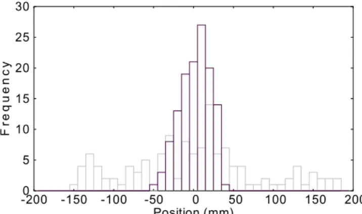
The main results are summarised in Table 1 and 2. The field measurements are presented in detail under different graphical forms for the first test of the seed drill regulation : Fig. 6 plots the position of the tractor and of the seed-drill against the covered distance; Fig. 7 shows the histograms of the positions while Fig. 8 shows the frequency decomposition of the tractor's movements and of the drill movements. For a better readability of the graphs in Fig. 6 and 7 the data were centred. A detrend process was applied to the data before the Fourier transforms in Fig. 8.
During the first test the instruction to the driver (who was not a trained driver) was to follow the previous lines. It is obvious that the observed trajectory was not parallel to the previous one but deviated and that the driver corrected twice at around 20 metre and at around 40 metre. However, apart from these corrections, the trajectory was rather straight.
The mean position of the seed drill (trueness, mD Table 1) depends on the mounting of the camera. For the first two
experiments, this was done carefully and the values were close to the theoretical width of 450 mm. For the other tests the mounting was done more approximately (because it required time) and the values were less precise. This does however not seems to be a real problem in the eventuality of an industrial application. There was another origin for a difference between the target value (450 mm) and the measurements. The border of the trace left by the drill was sometimes more visible than the central hollow, as it can be observed in Fig. 1. In this case the mean position can deviate by 20 to 30 mm.
The reduction in the amplitudes of the movements of the drill compared with the amplitude of the tractor's movements can be seen in Figs. 6 and 7 as well as in Table 1. The dispersion of the drill's position was symmetrical around the mean and appeared bell-shaped (Fig. 7) while the distribution of the tractor's position was more flat : the standard deviation of the positions dropped from 73 mm for the tractor (mean value of sT, Table 1) to 23 mm for the drill while the corresponding value for the amplitudes lessened from 272 mm to 100 mm. As the harvesting machines which would eventually harvest the crop can tolerate up to 150 mm misalignments between rows sowed by different passages, the values of the trueness, of the precision and of the amplitude are well beyond this tolerance and are thus totally compatible with this application. For applications such as mechanical weeding, better performances should however be achieved. Tests 1, 3 and 5, for which the driver was instructed to drive “straight”, showed lower values of dispersion than tests 2 and 4 for which the driving was of sinusoidal type (standard deviation and amplitude below the corresponding means for the first group, above for the second). The same observations are also valid for the harvest test. The lighting conditions were not found to have any effect neither on the trueness, nor on the precision.
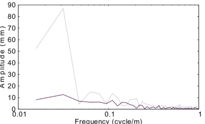
The causes of dispersion of the position of the drill was linked to the lack of ability of the system to correct the movements of the tractor and to the noise added during the measurement and the process. The cutting frequency of the mechanical and hydraulic part was close to 0.3 Hz (the corresponding spatial frequency should have been slightly above 0.3 cycle/m). The diagrams in Fig. 8 show that around and above that frequency the tractor movements were quite small and the mechanical filtering fortunately did not play a significant role in the regulation. The same diagrams show that the amplitudes of the drill movements were quite smaller than those of the tractor's movements, especially for the low frequencies. The cutting frequency, evaluated as the frequency showing an amplitude ratio of -3dB, was of 0.14 cycle per meter, corresponding to a wavelength of 7 m. This spatial frequency was slightly lower than the evaluation made in the laboratory. However, for a “normal” driving style, the amplitudes at these wavelengths were already low (Fig. 8). This corroborates the observations made from Table 1 and 2 : when the driver adopted a 'soft' driving style, the regulation was able to operate more accurately than in the case of rapid direction changes.
The evolution of the parameters recorded during the tests showed that the apparent movements of the traces in the image seemed feeble, exceeding the theoretical limit (± 13.3 mm) only slightly. The standard deviation of the
-200 -150 -100 -50 0 50 100 150 200 0 10 20 30 40 50 60 70 P o s it io n s ( m m ) Covered Distance (m)
Figure 6 : Position of the tractor and of the seed-drill relatively to the previous seed row, against the covered distance. Test 1, centred data. In grey: the position of the tractor; in black: the position of the actual seed row
0 5 10 15 20 25 30 -200 -150 -100 -50 0 50 100 150 200 F re q u e n c y Position (mm)
Figure 7 : Histograms of the position of the tractor and of the seed-drill relatively to the previous seed row, against the covered distance. Test 1, centred data. In grey: the position of the tractor; in black: the position of the actual seed row
measurement noise of the displacement of the trace in the image was systematically lesser than the corresponding measure on the ground. The noise resulting from the images analysis was conform to the previous studies (Leemans & Destain, 2006, [3]) showing similar values of precision (22 mm, before filtering). Its low frequency content had low amplitudes, with peak around 5 to 8 mm (unshown), relatively smaller than those of the drill (Fig. 8). This means that other errors sources had to be considered.
Beside the measurement noise, other errors in the estimation of the position were observed. Two geometrical systematic errors were identified. The first one was linked to the angle of the tool relatively to the previous line. The position was estimated at the bottom of the image but the traces left by the seeding element were made 1.5 meter backward (as it can be seen Fig. 1, above). The correction of this error could be quite straight forward though the angle must be estimated correctly, which requires a correct alignment of the camera. A misaligment of 0.015 radian (0.85°) would thus produce an error in the range of the standard deviation of the position. Tillet et al. (2002) overcame this problem by adding it as a third state variable (with the lateral position and the angle). Another aberration came from the difference of curvature between the previous row and the actual trajectory. This would be more complex to deal with, as the curvature could not be evaluated within an image, the portion of rows observed being too short. The difference in curvature should be inferred from the changes in the angle between previous and actual values of α or from the steering angle of the tractor’s steering wheels. As explained above, an accurate evaluation of this angle could be used to enhance the prediction of re and increase the cutting
frequency. Because of their origin, these two errors are linked to the state variables re and αe and have similar
spectral distributions. They could thus not be filtered. IV. CONCLUSIONS
The performances of a guidance assistance mechanism was analysed during field tests by measuring the difference between the observed inter-row distance and its nominal value (450 mm). The trueness of the system (the mean of the difference) was strongly influenced by the mounting of the
camera. When this later was mounted properly, the trueness was below 30 mm, due mainly to the aspect of the trace left by the drill. For the seed drill tests, the precision (the standard deviation) was of 23 mm and the amplitude of 100 mm, while the corresponding values for the tractor were of 73 mm and 272 mm respectively. For the harvesting test, the standard deviation dropped from 43 mm for the tractor to 31 mm for the tool and the amplitude from 160 mm to 115 mm. These values would ensure the compatibility of seed drill having a guidance assistance with non matching width harvesting machine. During the field tests, the driver was asked to drive normally for some tests and to drive sinusoidally for the others. The value of precision and amplitude of the former driving style were lower than those of the latter. This means that rapid direction changes should be avoided, in profit of a smoother driving style.
A detailed analyse of the results showed that the whole system acted as a low pass filter having a cutting spatial frequency of 0.14 m-1. Apart from the measurement noise, two other errors sources were identified. The first one was linked to the distance between the estimated position of the drill (at the bottom of the image) and the actual position and the second to the difference of curvature between the previous row and the actual trajectory. The correction of the first error as well as the increase of the cutting frequency could be achieved by better taking into account the orientation of trace in the image. This imposes an accurate mounting of the camera, which was not possible in the context of these experiments, but could be achieved for an industrial application.
V. ACKNOWLEDGEMENTS
This research was funded by the Walloon Region (Direction Générale de la Technologie et de la Recherche), convention FIRST SPIN off, 011/4797.
VI. REFERENCES
[1] Billingsley, J., Schoenfisch, M., 1997. The successful development of a vision guidance system for agriculture. Computers and Electronics in Agriculture, 16, 147-163. [2] Hague, T., Marchant, J.A., Tillett, N.D., 2000. Ground
based sensing systems for autonomous agricultural vehicles. Computers and Electronics in Agriculture, 25, 11-18.
[3] Leemans, V., Destain, M.-F., 2006. Line cluster detection using a variant of the Hough transform for culture row localisation. Image and Vision Computing, Accepted. 4] Pilarski, T., Happold, M., Pangels, H., Ollis, M.,
Fitzpatrick, K., Stentz, A., 2002. The Demeter system for automated harvesting. Autonomous Robots, 13, pp. 9-20. [5] Søgaard, H.T., Olsen, H.J., 2003. Determination of crop
rows by image analysis without segmentation. Computers and Electronics in Agriculture, 38, 141-158. [6] Tillett, N.D., Hague, T., 1999. Computer-vision based
hoe guidance for cereals – an initial trial. Journal of Agricultural Engineering Research 74, pp. 225-236. [7] Tillett, N.D., Hague, T., Miles, S.J., 2002. Inter-row
vision guidance for mechanical weed control in sugar beet. Computers and Electronics in Agriculture, 33, 163-177. 0 10 20 30 40 50 60 70 80 90 0.01 0.1 1 A m p lit u d e ( m m ) Frequency (cycle/m)
Figure 8 : Frequency analysis of the movements of the tractor and of the seed-drill, Test 1. In grey, amplitudes of the tractor displacements; In black, amplitudes of the seed-drill displacements.