ALE Methods for Determining Stationary Solutions Metal Forming Processes

ALE METHODS FOR DETERMINING STATIONARY

SOLUTIONS OF METAL FORMING PROCESSES

R. Boman⋆† _{and J.-P. Ponthot}⋆

⋆_{LTAS-MC&T – Continuum Mechanics and Thermomechanics, University of Li`ege,}

1, chemin des Chevreuils, B4000 Li`ege 1, Belgium, voice: 32 4 366.93.10, fax: 32 4 366.91.41, e.mail: [email protected], [email protected],

web page: http://www.ulg.ac.be/ltas-mct/

† _{Boursier FRIA}

Key words: ALE Methods, Convection, Stationary solutions, Rolling.

Abstract. In this paper, two efficient convection algorithms are briefly presented in order to update the values stored at the Gauss point during the Eulerian step of an Arbitrary Lagrangian Eulerian computation in solid mechanics. They are based on the finite volume method and on the Streamline Upwind Petrov Galerkin method. Two applications are presented : a cold rolling simulation and a drawbead simulation.

1 INTRODUCTION

The general frame of this paper is in the field of numerical simulation of forming pro-cesses by the finite element method. In order to find the solution of steady state propro-cesses by numerical simulation with the classical Lagrangian formulation, very large and use-less meshes have to be considered. For example, when dealing with rolling simulation, a large part of the sheet has to be discretised even if the results in the first finite elements, which are introduced between the rolls, are not important. However, these finite elements cannot be removed because they are required in order to reach the steady state solution. Consequently, the CPU time is very large. Another approach is the well-known Eule-rian formulation: the media flows through the mesh, which is fixed in space. However, boundary conditions are rather difficult to handle particularly frictional contact and free surfaces.

The Arbitrary Lagrangian Eulerian (ALE) formulation was introduced to overcome these problems (see e.g. [7, 8, 2] ). The mesh can be handled by the software, irrespective to the body motion, so that both previous formulations can be obtained as particular cases if the mesh sticks to the body or is fixed in space. In such a formulation, time steps are divided into two phases: the first one is Lagrangian and the second one a convective Eulerian phase, where the values stored at the Gauss points have to be updated. In order to avoid oscillations and instability, efficient convection algorithms have to be used. In the present paper, two convection methods will be presented and compared: the first one, called ‘Godunov-type update technique , is based on a finite volume method and the second is based on the Streamline Upwind Petrov Galerkin (SUPG) method. This work has been introduced in MEFAFOR [7], the non-linear finite element code developed at the LTAS, University of Li`ege, Belgium.

2 THE GODUNOV-TYPE UPDATE TECHNIQUE

Once the first (Lagrangian) step is completed, the studied body is automatically remeshed by the program following the users instructions (it can be a minimization of the meshs distortion or, in the case of stationary processes, most of the nodes are fixed in space). When non linear problems are considered, some important values, like the stress tensor or the equivalent plastic strain, are stored at the Gauss points and have to be updated from the Lagrangian mesh to the new one. This convective step consists of solving a classical convection equation, which can be written :

∂ σ

∂ t|χ+ wj ∂ σ ∂ xj

= 0 (1)

where σ is a value stored at the Gauss point (e.g. a component of the stress tensor), wj is the relative velocity between the new mesh and the Lagrangian mesh and χ is the

Although this scalar equation is well-known in fluid mechanics, it is rather difficult to solve it because σ is not a continuous field but is only defined at the Gauss point. Consequently, the gradient cannot be evaluated.

In order to overcome this problem, the values can be extrapolated and averaged to the mesh nodes and the gradient is computed from the resulting continuous field. But this first simple method shows a large amount of numerical diffusion. More sophisticated methods must be used.

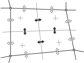
Figure 1: A finite element and its division in 4 finite volumes

The Godunov-update technique was firstly introduced by Casadei, Don´ea and Huerta [4, 5]. This method can be useful on structured meshes of Q4P0 hybrid finite elements (4 Gauss points are used to integrate all the values except pressure, for which 1 point is used to prevent locking). It consists of dividing each finite element into four (one for the pressure) cells surrounding each Gauss point (fig. 1). The field to be transferred is assumed to be constant on each cell and thus discontinuous across them. The finite volume problem is solved by the classical Godunov method and an explicit Euler scheme is used for the time integration. The resulting update formula [4] is given below for the cell s : σn+1 s = σsn− ∆ t 2 As Ns X i=1 fi(τic− τs) (1 − α sign(fi)), (2)

where ∆ t is the time step, As is the area of the cell, Ns is the number of boundary

lines of the cell (4 in this case), τc

i is the value of the adjacent cell sharing the boundary

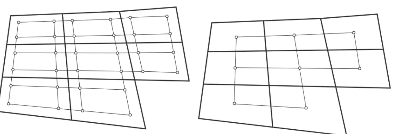
Figure 2: Auxiliary meshes for the SUPG update.

3 THE SUPG TECHNIQUE

We compare the latter method with another one based on the Streamline Upwind Petrov Galerkin technique [3], which was introduced in order to avoid the cross-wind diffusion appearing in the solution of the convection problem. The main idea of the method is the definition of a second mesh defined on the Gauss points. The Lagrangian step is solved on the classical finite element mesh and the convection step is performed on the second mesh by the finite element method and the SUPG technique.

The equation 1 can be written in matrix form (see [1] for more details) :

C ˙u+ K u = 0, (3) with Cij = Z V NiNjdV + Z V k kwk2 wk ∂ Ni ∂ xk NjdV (4) Kij = Z V wkNi ∂ Nj ∂ xk dV + Z V k kwk2 wkwl ∂ Nj ∂ xk ∂ Nj ∂ xl dV (5)

where Ni are the shape functions and k is a diffusion coefficient computed locally by

k = α (| ~w. ~h1| + | ~w. ~h2|), (6)

where α is an upwind parameter and ~h1 and ~h2 are the median vectors of the element

concerned. As in the previous algorithm, an explicit Euler scheme is used for the time integration and the matrix C is diagonalized. It can be shown that it improves the

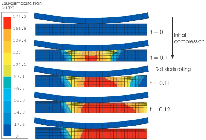
0 17.4 34.8 52.3 69.7 87.1 104.5 122 139.4 156.8 174.2

Equivalent plastic strain [x 10 ]

t = 0

t = 0.1

t = 0.11

t = 0.12

Roll starts rolling Initial

compression

-3

Figure 3: Evolution of the equivalent stress for the Godunov-like update.

4 APPLICATION TO THE ROLLING PROCESS

Both presented algorithms have been tested on a simulation of a cold rolling process. In this case, the ALE formulation is very well suited because we can only study the interesting zone of the process, that is the part of the sheet between the rolls. The problem is symmetric and only one half of the process is studied. The table 1 shows the material properties used for this simulation.

The optimal value for the upwind factor is rather difficult to find. If a low value is chosen, oscillations may appear in the solution. However, a high value introduces too much artificial diffusion.

The roll is a flexible body with the same Young s modulus as the sheet. Only one quarter of the roll is meshed. As far as the mesh of the sheet is concerned, we use an

Young modulus E = 6.895 104 MPa Poisson ratio ν = 0.33 Yield stress σ0 Y = 50.3(1 + εp/0.55)0.26 MPa Rolls radius R = 158.75 mm

Half initial thickness Hi = 6.274 mm

Half final thickness H0 = 5.385 mm

Friction coefficient µ = 0.1 Upwind factor α = 1.0

Table 1: Material properties, geometry and parameters of the rolling process.

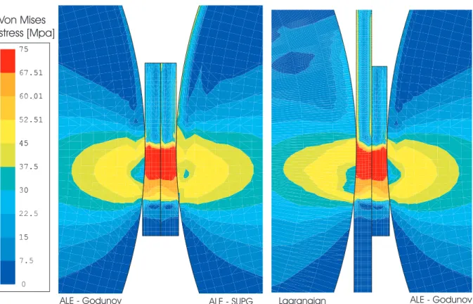
0 7.5 0 7.5 15 22.5 30 37.5 45 52.51 60.01 67.51 75 15 30 37.5 45 52.51 60.01 67.51 75 0 7.5 Von Mises stress [Mpa]

ALE - Godunov ALE - SUPG Lagrangian ALE - Godunov

Eulerian mesh in the rolling direction and a Lagrangian-Eulerian mesh in the perpendic-ular direction. Thus, the free surface of the sheet is automatically computed. The ALE method is used for the sheet and the roll.

The Eulerian domain for the sheet is 60 mm long and discretised with 40 x 6 elements and the roll with 120 x 15 elements. The meshes are refined near the contact area in order to get more accurate results.

The calculation is divided into two steps (see figure 3). The first one consists of the clamping of the sheet by the rolls. Once the desired reduction is obtained, the rolls start to rotate with a constant velocity. The computation is stopped after a rotation of 180 degrees in order to check the stability of both algorithms.

Actually, the steady state is reached rather quickly after a 15 degrees rotation. Its obtained after about 440 time steps. The Godunov-like algorithm is approximately 30% faster than the SUPG method (4 min 40 s instead of 6 min 02 s). The equivalent stress is shown on figure 4. On the left, the Godunov and SUPG updates are compared. We see that the results are very similar. However, the SUPG solution shows more numerical oscillations. On the right, the Godunov update is compared to the equivalent Lagrangian simulation and both solutions are very similar.

5 APPLICATION TO A DRAWBEAD SIMULATION

Another interesting simulation has been considered to compare our update algorithms. In this case, we try to simulate a drawbead test presented by Nine [6], which consist in clamping a thin sheet of metal between three cylindrical rolls and pulling the sheet to make it bend and unbend through the system. This kind of experiment is very important in the deep drawing industry because the forces of such a system are rather difficult to predict.

The geometry and material properties used for the simulation are presented in the table 2.

Young modulus E = 200 GPa

Poisson ratio ν = 0.3 Yield stress σ0

Y = 516(8.2139 10−3+ εp)0.23 MPa

Roll bead radius R1 = 5.5 mm

Roll shoulder radius R2 = 5.5 mm

Friction coefficient µ = 0.0 Upwind factor α = 1.0

Table 2: Material properties, geometry and parameters of the drawbead simulation.

The frictionless case is chosen here for the comparison. This means that the rolls are not fixed and can roll to follow the sheet motion.

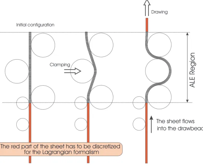
The figure 5 explains the two successive steps during the test. At the beginning, the sheet lies undeformed between the rolls. Then, the clamping phase begins. Once the desired clamping distance is obtained, the drawing phase begins until a stationary solution is computed.

In the case of a Lagrangian simulation, a long part of the sheet must be discretised because the steady state is not obtained immediately. With the ALE formalism, only a small part of the sheet, that is the interesting part, is considered and discretised (this part is called ‘ALE region’ in figure 5). The sheet flows into the ALE mesh.

A

LE

R

e

g

io

n

The sheet flows into the drawbead

The red part of the sheet has to be discretized for the Lagrangian formalism

Figure 5: ALE Region for the drawbead simulation.

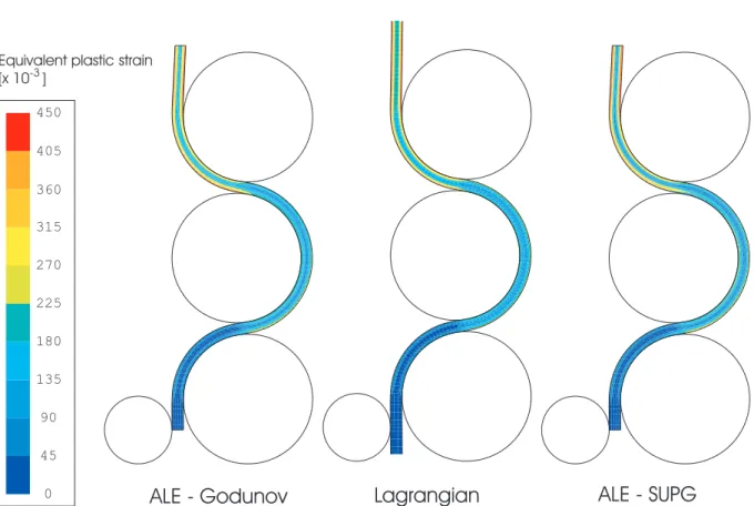
The figure 6 compares the results obtained by both update methods and the Lagrangian case. Once again, we see that the equivalent plastic strain is very similar in the three

0 45 90 135 180 225 270 315 360 405 450

ALE - Godunov Lagrangian ALE - SUPG

Equivalent plastic strain [x 10 ]-3

Figure 6: Comparison of the equivalent plastic strain for the Lagrangian and ALE simulations.

6 CONCLUSIONS

In this paper, two efficient convection algorithms have been introduced in the frame of Arbitrary Lagrangian- Eulerian methods in solid mechanics. They can be very useful when dealing with stationary processes like rolling. However, these results cannot be extended easily to unstructured meshes.

REFERENCES

[1] R. Boman. Formalisme Eul´erien Lagrangien pour le contact lubrifi´e entre solides (Rapport d’activit´e FRIA — in French). Technical Report TF-55, Universit´e de Li`ege, Belgium, 1998.

[2] R. Boman and J.-P. Ponthot. ALE methods for stationary solutions of metal forming processes. In J.A. Cavas, editor, Second ESAFORM conference on Material Forming, pages 585–589, Guimaraes, Portugal, 1998.

[3] A. N. Brooks and T. J. R. Hughes. Streamline upwind/petrov-galerkin formulations for convection dominated flows with particular emphasis on the incompressible navier-stokes equations. Computer Methods in Applied Mechanics and Engineering, 32:199– 259, 1982.

[4] F. Casadei, J. Donea, and A. Huerta. Arbitrary lagrangian eulerian finite elements in non-linear fast transient continuum mechanics. Technical Report EUR 16327 EN, University of Catalunya, Barcelona, Spain, 1995.

[5] A. Huerta. ALE stress update in transient plasticity problems. In E. Hinton D.R.J. Owen, E. Onate, editor, Computational Plasticity, pages 1865–1871. 1995. [6] H.D. Nine. The applicability of Coulomb’s friction law to drawbeads in sheet metal

forming. Jounal of Applied metal Working, 2:200–210, 1982.

[7] J-P. Ponthot. Traitement unifi´e de la M´ecanique des Milieux Continus solides en grandes transformations par la m´ethode des ´el´ements finis (in French). PhD thesis, Universit´e de Li`ege, Li`ege, Belgium, 1995.

[8] J.-P. Ponthot and M. Hogge. The use of the Eulerian-Lagrangian FEM in metal forming applications including contact and adaptive mesh. Winter Annual Meeting, Atlanta, USA, 125:44–64, 1991.