HAL Id: hal-01182410
https://hal.inria.fr/hal-01182410
Submitted on 3 Aug 2015HAL is a multi-disciplinary open access archive for the deposit and dissemination of sci-entific research documents, whether they are pub-lished or not. The documents may come from teaching and research institutions in France or abroad, or from public or private research centers.
L’archive ouverte pluridisciplinaire HAL, est destinée au dépôt et à la diffusion de documents scientifiques de niveau recherche, publiés ou non, émanant des établissements d’enseignement et de recherche français ou étrangers, des laboratoires publics ou privés.
systems
Marc Bouissou, Hilding Elmqvist, Martin Otter, Albert Benveniste
To cite this version:
Marc Bouissou, Hilding Elmqvist, Martin Otter, Albert Benveniste. Efficient Monte Carlo simu-lation of stochastic hybrid systems. The 10th International Modelica Conference 2014, Hubertus Tummescheit; Karl-Erik Årzén, Mar 2014, Lund, Sweden. �10.3384/ECP14096715�. �hal-01182410�
Efficient Monte Carlo simulation of stochastic hybrid systems
Marc Bouissou
1,5, Hilding Elmqvist
2, Martin Otter
3, Albert Benveniste
41
EDF R&D, 1 av. du Général de Gaulle, 92141 Clamart, France
2
Dassault Systèmes AB, Ideon Science Park, SE-223 70 Lund, Sweden
3
DLR, Institute of System Dynamics and Control, D-82234 Wessling, Germany,
4
IRISA/INRIA, Campus de Beaulieu, 35042 Rennes Cédex, France
5
Ecole Centrale Paris, Grande Voie des Vignes, 92295 Châtenay Malabry, France
[email protected], [email protected], [email protected], [email protected]
Abstract
This paper proposes an efficient approach to model stochastic hybrid systems and to implement Monte Carlo simulation for such models, thus allowing the calculation of various probabilistic indicators: relia-bility, availarelia-bility, average production, life cycle cost etc. Stochastic hybrid systems can be considered, most of the time, as Piecewise Deterministic Markov Processes (PDMP). Although PDMP have been long ago formalized and studied from a theoretical point of view by Davis (Davis 1993), they are still difficult to use in real applications. The solution proposed here relies on a novel method to handle the case when the hazard rate of a transition λ depends on continuous variables of the system model, the use of an extension of Modelica 3.3 and on Monte Carlo simulation. We illustrate the approach with a simple example: a heating system subject to failures, for which we give the details of the modeling and some calculation results. We compare our ideas to other approaches reported in the literature.
Keywords: Stochastic hybrid system; PDMP; dynamic reliability; state-dependent hazard rate; continuous time state-machine; Monte Carlo Simula-tion.
1 Introduction
Usually, Modelica models are deterministic; they are built to simulate the nominal behavior of the systems they represent. In order to challenge the functioning of these systems in diverse situations, or in the pres-ence of a varying environment, a degree of random-ness is sometimes added to the system inputs.
But the kind of models this paper is dedicated to is quite different: here, the random behavior can be due to the system itself, mainly because of failures and repairs of components. The purpose of reliabil-ity, and more generally, of dependability studies is to
calculate probabilities of undesirable events such as the failure of the mission of a system, or to estimate the probability distribution of some performances of the system: total production on a given time interval, maintenance cost, number of repairs etc. Usually, dependability studies are performed with dedicated methods and tools, based on discrete (and often even Boolean) models of systems: fault trees, Markov chains, Petri nets, etc.
However, in some situations, a purely discrete representation of a system cannot be a good enough approximation: this is the case of hybrid systems, having both discrete and continuous parts, with strong interactions between the two. Reliability ana-lysts call the study of such systems "dynamic relia-bility".
Below are two examples showing the need for powerful tools for dynamic reliability studies:
In the probabilistic safety analysis of nuclear power plants, so-called "level 1" studies, that are those aiming at assessing the probability of a core melt, rely on discrete (mainly Boolean) models. But after a core melt, components are subject to physical stresses (temperature, humidity and radioactivity) that may modify their behavior and increase very much their failure rates, and this should be taken into account in "level 2" studies that try to assess the risks of radioactivity release in the environment. Even for level 1 studies, there is a competition in time be-tween the decay of the thermal power that must be evacuated and the failures of components, and the coarse decomposition of scenarios according to large time intervals in which failures can happen can be excessively pessimistic.
Another example of system associated to very high stakes and whose behavior cannot be captured correctly without a stochastic hybrid model is the electrical grid. In this system, transients with ex-tremely different time scales can happen and evolve to blackout situations. For example, after the failure of a line, the intensity increases in the remaining
lines; it can augment their temperature which, be-cause of dilatation, makes them come closer to the ground. This increases the probability of a new fault due to a contact between a line and a tree.
Recent results have shown that numerical schemes can solve PDMP with a small size, however Monte Carlo Simulation remains the only possible method for quantification in larger cases.
The purpose of this paper is twofold: it shows how to model a hybrid stochastic system and it gives an efficient Monte Carlo scheme that works even in the case of failure rates varying with the continuous variables of the system.
2 A review of formalisms used for
hybrid system modeling
In this section, we will first give the theoretical mod-el called PDMP (Piecewise Deterministic Markov Processes). Then we will explain the limits of PDMP and why these limits are not a real problem as long as we intend to model physical systems (and not, for example, financial systems). Finally we will see how some existing formalisms (including Modelica) can be used to represent PDMP.
2.1 The theoretical model PDMP
The state at time t (x(t), m(t))t≥0 of a hybrid system is
composed of two parts: a continuous one,
x t
( )
∈
nand a discrete one,
m t
( )
∈
.x(t) usually models physical variables such as tem-perature, pressure, volume, flow rate, etc., whereas m(t) is the index of the state of the discrete "part" of the system: to each value of m(t), one can associate discrete states (such as working or failed, open or closed etc.) to each component of the system.
What makes the resolution of dynamic reliability problems difficult is the existence of bi-directional interactions between x(t) and m(t). Here are some examples of such interactions:
• x(t) acts on m(t). When a physical variable reaches a threshold, it can provoke a discrete change: explosion of a tank because of high pressure, evaporation of steam because of high temperature, reaction of the instrumentation and control system. A physical variable can also make a discrete event happen earlier or later: for example, a failure rate may increase with the temperature.
• m(t) acts on x(t). The opening or closure of a valve, the failure of a pump changes the differen-tial equations governing physical variables.
From a mathematical point of view, PDMP contain all the ingredients needed to model stochastic hybrid systems such as those exemplified above (Davis 1993).
The general equations governing the evolution of the PDMP whose state is described by (x(t), m(t))t≥0
( ) ( ( ), ( )) Pr( ( ) / ( ) , ( )) ( , , ( )) ( ) = + ∆ = = = + ∆ dx t g x t m t dt m t t j m t i x t λ i j x t o t
Here, λ(i,j,x(t)) denotes a function that defines the hazard1 rate from state i to state j for the discrete part of the system:
× ×
n
λ→
. In other words, it defines the probability that a transition occurs from discrete state i to state j.2.2 Scope and limits of PDMP
The scope of PDMP is quite large: it generalizes all discrete models used in dependability analysis, even those considered as non markovian, (like for exam-ple Petri nets with arbitrary probability distributions for delayed transitions) due to the modeling "trick" explained below.
Thanks to the insertion into x(t) of the time elapsed since the beginning of the life of an aging compo-nent, it is possible to model the probability distribu-tion of the time to failure of this component, whatev-er this distribution may be.
For example, here is how we can transform a non markovian process with two states modeling a com-ponent with a Weibull distributed lifetime into a markovian process, thanks to the addition of time in the definition of the state:
• the "usual" definition (m = 1 corresponds to a working state, and m = 0 corresponds to a failed state):
Pr( ( )
m t
0) 1 exp
( )
t
βα
=
= −
−
(1)In this expression,
α
∈
+* α is the scale factor andβ
∈
+* is the shape parameter of the Weibull distribution.• definition with a PDMP whose continuous vari-able represents the time:
( ) 1 dx t because x t dt = = (2)
1 Here, reliability analysts would rather use the term
"tran-sition rate" instead of "hazard rate". These two expres-sions are synonyms, but we use the second one because it is the most neutral. It is the quantity defined in eq. (6).
1 Pr( ( ) 0 / ( ) 1), t) exp ( ) ( ) m t t m t t t o t β β β α α α − + ∆ = = = − + ∆ (3) Pr( (m t+ ∆ =t) 0 /m t( )=0), t)=1 (4) In equation (3), we use the hazard rate of the Weibull distribution.
This kind of representation by a PDMP can be gen-eralized to any lifetime distribution; the remarkable case when the hazard rate is in fact constant corre-sponds to the exponential distribution (see section 3.1).
The large expressive power of PDMP unfortu-nately comes with a heavy additional burden for ana-lysts: as one can see from the very elementary exam-ple given above, PDMP are not at all easy to ma-nipulate. In fact, they are both difficult to specify, and to solve by methods other than Monte Carlo simulation.
How about their limits? Of course, PDMP do not address all the needs for reliability studies of systems involving uncertain dynamics. Neither random con-tinuous inputs nor measurement noise can be cap-tured. Still, PDMP offer a first interesting step be-yond classical dynamic dependability models with discrete space. PDMP are interesting in that they do not require the modeling and simulation of full fledge stochastic differential equations. Their Monte-Carlo simulation can be performed at reduced cost, as we shall see.
2.3 Modeling in practice
Modeling hybrid systems has long been a concern for the study of purely deterministic systems.
For relatively simple models, the graphical repre-sentations used in control and signal processing can suffice. They allow the graphical construction of transfer functions, using assemblies of elementary blocks representing integrators, differentiators, mul-tipliers, adders, thresholds etc.
For more complex models, a higher level of ab-straction is needed. This can be achieved by the en-capsulation of algebraic, differential and discrete equations in objects corresponding to physical com-ponents. This is the solution made possible by Mod-elica. Thanks to Modelica libraries, it is possible to quickly build models of mechanical, electrical, fluid etc. systems, encompassing thousands of equations. However, so far this kind of representation has not been extended to allow a convenient modeling of stochastic hybrid systems.
Thanks to a comparison between various existing modeling languages for PDMP done in (Bouissou
and Jankovic 2012) and (Bouissou et. al. 2013), the missing features in Modelica 3.3 can be identified: • Asynchronous state machines in which
transi-tions are triggered by events (instead of synchro-nous state machines triggered by a clock) • Transitions that can be associated to random
de-lays (this is the most important and delicate point)
• Allowing several instantaneous transitions from one state having specified probabilities of firing. Section 4 will describe the two first points in detail2, but before that, we will give what is in fact the main point of this paper: a smart algorithm allowing to perform Monte Carlo simulation on PDMP. This algorithm is usable whatever the interactions be-tween the discrete and continuous parts of the pro-cess and is very economical in terms of CPU usage.
3 Making the Monte Carlo
simulation of a PDMP efficient
3.1 State of the art
The state of the art Monte Carlo simulation method for PDMP is described in (Zhang et al. 2008). This paper recalls the mathematical definition of PDMP as it was set up by Davis and gives an iterative simu-lation algorithm that determines the successive times of process jumps due either to a random event or to the fact that the continuous part of the system reach-es the boundary of the currently valid domain for the differential equations.
Starting from the initial state of the system, the first jump date is the minimum of the dates of the set of events corresponding to:
- Boundaries crossings: the corresponding dates are obtained by solving the current set of differ-ential equations until one of the continuous vari-ables crosses a threshold;
- Random events. In most cases, there is a compe-tition between several transitions associated to individual probability distributions of the times to firing of these transitions (like in a stochastic Petri net). For example, several components can fail at any moment, but if their failures are inde-pendent, one will fail first, and this will deter-mine the instant of the first jump date.
When the random processes are independent from continuous variables, it is easy to determine, at t=0,
2
The third point will not be developed in this article, both because of a lack of space and because it is not related to the two other points.
the dates of all random events (details given hereaf-ter). But if they are not, their determination is more difficult. We will first recall the definition of the hazard rate, associated to the distribution of any ran-dom variable such as the time to a failure or a repair then explain a method able to find in one run, with-out any backtrack, the date of the first event in the system, whatever its nature (random of boundary crossing).
Given a random time T whose cumulative distribu-tion funcdistribu-tion (cdf) F is defined as
𝐹(𝑡) = Pr (𝑇 < 𝑡) (5)
the corresponding hazard rate, λ(t), is defined as:
0 Pr( | ) ( )
lim
t T t t T t t t λ ∆ → < + ∆ > = ∆ (6)The hazard rate can then be expressed as
𝜆(𝑡) =1 − 𝐹(𝑡)𝐹′(𝑡) (7)
that is 𝑑𝐹(𝑡)
𝑑𝑡 = (1 − 𝐹(𝑡))𝜆(𝑡) (8)
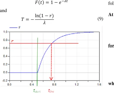
For Monte Carlo simulation, the time to the next event, T, is determined by drawing a uniform random number, r in [0,1], and solving:
𝐹(𝑇) = 𝑟
When λ is constant, the solution to the differential equation (7) is:
𝐹(𝑡) = 1 − 𝑒−𝜆𝑡
and
𝑇 = −ln (1 − 𝑟)𝜆 (9)
Figure 1: The "inverse cdf" technique for drawing a ran-dom number according to a given distribution
In figure 1, this approach is visualized (here: tstart is
the time instant when the random number r is drawn,
and tfire is the time instant of the stochastic event, so
T = tfire - tstart, the blue curve is the cumulative
distribution function F).
When the hazard rate of a transition depends on con-tinuous variables x, so, 𝜆(𝑡, 𝑥(𝑡)), the cumulative distribution function F can be obtained by integra-tion of eq. (7) and is equal to
𝐹(𝑡) = 1 − 𝑒− ∫ 𝜆(𝑢)𝑑𝑢0𝑡 (9)
Then, the usual and "naïve" way to proceed is to in-tegrate the differential equations up to a "large enough" time, draw a uniform random number r and calculate T as
F
−1( )
r
.This process involves solving the differential equa-tions of the model during a sufficiently large time interval and calculation of λ(t) which is dependent on variables of the model. A numerical method is then used for integration of λ(t) followed by calculation of F(t). After this, the integrator of the differential equations needs to be rewound to tfire, an operation
normally not present in numerical integration meth-ods.
3.2 New method for state dependent hazard rates
Instead of this complex and slow procedure, a new method has been developed that utilizes the fact that F is monotonically increasing and the zero crossing solver for events available in modern integration rou-tines can be used to find the next event time 𝑡𝑒,𝑖+1. The complete set of equations can be defined in the following way: At event 𝑡 = 𝑡𝑒,𝑖: 𝑚�𝑡𝑒,𝑖� = 𝑔�𝑚�𝑡𝑒,𝑖−1�, 𝑡𝑒,𝑖� 𝐹�𝑡𝑒,𝑖� = 0 𝑟�𝑡𝑒,𝑖� = 𝑟𝑎𝑛𝑑𝑜𝑚() for 𝑡𝑒,𝑖 < 𝑡 < 𝑡𝑒,𝑖+1: 0 = 𝑓 �𝑥̇, 𝑥, 𝑦, 𝑡, 𝑚�𝑡𝑒,𝑖�� 𝐹̇ = (1 − 𝐹) ∙ 𝜆 �𝑥̇, 𝑥, 𝑦, 𝑡, 𝑚�𝑡𝑒,𝑖�� 𝑡𝑒,𝑖+1= min𝑡>𝑡 𝑒,𝑖𝑡, such that 𝐹 ≥ 𝑟�𝑡𝑒,𝑖� where 𝑡 ∈ ℝ, 𝑥(𝑡) ∈ ℝ𝑛𝑥, 𝑦(𝑡) ∈ ℝ𝑛𝑦, 𝐹(𝑡) ∈ ℝ 𝑚�𝑡𝑒,𝑖� ∈ ℕ, 𝑓(. . )∈ ℝ𝑛𝑥+𝑛𝑦,𝜆(. . ) ∈ ℝ
This system consists of a continuous-time DAE (Dif-ferential Algebraic Equation system) defining the physical model, together with a state machine. The active state of the state machine is characterized by
the integer variable m. The DAE is a function of this active state m, and of continuous-time states x and algebraic variables y.
At an event instant 𝑡 = 𝑡𝑒,𝑖 a transition to the next state of the state machine occurs, the cumulative distribution function F is re-initialized to zero, and a random number r is drawn.
Afterwards the DAE together with the differential equation for F is integrated until
𝐹(𝑡) − 𝑟�𝑡𝑒,𝑖� = 0
This means that the zero crossing of 𝐹(𝑡) − 𝑟�𝑡𝑒,𝑖� triggers a state event3 and the corresponding (sto-chastically determined) time instant is the next event instant 𝑡𝑒,𝑖+1.
For notational convenience this description was given for a special case. It is easy to generalize for several state machines where one or more stochastic and/or deterministic transitions are defined at the active states.
Remark: the above approach can be seen as a generalization of the simulation of nonhomogeneous Poisson processes (Sheldon 1990). Indeed, two methods of generating a Poisson process with known time-varying hazard rate function 𝜆(𝑡) are proposed in Section 5.5 of this reference, of which the second one can be seen as a basis of our method: it is pro-posed in Section 5.5 to compute
𝐹(𝑡 − 𝑡𝑒) = 1 − 𝑒− ∫ 𝜆(𝑢)𝑑𝑢
𝑡−𝑡𝑒 0
and then to invert the equation 𝐹(𝑡 − 𝑡𝑒) = 𝑟(𝑡𝑒) for t, where r is a random number drawn at the last event time 𝑡𝑒. We propose to differentiate the above equa-tion, thus making clear that the time-varying intensi-ty 𝜆(𝑡) can be given on-line. With this observation, we can now allow that 𝜆(𝑥̇, 𝑥, 𝑦, 𝑡, 𝑚) is a function of the variables of a DAE describing the physical sys-tem, F is computed by integrating the differential equation for F together with the system DAE, and the stochastic event time is computed as the state event where F ≥ r becomes true. We discovered our method independently, however, and this reference was subsequently pointed to us by Pierre Brémaud.
4 Modeling PDMP in Modelica
In this section it is shown how PDMP can be mod-eled in Modelica and how Monte Carlo simulations can be carried out over such models. Furthermore,3 State events are supported by modern ODE and DAE
solvers; the solver will automatically iterate around the time instant where this function crosses zero, will back-track, and will find the event time up to a certain preci-sion.
with the novel technique from section 3.2 it is possi-ble to model hazard rates that depend on the states of continuous variables in an efficient way.
4.1 Overview
In Modelica 3.3 support for hierarchical, synchro-nous, clocked, state machines (Elmqvist et.al. 2012) was added. Such state machines are evaluated at clock ticks of sampled data systems, and are now the preferred way to model state machines in Modelica. In a prototype of Dymola, this state machine type was extended to model also continuous-time state machines (Elmqvist et.al. 2014) and is the basis for the PDMP implementation in Modelica.
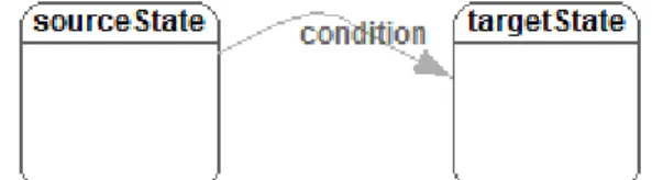
The basic mechanism is a generalization of transi-tions in the Modelica synchronous state machines, as sketched in the following figure:
Figure 2: Transition between two states in a state machine A transition in a Modelica 3.3 synchronous state ma-chine fires, if its source state is “active” and the tran-sition “condition” becomes true. If trantran-sition flag “immediate=true”, the transition fires immediately (so at the same clock tick). If “immediate=false”, the actual firing occurs at the next clock tick, so it is de-layed. This approach is generalized in the following way for continuous-time asynchronous state ma-chines:
- If “immediate=true”, the behavior is as before, so the transition fires immediately (at the current model evaluation).
- If “immediate=false”, by default a new event iteration is triggered and the transition fires at the next event iteration (so with an infinitesimal small delay that breaks algebraic loops).
There are several useful ways to delay a transition, such as by a fixed time period (e.g. firing after 2ms), or by a time period that is defined stochastically in different ways (as needed for a PDMP). Since there are many possibilities, it seems not possible to pre-define this behavior in a language element, but it needs to be configurable by a user.
In the following sub-sections, the different ingre-dients needed for such a Modelica extension are dis-cussed.
4.2 Random number generation
In order to draw random numbers for the triggering of stochastic transitions, a random number generator is needed. A standard random number generator in a programming language is an impure function and is typically called as “r = random()”, so the function has no arguments and returns for every call a differ-ent random number, typically in the range 0 ≤ r ≤ 1. It is clear that such a function cannot be implement-ed as a Modelica function, because Modelica func-tions are “pure”, and return always the same value, when called with the same input arguments. There are the following remedies:
(1) Explicitly pass the internal memory (usually called “seed”) of the random number function as input and output arguments:
(r, seed) = random(pre(seed))
As a result, the random function can return a dif-ferent (r, seed) value only at an event instant, as it should be, because the operator pre(..) can only be used in a discrete equation. It is therefore guaranteed that the random number function cannot be called during continuous in-tegration which would give severe problems with the integration method.
(2) Use an external Modelica function as interface to a C-function, r = random(), and mark this func-tion as impure:
impure function random output Real r;
external "C" r = random(); end random;
The “impure” keyword introduced in Modelica
3.3 guarantees that the random function can be basically only called in a when-clause, so at event instants.
Calling a random number generator in any simula-tion environment is tricky, because there are differ-ent requiremdiffer-ents and depending on the analysis, simulation runs should (a) use different random number sequences in every simulation run, as for Monte Carlo simulations, or (b) should use the same random number sequences in specific simulations, as for Optimization over Monte Carlo simulations (Looye, Joos 2006) or when developing a model.
option 1 option 2
Figure 3: Two options for the pseudo random generator
Taking into account the above observations, a Mod-elica model was designed to define the random prop-erties globally: The user has to drag model “Glob-alSeed” in the model and can then select from two options: in the first case (by default), for every simu-lation run a different initial seed is selected. In the second case, defined by a flag, initial seeds can be explicitly defined and every simulation run will use the same random number sequence. The selected seeds are displayed in the icon.
In a model, the random number generation func-tion is called in the following way:
protected
outer GlobalSeed globalSeed; Real r "random number"; equation
when condition then
r = globalSeed.random(); end when;
Since globalSeed.random is defined as an impure function, it can only be called in a when clause, so only at an event instant. Every call returns a different number in the range 0 ≤ r ≤ 1.
4.3 Delayed transition blocks
As already mentioned, there are many ways to define the delay of a transition. In order to keep this user configurable, it is proposed to define the delay by a Modelica block, with one Boolean input and one Boolean output signal, which has the following properties:
The input signal of such a block, called enable-Fire, signals when the source state is active and the transition condition becomes true. The signal is then set to true, until it is explicitly reset (either because the transition fired, or the source state became inac-tive, e.g., due to the earlier firing of another transi-tion).
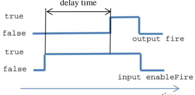
Figure 4: Behavior of a delay block
The delay block triggers an event after a defined “de-lay time” and at this time instant the output signal fire is set to true. This raising signal triggers the firing of the transition. Immediately, when the source
time delay time output fire input enableFire false true false true
state becomes inactive, enableFire and fire are both reset to false.
Based on this principle, a small library of delay blocks has been implemented. The two deterministic delay blocks FixedTimeDelay and Variable-TimeDelay define the delay by a fixed or variable deterministic time delay, respectively. The core part of the FixedTimeDelay block implementation is (t_start is the time instant when the input enable-Fire is rising4):
if enableFire then
fire = time >= t_start + delayTime;
else
fire = false;
end if;
Therefore, a time event is triggered after the defined delayTime and the output fire changes to true at
this time instant. Conceptually, the equations in a transition are defined as:
algorithm
when initial() then
enableFire := stateActive and condition;
elsewhen stateActive and condition then enableFire := true;
elsewhen not stateActive then enableFire := false; end when; equation if immediate then fire = enableFire; else delayBlock.enableFire = enableFire; fire = pre(delayBlock.fire);
end if;
Note, the output fire of the delay block needs to have an infinitesimal small delay via the pre(..) operator in order to break algebraic loops.
4.4 Randomly delayed transitions
The approach sketched in section 3 for fixed (not state-dependent) hazard rates leads the following implementation in Modelica, where the implementa-tion of eq. (9) can be easily identified:
outer GlobalSeed globalSeed; Real r, t_next;
parameter Real hazardRate; equation
when enableFire then
r = globalSeed.random();
t_next = time – log(1-r)/hazardRate; end when;
4
At the time instant where enableFire becomes true, the actual value of the variable delay time is inquired and this value is used as delay time.
if enableFire then
fire = time >= t_next; else
fire = false; end if;
Since the condition time >= t_next is a purely time dependent condition, a Modelica tool will determine the time instant of the fire time in advance and will directly (and therefore efficiently) integrate to this time instant.
Other stochastic distributions can be implemented in a similar way, provided that the distribution of the time to the firing is invariant once the enableFire Boolean has become true.
4.5 State dependent
randomly delayed transitions
In this section the implementation of the innovative approach from section 3.2 is sketched: the corre-sponding delay block can be defined in Modelica as:
outer GlobalSeed globalSeed; Real r;
input Real hazardRate(min=0); equation
when enableFire then
r = globalSeed.random(); reinit(F,0); // start at F=0 end when; der(F) = (1-F)*hazardRate; if enableFire then fire = F >= r; else fire = false; end if
The expression F >= r defines a state event and will therefore trigger a search process to determine the time instant when this condition becomes true up to a certain numerical precision. At this time instant an event is triggered.
4.6 Asynchronous state machines
As already mentioned, in a prototype of Dymola the Modelica 3.3 synchronous state machines have been extended to continuous-time (= asynchronous) state machines. For all details see (Elmqvist et.al. 2014). As a very short summary: the states of a state ma-chine might be non-clocked Modelica models or blocks. The “active” state is always simulated to-gether with the rest of the DAE system and all out-going transitions from this state are monitored. If one of these transitions fires, an event is triggered, the active state is changed and simulation continues with the new active state. All de-activated state models or blocks are “frozen”, so all variables in these objects
keep their values until these states become again “ac-tive”.
In Modelica 3.3 a transition is defined with the following built-in operator (see Modelica 3.3 speci-fication, section 17.1):
transition(from, to, condition, immediate, reset, synchronize, priority)
Here “from” and “to” are the instance names of the blocks used as source and target state of the transi-tion, “condition” is the firing condition and “imme-diate” is the flag that defines whether the transition is immediately firing or is firing at the next clock tick (the remaining arguments are not important for the following discussion).
This “transition” operator holds in principal also for continuous-time state machines. However, the case for “immediate=false” needs to be differently defined: As sketched in the previous sections, a wide variety of useful delay definitions can be provided by different blocks. Therefore, one approach would be to use a replaceable block as additional argument in the transition operator. Example:
transition(“state1”,“state2”,true,false,true,true,1, redeclare FixedHazardRateDelay delay(hazardRate=0.03)); This call would use block “FixedHazardRateDelay” for the block instance “delay” with the given modifi-er. Built-in operators in Modelica have the syntax of a function call. However, a block, being replaceable or not, cannot be passed to a function, and therefore, this construct seems to be unnatural to a built-in op-erator. It would be possible to pass a function object, such as:
transition(“state1”,“state2”,true,false,true,true,1, delay = function FixedHazardRateDelay (hazardRate=0.03)); However, with a function object, it would not be possible to define stochastic transitions that depend on continuous-time states (see section 4.5) because a differential equation needs to be solved in the object and state events need to be triggered.
It is therefore proposed to define the transition built-in operator with a syntax that is close to the function object:
transition(“state1”,“state2”,true,false,true,true,1, delay = block FixedHazardRateDelay (hazardRate=0.03)); Informally, the semantics is that the provided block (here: FixedHazardRateDelay) with its modifier is instantiated in the scope of the source state, so this block is only active and running, when its source
state is active and otherwise is “frozen”. If a delay block is not explicitly given, the default block will just implement the equation
fire = pre(enableFire);
so an infinitesimal small delay will be introduced. Unfortunately, such a built-in operator is uncom-mon in Modelica (having a replaceable block as an argument to a built-in operator) and it is unclear whether this complicated definition should be intro-duced into the Modelica language specification.
For this reason, another approach is used in the prototype: The desired delay block is instantiated inside the source state. In the transition, the output of the delay block is utilized. The implementation in the source state is basically straightforward by instantiat-ing from the desired delay block:
FixedHazardRateDelay delay(
enableFire=enteringState(), hazardRate=0.3);
An issue is to define, when the random number shall be drawn (that is, when the input enableFire has a rising edge). In the prototype, enableFire is defined to have a rising edge, when the source state is en-tered. This is inquired, with the (not yet standard-ized) built-in operator “enteringState()”, that is available as a prototype in Dymola. As transition condition simply “<source-state>.delay.y” is used.
5 Case study
5.1 Preamble
The test case we are going to use to illustrate our ideas was first used to screen a number of potential tools and approaches adapted to dynamic reliability (Bouissou and Jankovic 2012), (Bouissou et al 2013) It has the advantage that it is easy to understand.
Although this test-case is very simple it has been quite difficult to solve it with tools that were initially designed only for modeling deterministic systems (and this includes Modelica tools). We intend to solve a more complex test-case in the future, such as the well-known "heated tank" problem used by T. Aldemir in (Aldemir 1991), that has been solved since then with many different approaches e.g. (Lair et. al. 2010), (Zhang et. al. 2008), (Broy et. al. 2011), (Zhang et. al. 2013).
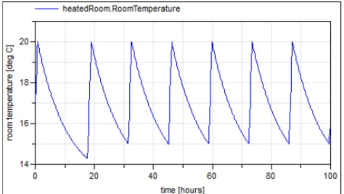
5.2 The "heated room" test case
Consider a room containing a heater. A temperature sensor with a hysteresis switches the heater on when the ambient temperature falls below 15°C and switches it off when the temperature reaches 20°C.
The outside temperature is constant: 13°C. At time t = 0, the temperature of the room is 17°C, and the heater is on.
The flow of energy (power) traversing the walls is proportional to the difference of temperature be-tween the inside and the outside of the room. When the heater is on, it injects a constant power in the
room. Let us suppose that the isolation of the room and the heater power are such that the differential equation giving the evolution of the temperature is as follows (with t in hours, and T in °C):
In this expression, heater_is_on is an indicator func-tion, with the value 1 if the heater delivers power and 0 otherwise.
If the heater was not subject to failures, the trajec-tory of temperature as a function of time would be a deterministic succession of portions of exponential functions, alternatively convex and concave, "oscil-lating" between 15 and 20 °C.
But in fact, the heater has a constant failure rate λ = 0.01/h, and a constant repair rate µ= 0.1/h. How does this random behaviour affect the evolution of the temperature?
6 Modelica models for the case study
The system consists of 5 classes: globalSeed (de-scribed in section 4.2) heaterController, heater, out-sideWeather and heatedRoom. There is only one ob-ject of each class.Figure 5. Structure of the Modelica model
In this case we can have a causal model, where each box has outputs calculated from its inputs. This is why the links are all directed.
The box outsideWeather just contains a constant parameter: the outside temperature, set to 17°C; this value is sent to heatedRoom. In heatedRoom there is the differential equation:
equation
der(T)= 0.1*(Outside_Temperature-T)
+ 5 * Heater_is_on;
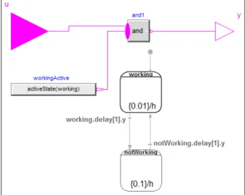
The box heaterController just contains a hysteresis taken from the Modelica standard library. The two bounds (minimal and maximal temperatures respec-tively set to 15 and 20) are defined in this box. The output is a Boolean sent to the box heater; this Bool-ean is true whenever the heater is supposed to heat. 6.1 Heater model with stochastic transitions With the method sketched in section 4, the heater is modelled as a continuous-time state machine where stochastic delay blocks with constant hazard rates are used inside the states (Figure 6).
For example “working” is the state when the heater is working. Inside this state a vector of delay blocks with fixed hazard rates are defined and the hazard rates are displayed in the icon ({0.01}/h), so defining here 0.01 failures per hour. This state is in-stantiated with one delay block, and the transition from “working” to “notWorking” is just referencing the output of this delay block (working.delay[1].y).
Figure 6: The heater model with a continuous-time state machine. In every state an instance of a delay block with constant hazard rate is present. In the transitions, the out-puts of these delay blocks trigger the firing of the transi-tions.
This output becomes true after the stochastic delay defined by the hazard rate (a random number is drawn when state “working” is entered). In this case the state machine switches to “notWorking”. The repair rate is defined as 0.1 failures/h and the state switches back to “working” again, after this stochas-tic delay. The output of the heater model is true, if the state machine is in state “working” and the input of the heater (the signal coming from the controller) is true. The result of one simulation of the overall system is shown in figure 7.
0.1 ( _ ) 5 ( _ _ )
dT
Outside temperature T heater is on
6.2 Monte Carlo Simulation
The above model can directly be used to simulate one realization of the random process corresponding to the life of the system. To perform a Monte Carlo simulation to estimate, for example, the mean tem-perature as a function of time, it is necessary to gen-erate a large number of such trajectories using differ-ent initial seeds for every simulation. This task can be performed in Dymola by using appropriate script functions (that are based on the algorithmic part of the Modelica language). A special Modelica/Dymola script has been implemented for this case to run the simulations and store the desired fractiles5. In figure 8, the mean value of the room temperature is shown, as well as the 1% and 99% fractiles at each time point respectively. 10 000 simulations were per-formed with 500 output points per simulation. On a notebook, these simulations took 25s. Computing the result values for figure 8 took another 45s (the rea-son is that a very simple algorithm was implemented to compute the fractiles and a better implementation will give a considerable speed-up).
Figure 7: A single random trajectory of the temperature (containing one failure and one repair over 100 hours).
Figure 8: Statistics obtained from 10000 trajectories
5 The computation of the 99 % fractile z from 10000
simu-lation runs means that at every grid point of the result 10000 result points are available and that 99 % of these are smaller than z. In other words, 1 % of 10000 values = 100 values are larger than z.
7 Comparison with approaches in the
literature
The same problem (heated room) had been already modelled and solved with three other tools. The de-tails about these experiments can be found in the two ESREL papers already mentioned.
The tool Vensim, which is well known in the do-main of so called "system dynamics" was originally designed for modelling deterministic differential equations. Its graphical input interface is extremely limited, does not allow encapsulation of models, nor reuse by another means than copy-paste. This tool is not usable for real size systems, the building of mod-els being much too error prone.
The tool KB3, based on the Figaro modeling lan-guage, is dedicated to the construction of discrete state stochastic models, for reliability and dependa-bility calculations. With this tool it has been very easy to build a graphical model representing the heated room, using a library for hybrid stochastic Petri nets. The model was solved using the YAMS Monte Carlo simulator, able to process any Figaro model. The main concern with this approach is the impossibility to "separate" in the processing the cal-culations on the discrete and on the continuous part of the model. Thus it would probably be inefficient in terms of CPU consumption on a large model, just like the approach described in (Zhang et al. 2013), commented 15 lines below).
Finally, the tool PyCATSHOO based on Python libraries had also been tested. This tool is new and has no graphical interface. However, it uses an object oriented approach such as Modelica, with two dis-tinct hierarchies, corresponding to the relations "is included in" and "inherits from". The PyCATSHOO models include a native notion of stochastic transi-tion, since this tool was designed specifically for solving dynamic reliability problems. Its scalability is ensured by the use of state of the art libraries for solving differential equations and parallelisation of computations.
It will be interesting to make further comparisons of Modelica and PyCATSHOO models resolutions for larger systems.
In (Aldemir 1991) a more complex benchmark is described. From the solutions to this well-known benchmark (already mentioned in section 5.1), the one from (Zhang et.al. 2013) is interesting, because here a general purpose continuous-time modeling environment (Simulink) is used together with a state machine (Stateflow) to solve a problem with a state dependent hazard rate. However in this reference, a fixed time step integration is utilized for the simula-tion and in every step the approximasimula-tion is used that
the hazard rate is constant. The constant hazard rate is integrated over every time step and at the end of every time step random numbers are drawn to check whether the failures of components are to be trig-gered in the next time step, according to the current values of components failure rates. This technique is less precise and requires a lot more computations compared to the one explained in (Zhang and al. 2008). This seems to be the price to pay in order to be able to use high level models with a small model-ing effort instead of ad hoc programs developed at a high cost in terms of manpower. But in fact, our new approach from section 3.2 is an improvement of the simulation strategy given in (Zhang and al. 2008), without backtracking and able to use error con-trolled, variable step-size integrators for the continu-ous part of the system and yet it allows the use of high level models, as usual in a Modelica environ-ment.
8 Conclusions
In this paper we have pinpointed the need for con-sidering probabilistic safety analyses in which the fault occurrence and propagation behavior can de-pend on the physical and control state of the consid-ered system. Indeed, we advocated that reliability modeling should not be kept separate from modeling of physics and control, as it is today. One specific subtlety of the subject is that the joint consideration of reliability and physics require being able to con-sider state dependent hazard rates for time to failure distributions. As a first contribution, we provided an on-line procedure for Monte-Carlo simulation of such phenomena in the presence of coupling between fault events and system physics. Then, we proposed an extension of the Modelica language to support this kind of modeling. The extension has been meant minimal in that it most possibly relies on existing features. Not all probabilistic phenomena relevant to the joint simulation of reliability and physics are covered by our proposal, but we believe it is a first and significant contribution addressing a large part of the remaining open issues with current approach-es.
9 Acknowledgements
This article is based on work carried out within the ITEA2 project MODRIO. Partial financial support of The German BMBF, the French DGCIS, and the Swedish VINNOVA for this development are highly appreciated.
References
Aldemir T (1991): Utilization of the Cell-to-Cell Mapping
Technique to Construct Markov Failure Models for Process Control Systems, PSAM Proceedings, Elsevier
Publishing Company Co. Inc., NY, pp 1431-1436. Bouissou M., Jankovic M. (2012): Critical comparison of two
user friendly tools to study Piecewise Deterministic Markov Processes (PDMP). ESREL 2012, Helsinki.
Bouissou M., Chraibi H., Chubarova I. (2013): Critical
compar-ison of two user friendly tools to study Piecewise De-terministic Markov Processes (PDMP): season 2.
ESREL 2013, Amsterdam.
Davis M.H.A (1993): Markov Models and Optimization, Chapman& Hall
Elmqvist H., Gaucher F., Mattsson S.E., Dupont F. (2012): State
Machines in Modelica. Modelica'2012 Conference,
Mu-nich, Germany, Sept. 3-5, 2012. Download:
http://www.ep.liu.se/ecp/076/003/ecp12076003.pdf
Elmqvist H., Mattsson S.E., Otter M. (2014): Modelica
exten-sions for multi-mode DAE systems. Modelica'2014
Con-ference, Lund, Sweden, March 10-12.
Looye G., Joos H.D. (2006): Design of Autoland Controller
Functions with Multi-objective Optimization. Journal
of Guidance, Control, and Dynamics, Vol. 29, No. 2, March-April, pp. 475 -484.
Marseguerra M. and E. Zio (1996): Monte Carlo Approach to
PSA for dynamic process system. Reliability
Engineer-ing and System Safety, 52:227-241.
Sheldon M.R. (1990): A course in simulation. Mc Millan, ISBN 0-02-403891-1
Tuffin B., D. S. Chen, and K. Trivedi (2001): Comparison of
hybrid systems and fluid stochastic Petri nets. Discrete
Event Dynamic Systems, 11 (1/2):77-95.
Zhang H., Dufour F., Dutuit Y., and Gonzalez K. (2008):
Piece-wise deterministic Markov processes and dynamic re-liability. Proceedings of the Institution of Mechanical
En-gineers, Part O: Journal of Risk and Reliability 222(4), 545–551.
Zhang H., Saporta B., Dufoura F., and Deleuzed G. (2013):
Dy-namic Reliability by Using Simulink and Stateflow.