HAL Id: hal-01265958
https://hal.inria.fr/hal-01265958
Preprint submitted on 1 Feb 2016HAL is a multi-disciplinary open access
archive for the deposit and dissemination of sci-entific research documents, whether they are pub-lished or not. The documents may come from teaching and research institutions in France or
L’archive ouverte pluridisciplinaire HAL, est destinée au dépôt et à la diffusion de documents scientifiques de niveau recherche, publiés ou non, émanant des établissements d’enseignement et de recherche français ou étrangers, des laboratoires
Wait-freedom and Locality are not Incompatible (with
Distributed Ring Coloring as an Example)
Armando Castañeda, Carole Delporte, Hugues Fauconnier, Sergio Rajsbaum,
Michel Raynal
To cite this version:
Armando Castañeda, Carole Delporte, Hugues Fauconnier, Sergio Rajsbaum, Michel Raynal. Wait-freedom and Locality are not Incompatible (with Distributed Ring Coloring as an Example). 2016. �hal-01265958�
Wait-freedom and Locality are not Incompatible
(with Distributed Ring Coloring as an Example)
Armando Casta˜neda† Carole Delporte‡ Hugues Fauconnier‡
Sergio Rajsbaum† Michel Raynal⋆,◦
†Instituto de Matem´aticas, UNAM, M´exico D.F, 04510, M´exico ‡LIAFA, Universit´e Paris 7 Diderot, 75205 Paris, France
⋆ Institut Universitaire de France
◦ IRISA, Universit´e de Rennes, 35042 Rennes Cedex, France
{cd,hf}@liafa.univ-paris-diderot.fr [email protected] [email protected] [email protected]
Tech Report #2033, 19 pages, January 2016 IRISA, University of Rennes 1, France
January 26, 2016
Abstract
In the world of message-passing distributed computing, reliable synchronous systems and asyn-chronous failure-prone systems lie at the two ends of the reliability/asynchrony spectrum. The con-cept of locality of a computation is central to the first one, while the concon-cept of wait-freedom is central to the second one. This paper is an attempt to reconcile these two extreme worlds, and ben-efit from both of them. To this end, it first proposes a new distributed computing model, where (differently from the two previous ones) processing and communication are decoupled. The com-munication component (made up of n nodes) is considered as reliable and synchronous, while the processing component (composed of n processes, each attached to a communication node) is asyn-chronous and any number of its processes may suffer crash failures. To illustrate the benefit of this model, the paper presents an asynchronous algorithm that, assuming a ring communication compo-nent, colors the processes with at most three colors. From a process crash failure point of view, this algorithm is wait-free. From a locality point of view, each process needs information only from pro-cesses at distance O(log∗n) from it. This local wait-free algorithm is made up of a communication
phase followed by a purely local simulation (by each process) of an extended version of Cole and Vishkin’s vertex coloring algorithm (this extension does not require the processes to start simultane-ously). This new communication/processing decoupled model seems to offer a promising approach for distributed computing.
Keywords: Asynchronous distributed computing, Cole and Vishkin’s coloring algorithm, Locality
of a computation, Process crash failure, Synchronous communication, Vertex coloring problem, Wait-freedom.
1
Introduction
Locality in synchronous distributed computing Considering an undirected connected graph whose each vertex is a computing entity (process), and each edge is a communication channel, a distributed
syn-chronous algorithm is an algorithm where the processes collectively execute a sequence of synsyn-chronous
rounds. At every round, each process obeys the following pattern: it first sends a message to its neighbor processes, then receives a message from each of them, and finally executes a local computation. The fundamental synchrony property lies in the fact that each message is received in the very same round in which it was sent [13, 15, 16]. Let us assume that each process starts with a local input value. It is easy to see that, after d rounds of communication, each process collects all local input values in its d neighborhood in the graph, and thus after a number of rounds equals to the diameter of the graph, each process can obtain all the local inputs, and consequently compute any function involving all local inputs and the structure of the communication graph. Hence such synchronous algorithms transform “local inputs” into “local outputs” which (according to the problem that is solved) may depend on all the local inputs.
A distributed synchronous algorithm is local if its time complexity (measured as the number of rounds it has to execute in the worst case) is smaller than the graph diameter [11] (as an example a number of rounds polylogarithmic in the number or vertices, or even a constant). Thus, we can think of a local synchronous algorithm with time complexity d, as a function that maps the d-neighborhood of a node to a local output, for each node. Hence, a fundamental issue of fault-free distributed synchronous computing consists in “classifying problems as locally computable [...] or not” [11].
This computation model has been given the name LOCAL [15]. Developments on what can or
cannot be locally computed can be found in many papers (e.g., [1, 10, 11, 14] to cite a few; more references can be found in the survey presented in [18]). Considering graphs whose maximal degree is smaller than their diameter, an example of a local distributed algorithm is the one described in [3], which colors the vertices in linear time with respect to∆. This part of distributed computing is mainly
complexity-oriented [6, 15].
Fault-tolerance in asynchronous distributed computing Fault-free synchronous distributed com-puting is only a part of distributed comcom-puting. At the other “extreme”, there is the domain of asyn-chronous failure-prone distributed systems, where (i) there are bounds neither on message transfer de-lays, nor on process speed, and (ii) process or communication failures are possible [13, 17]. The most popular of these models is the asynchronous crash-prone distributed computing model. This model con-siders that there is no communication failures, but some processes may crash, i.e., halt prematurely. Even if this model allows only process crashes (i.e., “weak” process failures when compared to process Byzantine behaviors), it appears that the net effect of asynchrony and possible process crashes makes fundamental problems impossible to solve. The most famous of these problems is consensus, for which there is no deterministic distributed asynchronous message-passing algorithm as soon as even only one process may crash [5] (this is true even when the processes communicate through atomic read/write registers [9, 12]).
Aim and content of the paper When considering complex applications, failures and asynchrony are rarely coming from the hardware, but much more often from the software. Hence, the natural idea to consider a distributed computation model composed of two distinct components with distinct reliability and synchrony features, namely:
• A message-passing communication component which is synchronous and failure-free. and • A computation component which is asynchronous and failure-prone.
In this new model, that we callDECOU PLED, each node has two components: a failure-free
and a failure-prone asynchronous component that is in charge of performing the actual computation. The effect of decoupling computation and communication is that, contrary to theLOCAL model, after d synchronous rounds of communication, a process collects the local inputs of a subgraph of its
d-neighborhood since processes can start at distinct times. Thus, this two-component model is in principle more challenging thanLOCAL.
This approach has two main advantages. The first lies in the fact that, as it considers process failures, this model allows us to question and envisage the design of wait-free asynchronous algorithms on top of a synchronous communication network. The second advantage lies in the fact that it can make possible appropriate adaptations of existing synchronous failure-free algorithms to asynchronous crash-prone systems, thereby establishing a bridge between reliable synchronous systems and asynchronous crash-prone systems.
To illustrate this two-component-based approach in the design of fault-tolerant asynchronous al-gorithms, the paper considers a classical problem of failure-free synchronous distributed computing, namely, the coloring of the vertices of a ring, while ensuring that any two neighbors have different col-ors. It presents a wait-free algorithm suited to theDECOU PLED model, which colors a ring-connected
set of processes with at most three colors. This new algorithm is inspired from time-optimal Cole and Vishkin’s vertex coloring algorithm, which is denoted CV86 in the following [4]1. Both CV86 and the proposed algorithm, denoted WLC (for Wait-free Local Coloring), require a process to obtain in-formation from O(log∗n) of its neighbors2, hence their locality property. Moreover, this amount of
information that WLC requires is optimal due to Linial’s lower bounds in [11] and the fact that in the absence of failures and asynchrony, theDECOU PLED model boils down to the LOCAL model. It
follows that this new algorithm extends the scope of CV86 (designed for synchronous failure-free sys-tems) to the two-component-based model whose computing entities are asynchronous and crash-prone, without losing its fundamental locality and optimality properties.
Roadmap The paper is composed of 6 sections. Section 2 presents the first contribution, namely the two-component-based computation DECOU PLED model. The other sections present the second
contribution, the algorithm WLC, a wait-free local algorithm suited to this model, which properly colors the processes of a ring with at most three colors.
The WLC algorithm is built incrementally. Section 3 presents first the distributed graph coloring problem and a version of CV86 tailored for a ring, which is the starting point of WLC. Then, Section 4 presents an extension of CV86 (denoted AST-CV, for Asynchronous Starting Times) suited to syn-chronous reliable systems, which does not require the processes to start participating in the algorithm at the very same time. This extension introduces consequently the asynchrony dimension in process start-ing times. Finally, considerstart-ing the communication/processstart-ing decoupled model, Section 5 shows that a local wait-free algorithm (WLC) can be obtained in two stages: after it started (asynchronously with respect to the other processes), a process executes first a communication stage during which it obtains information on the “current state” of the processes at distance at most O(log∗n) from it; then, using
the information previously obtained, it executes a second stage, which is a purely local simulation of AST-CV, at the end of which it obtains its final color. Finally, Section 6 concludes the paper.
2
The Two-Component-based Model
This section presents the two-component-basedDECOU PLED model announced in the Introduction,
where communication and processing are decoupled, communication being synchronous and reliable,
1CV86 was designed for the PRAM model, and a tree process structure. It can be easily adapted to failure-free
message-passing synchronous systems, where the communication system is a ring, or a chain of processes.
2
Assuming n ≥ 2, log∗n is the number of times the function “log
2” needs to be applied in the invocation
while processing being asynchronous and crash-prone.
Communication component The communication component is made up of a connected graph G of n nodes: nd1, ..., ndn. Each node ndi is a communication device which can communicate with two types
of entities: a non-empty subset of other nodes (its neighbors in G), and a local computing entity pi(that
we traditionally call process). A node is connected to each of these entities (neighbor communication nodes and associated computing process) through an input port and an output port. Moreover, a node has no computing power in the sense that it is not a Turing machine which could be fed with code and input data, do computation, and output results.
Each node and each channel of the communication component is reliable and synchronous. “Reli-able” means that no node commits failures, and no communication channel (edge of G) corrupts, loses, creates, or duplicates messages. The meaning of “synchronous” is global. It is the same as the one of a synchronous distributed system (in which both computing entities and message exchanges proceed in a lock-step manner). More precisely, there is a global clock which governs the progress of the commu-nication component: at every clock tick, each node reads its input ports (from its neighbor nodes, and its associated computing process), composes a message from what it has read, and sends this message through all its output ports (i.e., to its neighbor nodes and its associated process). The important syn-chrony property is that every message is received in the very same clock tick as the one in which it was sent3.
It is important to remember that the communication component is always active: at every clock tick, each node sends and receives messages. This is independent from the fact that the computing processes associated with its nodes are active or not.
Computing component A computing component, called process, is a Turing machine pi which can
communicate (only) with its associated communication node ndi. Each process is asynchronous, which
means that it proceeds at its own speed, which can be arbitrary, can vary with time, and remains always unknown to the other processes. Moreover, a process may crash (premature halt). After it crashed (if ever it does), a process never recovers (its speed remains then forever equal to zero).
A process can read the current value of the global clock, as defined by the clock ticks governing the progress of the underlying communication component. As processes are asynchronous, they can wake up at arbitrary times to participate in an algorithm. It is important to notice that the input port of a process can then contain messages, transmitted via its associated communication nodes, which were sent by its neighbors that started the algorithm before it (see below).
Interaction between the communication component and the processes The input and output ports connecting a process piwith its node ndiare made up of two unbounded buffers. The one denoted outi
is from pi to ndi, while the one denoted ini is from ndi to pi; ini is initially empty, while outi can
be initialized to some default value according to the problem that is solved. When a process starts its participation in the algorithm, it writes in outiits starting time (as defined by the current tick of the clock
governing the progress of the underlying communication component) and possibly some input values, which depend on problem that is solved.
At every communication step, ndifirst receives a message from each of its neighbors, and reads the
local buffer outi. Then, it packs the content of these messages and the current value of outiinto a single
message, sends it to its neighbors, and writes it in ini.
Given a process pi, a key element is the global time (defined by the communication component
global clock) at which piwakes up and starts executing. Thanks to the underlying messages exchanged
3
We use the “time” and “clock tick” terminology for the communication component, to prevent confusion with the “round” terminology used in the description of the CV86 and AST-CV algorithms.
by the communication nodes at every clock tick (communication step), a process piwhich started
partic-ipating in the algorithm can know (a) which of its neighbors (until some predefined distance D) started the algorithm, and (b) at which time they started. More precisely, considering a process pithat starts at
time sti, it is easy to see that after D time units, pican have information from processes in the graph at
distance up to D from it.
Initial knowledge Each pair made up of a communication node (ndi) and a process (pi) has a unique
identity idi. The integer i is called the index of pi. Let n be the total number of node/process pairs. It is
assumed that each identity can be encoded inlog n bits. Initially, a process knows its identity, the value
of n, and possibly the structure of the communication graph G. Moreover, while a process knows that no two processes have the same identity, it does not know the identities of the other processes.
Power of the decoupled model As announced in the Introduction, this decoupled model allows for the design of distributed algorithms which are both local and wait-free. As an example of this computability power, the rest of the paper presents a local algorithm (WLC) suited to this model, which colors the processes of a ring in at most three colors, while tolerating any number of process crashes.
We observe that in the absence failures and presence of synchrony, theDECOU PLED model
be-haves exactly like theLOCAL model: all process run in lock-step manner until decisions are made.
Thus, LOCAL is as strong as DECOU PLED: if there is an algorithm solving a given problem in DECOU PLED, then one can easily obtain an algorithm solving the corresponding problem in LOCAL.
The other direction is not obvious and the WLC algorithm is an example of problem that is solvable in both models in a local and time-complexity optimal manner.
3
Distributed Graph Coloring and a Look at Cole-Vishkin’s algorithm
3.1 Distributed graph coloring
Graph Vertex coloring Vertex coloring is a fundamental graph problem. It consists in associating a color with each vertex in such a way that (i) no two adjacent vertices have the same color, and (ii) the number of colors used is minimal. In the context of sequential computing this is one of the most famous NP-complete problem [7].
In the context of failure-free synchronous distributed systems, where a process is associated with each vertex of the communication graph, it is known thatΩ(log∗n) is a lower bound on the number of
time units (communication rounds) needed to color the nodes of a ring, with at most three colors [11]. Several specific distributed coloring algorithms for failure-free synchronous distributed systems have been proposed (e.g., [1, 3, 4, 8]). The interested reader will find in [2] a monograph entirely devoted to distributed graph coloring.
The structure of Cole and Vishkin’s algorithm CV86 is a distributed synchronous vertex coloring algorithm [4]. A pedagogical presentation can be found in Chapter 1 of [19]. This algorithm considers that the underlying bi-directional communication graph with a logical orientation, such that each process has at most single predecessor. It assumes that the processes (vertices) have distinct identities, each consisting of O(log n) bits. From a structure point of view, this algorithm can be decomposed in two
phases.
• Phase 1. From n colors to six colors. An original and clever bit-level technique is first used
(see below), which allows the nodes to be properly colored with six colors. Starting with colors encoded with log n bits (node identities), a sequence of synchronous communication steps is
bits is exponentially smaller than the previous one, and this proceeds until attaining at most six colors, which requireslog∗n communication rounds.
• Phase 2. From six colors to three colors. The algorithm uses then a simple reduction technique
to restrict the number of colors from six to three. This requires three additional communication rounds (each one eliminating a color).
The noteworthy features of CV86 are the following: it is local (the number of rounds islog∗n+ 3),
time optimal [11], and deterministic (the final color obtained by a process depends only on the identities
of the processes belonging to the path of its predecessors up to distancelog∗n+ 3). Combining the
locality and determinism properties, it follows that the final color obtained by a process depends only on thelog∗n+ 3 identities of the processes on its predecessor path.
3.2 A version of Cole and Vishkin’s algorithm suited to a ring
Preliminary An instance of CV86 suited to a ring is described in Figure 1. The two neighbors of a process pi are denoted predi and nexti. The local variable colori contains initially the identity of pi
expressed in binary notation. Let m= ⌈log n⌉ − 1. As the identity of pi is assumed to be coded with
log n bits, the initial value of colori is a sequence of(m + 1) bits bm, bm−1,· · · , b1, b0, and no two
processes have the same initial sequence of bits. When looking at such a sequence, we say that “by is
at position y” (i.e., the position of a bit in a color is defined by starting from position0 and then going
from right to left).
Underlying principle The aim is, from round to round, to compress as much as possible the size of the colors of the processes, while keeping invariant the property that no two neighbors have the same color. This is attained by using the logical orientation of the ring. Basically, a process compares its current color with the one of its predecessor, and accordingly defines its new color.
The two issues that have then to solved are (i) the way current colors are compared and the way a new shorter color is computed (while maintaining the invariant), and (ii) how many iterations have to be executed so that at most three colors are used.
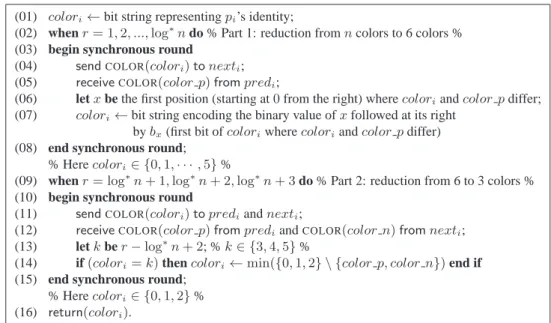
(01) colori← bit string representing pi’s identity;
(02) when r= 1, 2, ..., log∗n do % Part 1: reduction from n colors to 6 colors % (03) begin synchronous round
(04) sendCOLOR(colori) to nexti; (05) receiveCOLOR(color p) from predi;
(06) let x be the first position (starting at0 from the right) where coloriand color p differ; (07) colori← bit string encoding the binary value of x followed at its right
by bx(first bit of coloriwhere coloriand color p differ) (08) end synchronous round;
% Here colori∈ {0, 1, · · · , 5} %
(09) when r= log∗n+ 1, log∗n+ 2, log∗n+ 3 do % Part 2: reduction from 6 to 3 colors % (10) begin synchronous round
(11) sendCOLOR(colori) to prediand nexti;
(12) receiveCOLOR(color p) from prediandCOLOR(color n) from nexti;
(13) let k be r− log∗n+ 2; % k ∈ {3, 4, 5} %
(14) if(colori= k) then colori← min({0, 1, 2} \ {color p, color n}) end if (15) end synchronous round;
% Here colori∈ {0, 1, 2} % (16) return(colori).
Description of the algorithm Let r denote the current round number. Initialized to1, it takes then the
successive values 2, 3, etc. It is global variable provided by the synchronous system, which can be read by all processes.
Each process pi first defines its current color as the bit string representing its identity (line 01).
As already indicated, it is assumed that each identity can be coded on log n bits. Then pi executes
synchronous rounds until it obtains its final color (line 16). The total number of rounds that are executed islog∗n+ 3, which decompose into two parts.
The firstlog∗n rounds (lines 03-08) allow each process pito compute a color in the set{0, 1, · · · , 5}.
Considering a round r, let k be an upper bound on the number of different colors at the beginning of round k, and m be the smallest integer such that k ≤ 2m. Hence, at round r, the color of a process is
coded on m bits. After a send/receive communication step (lines 04-05), a process picompares its color
with the one it has received form its predecessor (color p), and computes (starting at0 from the right),
the bit position x where they differ (line 06). Assuming for example that k = 28
(hence m = 8), let colori = 10011001 and color p = 11011101; we have then x = 2. Then (line 07), pi defines its new
color as the bit sequence whose prefix is the binary encoding of x onlog m bits (010 in our example)
and suffix is the first bit of its current color where both colors differ, namely bx (bx = b2 = 0 in the
example). Hence, its new color is010bx= 0100.
Let consider two neighbor processes during a round r. If they have the same value for x, due to the bit suffix they use to obtain their new color, they necessarily obtain different new colors. If they have different values for x, they trivially have different new colors.
It is easy to see (from the computation of the position x –which defines the prefix of the new color–, and the value of the bit bx –which defines the suffix of the new color–), that the round r reduces the
number of colors from k to at most2⌈log k⌉ ≤ 2m. It is shown in [4] that, after at most log∗n rounds,
the binary encoding of a color requires only three bits, where the suffix bxis0 or 1, and the prefix is 00,
10, or 01. Hence, only six color values are possible 000, 100, 010, 001, 101, and 011.
The second part of this synchronous algorithm consists of three additional rounds, each round elim-inating one of the colors in{3, 4, 5} (lines 10-15). More precisely, each process first exchanges its color
with its two neighbors. Due to the previouslog∗n rounds, these three colors are different. Hence, if its
color is3, pi selects any color in{0, 1, 2} not owned by its neighbors. This is then repeated twice to
eliminate the colors4 and 5.
This algorithm has two main features. The first is the clever and original way a new color is com-puted. The second is its asymptotical time-optimality (log∗n+ 3 synchronous rounds), which follows
from Linial’s result [11]. Proofs of the algorithm correctness and its time complexity can be found in [4, 19].
From a ring to a chain A chain is a sequence where each vertex appears at most once (a ring that has been cut). Hence, each non-singleton chain has two processes that define its ends.
At line 05, the process that has no predecessor cannot compare its current color with another color. It simply does as if it has a (fictitious) predecessor whose color is different from its initial color, and executes normally the algorithm. As an example, if pi (whose initial color is 100101) is the process
without predecessor, it considers a fictitious predecessor whose color is the same as its color except for its first bit (starting from the right), i.e., the color100100). It follows from the algorithm that after the
first round, piobtains the color01 (which will never change thereafter).
Finally, at line 12, an end process defines the color of its “missing neighbor” as being the “no-color” denoted−1.
4
Extending Cole-Vishkin’s Algorithm to Asynchronous Starting Times
This section presents an extension of CV86 for reliable synchronous systems, which allows processes to start at different rounds: the round at which a process starts depends only on it. (Due to the synchrony assumption, when a process starts, it does it at the beginning of a round, and runs then synchronously.)
4.1 Asynchronous starting times and unit-segment
Ring structure and starting time of a process Let sti denote the round number at which process
pi wakes up and starts participating in the algorithm. There is no requirement on the round at which a
process must start the algorithm.
Notion of a unit-segment A unit-segment is a maximal sequence of consecutive processes (with re-spect to the ring) pa, pnexta,· · · , ppredz, pz, that started the algorithm at the same round number.
Hence, a segment is identified by a starting time (round number), and any two contiguous unit-segments are necessarily associated with distinct starting times. It follows that, from an omniscient observer’s point of view, and at any time, the ring can be decomposed into a set of unit-segments, some of these unit-segments being contiguous, while others are separated by processes that have not yet started (or will never start, due to an initial crash). In the particular case where all processes start simultaneously, the ring is composed of a single unit-segment.
4.2 A coloring algorithm with asynchronous starting times
This section presents an extension of CV86 (called AST-CV), which allows processes to start at different rounds. The algorithm is made up of four parts. It requires a process to execute∆ = log∗n+ 6 rounds
(hence it keeps the locality property of CV86). The algorithm is decomposed into four parts.
Starting round of the algorithm The underlying synchronous system defines the first round (r = 1)
as being the round at which a process starts (or a set of processes simultaneously start) the algorithm, while no process started the algorithm before. Hence, when this process starts the algorithm, we have
sti= 1. Then, the progress of r is managed by the system synchrony.
Part 1 and Part 2 These parts are described in Figure 2. Considering a unit-segment (identified by a starting time st) they are a simple adaptation of CV86, which considers the behavior of any process pi
belonging to this unit-segment.
A process piexecutes firstlog∗n synchronous rounds. During each round, it sends its current color
to its neighbors, and receives their current colors. Let msg pred= ⊥ if there is no message from predi
(line 04).
At line 05, the value sti allows pi to know if its predecessor belongs to the same unit-segment
(defined by the value sti). If it the case, pi executes CV86. If its predecessor belongs to a different
unit-segment or has not yet started the algorithm, pi considers a fictitious predecessor whose identity
is the same as its own identity, except for the first bit, starting from the right (see the last paragraph of Annex 3.2). Lines 06-10 constitute the core of CV86, which exponentially reduces the bit size represen-tation of coloriat every round, to end up with a color in the set{0, 1, · · · , 5} after log∗n rounds.
Part 2 of AST-CV (lines 13-21) is the same as in CV86. It reduces the set of colors in each unit-segment from at most six to at most three. It then follows from CV86 [4] that, at the end of this part, the processes of the unit-segment identified by sti have obtained a proper color within their unit-segment.
Moreover, afterlog∗n+ 3 rounds, the color obtained by a process will be its final color if this process
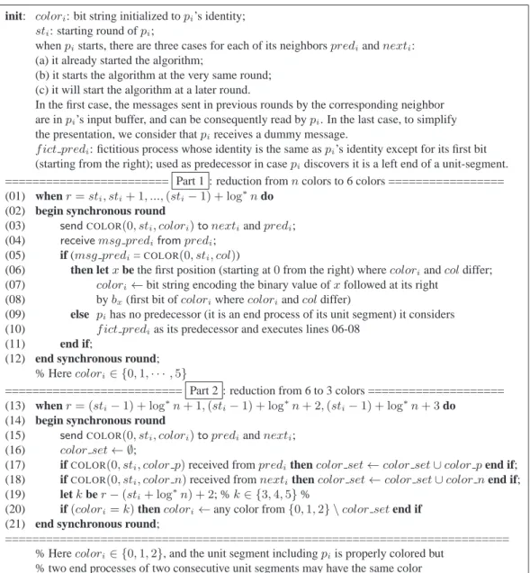
init: colori: bit string initialized to pi’s identity;
sti: starting round of pi;
when pistarts, there are three cases for each of its neighbors prediand nexti: (a) it already started the algorithm;
(b) it starts the algorithm at the very same round; (c) it will start the algorithm at a later round.
In the first case, the messages sent in previous rounds by the corresponding neighbor are in pi’s input buffer, and can be consequently read by pi. In the last case, to simplify the presentation, we consider that pireceives a dummy message.
f ict predi: fictitious process whose identity is the same as pi’s identity except for its first bit (starting from the right); used as predecessor in case pidiscovers it is a left end of a unit-segment. ======================== Part 1 : reduction from n colors to 6 colors ================= (01) when r= sti, sti+ 1, ..., (sti− 1) + log∗n do
(02) begin synchronous round
(03) sendCOLOR(0, sti, colori) to nextiand predi; (04) receive msg predifrom predi;
(05) if (msg predi=COLOR(0, sti, col))
(06) then let x be the first position (starting at0 from the right) where coloriand col differ; (07) colori← bit string encoding the binary value of x followed at its right
(08) by bx(first bit of coloriwhere coloriand col differ)
(09) else pihas no predecessor (it is an end process of its unit segment) it considers (10) f ict predias its predecessor and executes lines 06-08
(11) end if;
(12) end synchronous round; % Here colori∈ {0, 1, · · · , 5}
========================== Part 2 : reduction from 6 to 3 colors ==================== (13) when r= (sti− 1) + log∗n+ 1, (sti− 1) + log∗n+ 2, (sti− 1) + log∗n+ 3 do
(14) begin synchronous round
(15) sendCOLOR(0, sti, colori) to prediand nexti; (16) color set← ∅;
(17) ifCOLOR(0, sti, color p) received from predithen color set← color set ∪ color p end if; (18) ifCOLOR(0, sti, color n) received from nextithen color set← color set ∪ color n end if; (19) let k be r− (sti+ log∗n) + 2; % k ∈ {3, 4, 5} %
(20) if(colori= k) then colori← any color from {0, 1, 2} \ color set end if (21) end synchronous round;
========================================================================== % Here colori∈ {0, 1, 2}, and the unit segment including piis properly colored but
% two end processes of two consecutive unit segments may have the same color Figure 2: Initialization, Part 1, and Part 2, of AST-CV (code for pi)
Message management Let us observe that, as not all processes start at the same round, it is possible that, while executing a round of the synchronous algorithm of Figure 2, a process pireceives a message
COLOR(0, st, −) (with st 6= sti) from its predecessor, or messages COLOR(j, ) (where j ∈ {1, 2, 3},
sent in Parts 3 or 4) from one or both of its neighbors. To simplify and make clearer the presentation, the reception of these messages is not indicated in Figure 2. It is implicitly assumed that, when they are received during a synchronous round, these messages are saved in the local memory of pi(so that they
can be processed later, if needed, at lines 25-28 and line 39 of Figure 3).
Moreover, a process pilearns the starting round of predi (resp., nexti) when it receives for the first
time a messageCOLOR(0, st, −) from predi (resp. nexti). To not overload the presentation, this is left
implicit in the description of the algorithm.
Why Part 3 and Part 4 These parts are described in Figure 3. If pi is a left end, or a right end, or
both, of a unit-segment4, its color at the end of Part 2 is not necessarily its final color. This is due to the
4A process p
fact that Part 1 and Part 2 color the processes in each unit-segment independently from the coloring of its contiguous unit-segments (if any). Hence, it is possible for two contiguous unit-segments to be such that the left end of one (say pi) and the right end of the other (say pj) are such that colori = colorj.
The aim of Part 3 and Part 4 is to solve these coloring conflicts. To this end, each process pimanages
six local variables, denoted colori[j, nbg], where j ∈ {1, 2, 3} and nbg ∈ {predi, nexti}. They are
initialized to−1 (no color).
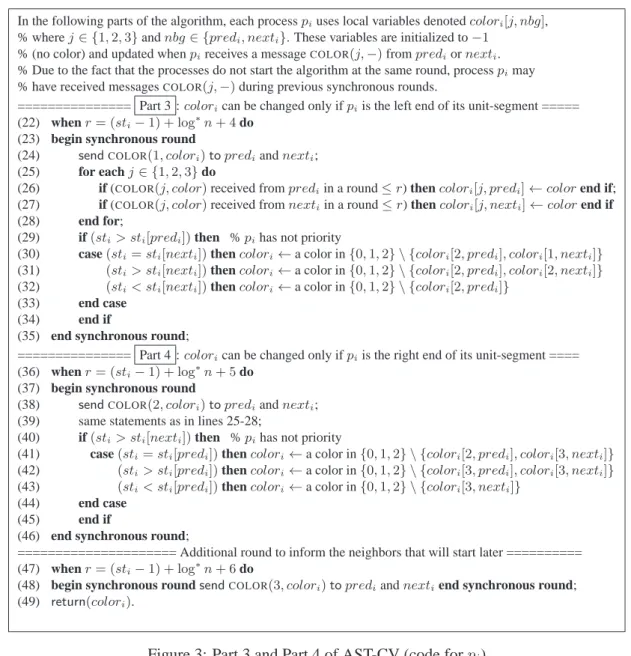
In the following parts of the algorithm, each process piuses local variables denoted colori[j, nbg], % where j∈ {1, 2, 3} and nbg ∈ {predi, nexti}. These variables are initialized to −1
% (no color) and updated when pireceives a messageCOLOR(j, −) from predior nexti. % Due to the fact that the processes do not start the algorithm at the same round, process pimay % have received messagesCOLOR(j, −) during previous synchronous rounds.
=============== Part 3 : colorican be changed only if piis the left end of its unit-segment ===== (22) when r= (sti− 1) + log∗n+ 4 do
(23) begin synchronous round
(24) sendCOLOR(1, colori) to prediand nexti;
(25) for each j∈ {1, 2, 3} do
(26) if (COLOR(j, color) received from prediin a round≤ r) then colori[j, predi] ← color end if; (27) if (COLOR(j, color) received from nextiin a round≤ r) then colori[j, nexti] ← color end if
(28) end for;
(29) if(sti> sti[predi]) then % pihas not priority
(30) case(sti= sti[nexti]) then colori← a color in {0, 1, 2} \ {colori[2, predi], colori[1, nexti]} (31) (sti> sti[nexti]) then colori← a color in {0, 1, 2} \ {colori[2, predi], colori[2, nexti]} (32) (sti< sti[nexti]) then colori← a color in {0, 1, 2} \ {colori[2, predi]}
(33) end case
(34) end if
(35) end synchronous round;
=============== Part 4 : colorican be changed only if piis the right end of its unit-segment ==== (36) when r= (sti− 1) + log∗n+ 5 do
(37) begin synchronous round
(38) sendCOLOR(2, colori) to prediand nexti; (39) same statements as in lines 25-28;
(40) if(sti> sti[nexti]) then % pihas not priority
(41) case(sti= sti[predi]) then colori← a color in {0, 1, 2} \ {colori[2, predi], colori[3, nexti]} (42) (sti> sti[predi]) then colori← a color in {0, 1, 2} \ {colori[3, predi], colori[3, nexti]} (43) (sti< sti[predi]) then colori← a color in {0, 1, 2} \ {colori[3, nexti]}
(44) end case
(45) end if
(46) end synchronous round;
===================== Additional round to inform the neighbors that will start later ========== (47) when r= (sti− 1) + log∗n+ 6 do
(48) begin synchronous round sendCOLOR(3, colori) to prediand nextiend synchronous round; (49) return(colori).
Figure 3: Part 3 and Part 4 of AST-CV (code for pi)
Solving the conflict between neighbors belonging to contiguous unit-segments A natural idea to solve such a coloring conflict between two neighbor processes belonging to contiguous unit-segments, consists in giving “priority” to the unit-segment whose starting time is the first.
Let sti[predi] (resp., sti[nexti]) be the knowledge of pion the starting time of its left (resp., right)
neighbor. If predi has not yet started let sti[predi] = +∞ (and similarly for nexti). Thanks to this
information, pi knows if it is at the left (resp., right) end of a unit-segment: this is the case if sti 6=
sti[predi] (resp., if sti 6= sti[nexti]). Moreover, if pi is a left (resp., right) end of a unit-segment, it
required to change its color to ensure it differs from the color of its neighbor belonging to the priority contiguous unit-segment.
The tricky cases are the ones of the unit-segments composed of either a single process p or two processes paand pb. This is because, in these cases, it can be required that p (possibly twice, once as
right end, and once as left end of its unit-segment), or once paand once pb (in the case of a 2-process
unit-segment), be forced to change the color they obtained at the end of Part 2, to obtain a final color consistent with respect to their neighbors in contiguous unit-segments. To prevent inconsistencies from occurring, it is required that (in addition to the previous priority rule) (a) first a left end process of a segment modifies its color with respect to its predecessor neighbor (which belongs to its left unit-segment), and (b) only then a right end process of a unit-segment modifies its color if needed5.
Summary statement Let us consider a process pi.
• If piis inside a unit-segment (i.e., sti = sti[predi] = sti[nexti] ),
or is the left end of a unit-segment and predibegan after it (i.e., sti < sti[predi]),
or is the right end of a unit-segment and nextibegan after it (i.e., sti< sti[nexti] ),
then the color it obtained at the end of Part 2 is its final color.
• If pi is the left end of a unit-segment and predi began before pi (i.e., sti > sti[predi]), then pi
may be forced to change its color. This is done in Part 3. The color piobtains at the end of Part
3 will be its final color, if it is not also the right end of its unit-segment and nextibegan before it
(i.e., sti > sti[nexti]).
• This case is similar to the previous one. If pi is the right end of a unit-segment and nexti began
before it (i.e., sti > sti[nexti]), pimay be forced to change its color to have a final color different
from the one of nexti. This is done in Part 4.
As a process, that is neither the left end, nor the right end of a unit-segment, obtains its final color at the end of Part 2, it follows that, during Part 3 and Part 4, such a process only needs to execute the sending of messages COLOR(j, −), j ∈ {1, 2, 3} at lines 24, 38, and 48 (the other statements cannot change its color).
Part 3 This part is composed of a single round (lines 22-35). A process pisends first to its neighbors
a messageCOLOR(1, c) carrying the color c it has obtained at the end of Part 2. Then, according to the messages it received from them up to the current round, pi updates its local variables colori[j, predi]
and colori[j, nexti] (lines 25-28).
Part 4 This part, composed of a single round (lines 36-46), is similar to the previous one. Due to the predicate of line 40, the lines 41-44 are executed only if pi is the right end of its unit segment. Their
meaning is similar to the one of lines 30-33.
Finally, pisends (line 48) to its two neighbors the messageCOLOR(3, colori) to inform them of its
last color, in case it was modified in Part 4.
An example Let us consider that pℓ, pa, pb, and prare four consecutive processes such that (i) stℓ =
10, and pℓobtained the final color1, (ii) str = 12, and probtained the final color2, and (iii) paand pb
starts the algorithm at time15. Hence, paand pb define a unit-segment, whose starting time is greater
than the one of both pℓ and pr. Hence, the unit segment composed of paand pb has not priority with
respect to its two contiguous unit-segments.
5
This specific order is only a design choice. The other order (first right end process, then left end process) could have been chosen. What is important is that the processes obey the same order. Differently, being defined from starting times and favoring the oldest starting times, the previous priority order is not a design choice in the sense that the other choice would not work (as not all processes can be participating in the algorithm).
Let us suppose that after having executed Part 1 and Part 2, paobtains the color1, while pb obtains
the color2, i.e., each obtains a color different from its neighbor in the same unit-segment, but this color
is the same as the one of its other neighbor (which belongs to a contiguous “older” unit-segment). As pa is the left end of its unit-segment and started after preda (=pℓ), it received the message
COLOR(2, 1) from pℓ(line 26), and consequently obtains colora[2, preda] = 1. Moreover, as pais in the
same unit-segment as pb, it receives the messageCOLOR(1, 2) from pband obtains colora[1, nexta] = 2
(line 27). Then process pa executes lines 29-30, and obtains the color0 (this is because {0, 1, 2} \
{colora[2, preda], colora[1, nexta]} = {0, 1, 2} \ {1, 2} = {0}).
As stb = sta, pb does not execute lines 30-33, but received the message COLOR(2, 0) from pa
at line 39, and we have consequently colorb[2, predb] = 0. It also received COLOR(3, 2) from pr
(line 39), and we have colorb[3, nextb] = 2. Process pb then executes lines 40-41. As {0, 1, 2} \
{colorb[2, predb], colorb[3, nextb]} = {0, 1, 2} \ {0, 2} = {1}, it obtains its final color 1.
It follows that the final colors of the sequence of the four processes pℓ, pa, pb, and pris1, 0, 1, 2.
4.3 Properties of the algorithm
Due to its construction from CV86, AST-CV inherits its two most important properties, namely locality and determinism.
• In CV86, the locality property states that a process obtains its final color after log∗n+ 3 rounds.
In AST-CV, it obtains itlog∗n+ 6 rounds after it starting round.
• In CV86, the determinism property states that the final color of a process depends only of the
identities of the consecutive processes which are itslog∗n+ 3 predecessors on the ring. In
AST-CV, its final color depends only of the starting times and the identities of the consecutive processes which are itslog∗n+ 6 predecessors on the ring.
4.4 Proof of the algorithm
Definition 1. The final color of a process is the color it returns at line 49.
Lemma 1. Let pibe a process which wakes up at time sti. After pi has executed the round(sti− 1) +
log∗n+ 3 (Part 1 of Figure 2), no two neighbors of its unit-segment have the same color. Moreover, their colors are in the set{0, 1, 2}.
Proof The proof follows from the observation that, when considering the processes of a unit-segment, Part 1 and Part 2 of Figure 2 boils down to CV86, from which the lemma follows. ✷Lemma 1
Lemma 2. Let pi be a process that wakes up. If pi is neither the left end, nor the right end, of its
unit-segment, its final color is the color it obtains at the end of Part2.
Proof If pi is neither the left end nor the right end of its unit-segment we have sti = sti[predi] =
sti[nexti]. The lemma follows then directly from the predicates of lines 29 and 40. ✷Lemma 2
Lemma 3. If piwakes up, its final color belongs to{0, 1, 2}.
Proof The proof follows from Lemma 1 and the fact, whatever the lines 30-32 and 41-43 executed by a process pi(if some are ever executed), any of them restricts the new color to belong to the set{0, 1, 2}.
✷Lemma 3
Lemma 4. Let us assume that both pi and pj wake up, where pj is pnexti. If pi and pj belong to the
Proof The proof is a case analysis. There are four cases, namely:
Case (a): piis not the left end and pjis not the right end of their unit-segment,
Case (b): piis not the left end and pjis the right end of their unit-segment,
Case (c): piis the left end and pjis not the right end of their unit-segment,
Case (d): piis the left end and pjis the right end of their unit-segment.
Case (a): pi is not the left end and pj is not the right end of their unit segment. In this case, it follows
from Lemma 1 and Lemma 2 that the final color of piand the final color of pjare different.
Case (b): piis not the left end and pj is the right end of their unit-segment. Then, by Lemma 2, the final
color of piis the value of coloriat the end of Part 2 (round(sti− 1) + log∗n+ 3). By the algorithm, pj
does not change its color at round(sti− 1) + log∗n+ 4 (predicate of line 29 where sti = sti[predi]),
but may change it during round(sti− 1) + log∗n+ 5 (Part 5). There are two sub-cases.
• stj < stj[nextj]. In this case the predicate of line 40 is false, and pj does not modify colorj. It
then follows that both pi and pj keep the color they obtained at the end of Part 2. By Lemma 1,
these colors are different.
• stj > stj[nextj]. In this case, pj executes the update of line 41, where the color assigned to
colorj remains different from colori(which was received during a previous round and saved in its
local variable colorj[2, predj]).
Case (c): pi is the left end and pj is not the right end of their unit-segment. By Lemma 2, pj does not
change its color after Part 2 (round(sti− 1) + log∗n+ 3). There are two cases.
• sti < sti[predi]. It follows from the predicate of line 29 that pi does not change its color during
Part 3. As sti= stj, the predicate of line 40 is false, and pidoes not change its color in Part 4. It
then follow from Lemma 1 that piand pjhave different final colors.
• sti > sti[predi]. As pi and pj are in the same unit-segment, pi receives COLOR(1, colorj) at
line 27 during the round(sti− 1) + log∗n+ 4 (Part 3), and saves this value in its local variable
colori[1, nexti]. Then, due to the predicates of lines 29 and 30, pi changes its color at line 30
during the round(sti− 1) + log∗n+ 4 (Part 3), and this color is different from the final color of
pj. Finally, as sti = stj, the predicate of line 40 is not satisfied, and pi does not update colori
during the round(sti− 1) + log∗n+ 5 (Part 4). It then follows from that piand pj have different
final colors.
Case (d): piis the left end and pjis the right end of their unit-segment. There are four cases.
• sti < sti[predi] and stj < stj[nextj]. In this case, piand pjdo not change their color after round
(sti− 1) + log∗n+ 3. Hence, by Lemma 1, they will have different final colors.
• sti < sti[predi] and stj > stj[nextj]. In this case, when evaluated by pi, the predicates of
lines 29 and 40 (we have then sti = sti[nexti] = stj) are false. Hence, pi does not change its
color after round(sti− 1) + log∗n+ 3. This case is similar to the second sub-case of Case (b).
• sti > sti[predi] and stj < stj[nextj]. In this case pjdoes not change its color after Part 2 (round
(stj− 1) + log∗n+ 3). This case is similar to the second sub-case of Case (c).
• sti > sti[predi] and stj > stj[nextj]. Due to the predicates of lines 29 and 30, pi changes its
color at line 30 during round (sti− 1) + log∗n+ 4 (Part 3). Moreover, as sti = stj, it does
not change its color in Part 4. Hence, its final color is the one obtained at line 30. Differently, as
stj > stj[nextj] and stj = sti, pj updates its color at line 41 during round(stj− 1) + log∗n+ 5
(Part 4), where it obtains a color different from colori (final color of pi received at line 38 and
✷Lemma 4
Lemma 5. Let us assume that both pi and pj wake up, where pj is pnexti. If pi and pj are not in the
same unit-segment and sti > stj, their final colors are different.
Proof The processes pi and pj are neighbors but belong to different unit-segments. As stj < sti and
all processes gets their final color after the same constant number of round after they wake up, pj gets
its final color before pi. The proof considers the following two possible cases: Case (a): pi is not a left
end of its unit segment, and Case (b) piis a left end of its unit segment.
Case (a): pi is not a left end of its unit segment. In this case, it follows from the predicate of line 29
that pidoes not change its color during Part 3, and from the predicates of lines 40 and 41 (Part 4), that
pi updates its color at line 41. As pj woke up before pi, pi received the messageCOLOR(3, col) sent at
line 48 by pjduring its round(stj− 1) + log∗n+ 6. This message was received by piat the latest while
it executes its round(sti− 1)i + log∗n+ 5. Moreover, col is then the final color of pj. It follows that,
when it executes its round(sti− 1) + log∗n+ 5, piis such that colori[3, nexti] = col. Consequently,
at line 41, piadopts a final color different from the final color of pj.
Case (b): piis a left end of its unit segment. We consider two sub-cases.
• sti < sti[predi]. In this case, it follows from the predicate of line 29 that pi does not change
its color during Part 3. Differently, due to the predicates of lines 40 and 43, it updates colori at
line 43. Moreover, as sti> stj, pireceived from pj the messageCOLOR(3, col) (where col is the
final color of pj) at a round≤ (sti− 1) + log∗n+ 5, and saved col in colori[3, nexti]. It then
follows that, when piexecutes line 43, it assigns to coloria value different from the final color of
pj.
• sti > sti[predi]. In this case, it follows from the predicates of lines 29 and 31 that piupdates its
color at line 31 (Part 3), and from the predicates of lines 40 and 42 that pi updates again its color
at line 42 (Part 4).
As pj woke up before pi, pi received the message COLOR(3, col) from pj before (or at) round
(sti− 1) + log∗n+ 5 (Part 4), and col is the final color of pj. It follows that, when pi updates
its color at line 42, we have colori[3, nexti] = col. Consequently, the final color of piis different
from the final color of its neighbor pj.
✷Lemma 5
Lemma 6. Let us assume that both pi and pj wake up, where pj is pnexti. If pi and pj are not in the
same unit-segment and stj > sti, their final colors are different.
Proof By assumption, pi and pjare neighbors, but belong to different unit-segments. As stj > stiand
all processes execute the same number of rounds after they woke up (log∗n+6), p
ireturns its final color
(line 49) before pj. As for Lemma 4, the proof of the lemma considers four cases, namely
Case (a): piis not the left end of its unit-segment and pj is not the right end of its unit-segment,
Case (b): piis not the left end of its unit-segment and pj is the right end of its unit-segment,
Case (c): piis the left end of its unit-segment and pj is not the right end of its unit-segment,
Case (d): piis the left end of its unit-segment and pj is the right end of its unit-segment.
Case (a): pi is not the left end of its unit-segment and pj is not the right end of its unit segment. As pi
is not the left end of its unit segment, it follows from the predicate of line 29 that it does not update its color in Part 3. As sti< stj = sti[nexti], it follows from the predicate of line 40 that pidoes not update
As far as pj is concerned, we have the following. As stj > sti and pj is not the right end of its
unit-segment, the predicates of lines 29 and 30 direct pj to update its color at line 30 (Part 3). Moreover,
as pj is not the right end of its unit-segment, the predicate of line 40 is not satisfied and pj does not
change its color in Part 4.
As piwoke up before pj, pj received the messageCOLOR(2, col) from piat a round≤ (stj− 1) +
log∗n+ 4, and col is the final color of pi. It follows that when pjexecutes line 30, it assigns to colorj a
color different from the final color of pi.
Case (b): pi is not the left end of its unit-segment and pj is the right end of its unit-segment. As pi is
not the left end of its unit-segment and sti < stj, it follows that the predicate of line 29 is not satisfied
when evaluated by pi. Similarly, as sti < sti[nexti] = stj, the predicate of line 40 is not satisfied either.
Consequently, pi does not modify its color in Part 3 or Part 4. Let cl i be this color.
As piwakes up before pj, pj has received the messageCOLOR(2, cl i) sent by piat the latest
dur-ing its round (stj − 1) + log∗n+ 4 (Part 3). Hence, at the end of round (stj − 1) + log∗n+ 4,
colorj[2, predj] = cl i. Moreover, pjreceived the messageCOLOR(3, cl i) at the latest during its round
(stj− 1) + log∗n+ 5, and saved it in colorj[3, predj] = cl i. It then follows that, whatever the update
of colorj done by pj at any line of Part 3 (lines 30-32) or Part 4 (lines 41-43), the final color of pj will
be different from the final color of pi.
Case (c): piis the left end of its unit-segment and pj is not the right end of its unit-segment.
As pi is the left end of its unit-segment, it may be forced to update its color (at line 32 because
stj > sti) if the predicate of line 29 is satisfied (Part 3). But as stj > sti, the predicate of line 40 cannot
be satisfied (Part 4). Hence, both the messagesCOLOR(2, cl i) andCOLOR(3, cl i) sent by piat lines 38
and 48 carry its final color.
As stj > sti, pj receivedCOLOR(2, cl i) at the latest during its round (stj− 1) + log∗n+ 4, and
COLOR(3, cl i) at the latest during its round (stj− 1) + log∗n+ 5. It follows that, whatever the update
of colorj done by pjwhen it executes Part 3 or Part 4, its final color will be different from cl i.
Case (d): piis the left end of its unit-segment and pj is the right end of its unit-segment.
As indicated in the previous case, pi (left end of its unit-segment) may change its color due the
predicates of lines 29 and 32 when it executes its round(sti− 1) + log∗n+ 4 (Part 3), but (as sti < stj)
it will not change it in Part 4. We consider two cases. Let cl i be the final color of pi.
• stj > stj[nextj]. In this case, As stj > sti the predicate of line 29 is satisfied, and pj updates
its color at line 31 when it executes its round (stj − 1) + log∗n+ 4 (Part 3). Similarly, as
stj > stj[nextj], pjupdates its color at line 42 when it executes its round(stj− 1) + log∗n+ 4
(Part 4). As pj woke up after pi, it receivedCOLOR(2, cl i) from pi at the latest when it executes
its round(stj− 1) + log∗n+ 4 (Part 3), and receivedCOLOR(3, cl i) at the latest when it executes
its round(stj− 1) + log∗n+ 5 (Part 4). It follows that, whatever (if any) an update of colorj
done at any of the lines 30-32 and 41-43, the final color of pj will be different from the one of pi.
• stj < stj[nextj]. In this case, pj may update its color at line 32 while executing its round
stj + log∗n+ 4 (Part 3). As sti < stj, pj receives the message COLOR(2, cl i) from pi at the
latest during its round (stj − 1) + log∗n+ 4 (cl i is the final color of pi), and consequently
colorj[2, predj] = cl i at round (stj − 1) + log∗n+ 4. Hence, when it executes line 32, pj
updates colorj to a color different from cl i. Let us finally observe that, as stj < stj[nextj],
the predicate of line 40 (Part 4) is not satisfied, and consequently pj does not modify colorj at
lines 41-43, which completes the proof of the lemma.
✷Lemma 6
Theorem 1. If pi and pj wake up and are neighbors, their final colors are different and in the set
Proof The proof follows from the Lemma 3, Lemma 4, Lemma 5, and Lemma 6. ✷T heorem 1
5
From Asynchronous Starting Times to Wait-freedom
Considering the two-component-based model introduced in Section 2, this section presents the WLC (Wait-free Local Coloring) algorithm which colors the processes of a ring in at most three colors. This algorithm relies on two consecutive stages executed independently by each computing process. The first stage is a communication stage during which, whatever its starting time, each process obtains enough information to locally execute its second stage, which is communication-free. As in Section 4, a
unit-segment is a maximal sequence of consecutive processes that started the algorithm at the same time (i.e.,
as the same clock tick as defined by the underlying synchronous communication component).
Before presenting the algorithm WLC, we need a solvability notion that incorporates asynchrony and failures that are present inDECOU PLED. An algorithm wait-free solves m-coloring if for each of
its executions:
• (Validity. The final color of any process is in {0, . . . , m − 1}.
• Agreement. The final colors (if any) of any two neighbor nodes in the graph are different. • Termination. In every infinite extension of the execution, all processes decide a final color.
5.1 On the communication side
A ring structure for the synchronous communication network The neighbors of a node ndi (or
process pi with a slight abuse of language) are denoted as before, namely prediand nexti.
On the side of the communication nodes While each input buffer iniis initially empty, each output
buffer outiis initialized tohi, +∞, ⊥i. When a process starts its participation in the algorithm, it writes
the pair hi, sti, idii in outi, where sti is its starting time (as defined by the current tick of the clock
governing the progress of the underlying communication component), and idiis its identity.
As already described, at every clock tick (underlying communication step), ndi first receives two
messages (one from each neighbor), and reads the local buffer outi. Then, it packs the content of these
two messages and the content of outi (which can behi, +∞, ⊥i if pi has not yet started) into a single
message, sends it to its two neighbors, and writes it in ini6.
5.2 Wait-free algorithm: first a communication stage
Let pi be a process that starts the algorithm at time sti = t. As previously indicated, this means that,
at time t (clock tick defined by the communication component), pi writeshi, t, idii in its output buffer
outi. Then pi waits until time t+ ∆ where ∆ = log∗n+ 5. (7). At the end of this waiting period, and
as far piis concerned, the “dices are cast”. No more physical communication will be necessary. As we
are about to see, pi obtained enough information to compute alone its color: the rest of the algorithm
executed by piis purely local (see below). This feature, and the fact that the starting time of a process
depends only on it, makes the algorithm wait-free.
It follows from the underlying communication component that, at time t+ ∆, pi has received an
information (i.e., a triplethj, st, idji) from all the processes at distance at most ∆ of it. If st = t, pi
knows that pj started the algorithm at the same time as it. If st < t (resp., st > t), pi knows that pj
6
Full-information behavior of a node.
7Being asynchronous, the waiting of p
iduring an arbitrary long (but finite) period does not modify its allowed behavior. Let us observe that a crash is nothing other than an infinite waiting period.
started the algorithm before (resp., after) it. (If st= +∞ –we have then idj = ⊥– and pj is at distance
d from it, piknows that pj did not start the algorithm before the clock tick t+ ∆ − d.)
5.3 Wait-free algorithm: then a local simulation stage of AST-CV
At the end of its waiting period, pi has information (pairs composed of a starting time and a process
identity, possibly equal to+∞ and ⊥, respectively) of all the processes at distance ∆ = log∗n+ 5 from
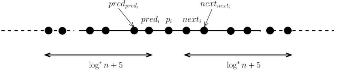
it (Figure 4.) More precisely, for each process pj at distance at most∆ from it, pi knows whether pj
started before it (stj < sti), at the same as it (stj = sti), or after it (stj > sti).
pi
predi nexti
nextnexti
predpredi
log∗n + 5 log∗n + 5
Figure 4: What is know by piat time sti+ ∆
Simulation of AST-CV It follows from the previous observation that, after its waiting period, pi has
all the inputs (starting times and process identities) needed to simulate AST-CV and compute its final color, be it inside a unit-segment, the left end of a unit-segment, the right end of a unit-segment, or both ends of a unit-segment. More precisely, this simulation is as follows. Process pi sequentially simulates
the following∆ rounds of AST-CV:
• A first round involving the 2∆ + 1 processes at distance ≤ ∆ from itself, followed by
• A second round involving the 2∆ − 1 processes at distance ≤ ∆ − 1 from itself, etc., followed by • A (∆ − x + 1)th round involving the processes at distance ≤ x from itself, etc., followed by • A ∆th round involving predi, nextiand itself.
It then follows from the determinism and locality properties of AST-CV that, after it has simulated the previous rounds, piobtained its final color.
Remark Let us observe that the crash of a process pk has no impact on the termination and the
cor-rectness of the coloring of the other processes. This follows from the locality property of AST-CV. If the distance between pi and pk is more than∆ = log∗n+ 5, pk cannot impact the color obtained by
pi. If the distance between pi and pk is less or equal to∆ = log∗n+ 5, the input information of pk
(identity and starting time) is needed by pionly if pkstarted the algorithm before or at same time as pi.
But, in this case, due to the waiting period of pi’s communication stage, this information is known by
pi. Process piconsiders then pkas competing for a color, be it crashed or not.
Optimality of WLC Each process in WLC performs (asynchronously) O(log∗n) rounds of
commu-nication. This number of rounds is asymptotically optimal as
1. Ω(log∗n) is a lower bound on the number of time units (communication rounds) needed to color
the nodes of a ring, with at most three colors [11] inLOCAL.
6
Conclusion
Contributions This paper has two main contributions. The first is a distributed computing model where communication and processing are decoupled. More precisely, asynchronous crash-prone pro-cesses run on top of a reliable synchronous network. This model is weaker than the synchronous model (on the process side) and stronger than the asynchronous crash-prone model (on the communication side). A main advantage of this model is to provide us with a single framework where both the words “locality” [11] and “wait-freedom” [9] have a meaning. As these words capture fundamental concepts of distributed computing, the proposed model establishes a bridge linking synchronous reliable systems (for the communication side) and asynchronous crash-prone systems (for the computing process side), which reconciles these two worlds.
The second contribution of the paper is an illustration of the benefit of the proposed model, namely, an optimal ring-coloring wait-free algorithm. This algorithm uses as a subroutine a generalization of Cole and Vishkin’s well-known algorithm [4], and benefits from its locality property, namely, a process needs to obtain initial formation from processes at distance at most O(log∗n) of it. As far as we know,
this is the first wait-free coloring algorithm, which colors a process ring with at most three colors. Towards a global view As already explained, a main difference in the DECOU PLED model is
that after d rounds of communication, a process collects the initial inputs of only a subgraph of its
d-neighborhood. Despite this uncertainty, the paper has presented a way to marry locality and
wait-freedom, as far as distributed graph coloring is concerned. The keys of this marriage were (a) the decoupling of (reliable synchronous) communication and (asynchronous crash-prone) processing, and (b) the design of an intermediary synchronous coloring algorithm (AST-CV), where the processes are reliable, proceed synchronously, but are not required to start at the very same round. This introduces a first type of asynchrony among the processes. As we have seen, the heart of this algorithm lies in the consistent coloring of the border vertices of subgraphs which started at different times (segment units).
It would be interesting to see if this methodology could apply to other local coloring algorithms, or even, more ambitiously, to other distributed graph problems which are locally solvable in theLOCAL
synchronous model.
Acknowledgments
This work has been partially supported by the French ANR project DISPLEXITY, which is devoted to computability and complexity in distributed computing. The first author was supported in part by UNAM PAPIIT-DGAPA project IA101015. The fourth author was supported in part by UNAM PAPIIT-DGAPA project IN107714.
References
[1] Barenboim L. and Elkin M., Deterministic distributed vertex coloring in polylogarithmic time. Journal of the ACM, 58(5):23, 2011.
[2] Barenboim L. and Elkin M., Distributed graph coloring, fundamental and recent developments, Morgan & Claypool Publishers, 155 pages, 2014.
[3] Barenboim L., Elkin M., and Kuhn F., Distributed (Delta+1)-coloring in linear (in Delta) time. SIAM Journal of Com-puting, 43(1):72-95, 2014.
[4] Cole R. and Vishkin U., Deterministic coin tossing with applications to optimal parallel list ranking. Information and Control, 70(1):32-53, 1986.
[5] Fischer M.J., Lynch N.A., and Paterson M.S., Impossibility of distributed consensus with one faulty process. Journal of the ACM, 32(2):374-382, 1985.
[6] Fraigniaud P., Korman A., and Peleg D., Towards a complexity theory for local distributed computing. Journal of the ACM, 60(5), Article 35, 16 pages, 2013.
[7] Garey M.R. and Johnson D.S., Computers and intractability: a guide to the theory of NP-completeness. W.H. Freeman, New York, 340 pages, 1979.
[8] Goldberg A., Plotkin S, and Shannon G., Parallel symmetry-breaking in sparse graphs. SIAM Journal on Discrete Mathematics, 1(4):434-446, 1988.
[9] Herlihy M.P., Wait-free synchronization. ACM Transactions on Programming Languages and Systems, 13(1):124-149, 1991.
[10] Kuhn F., Moscibroda T., and Wattenhofer R., What cannot be computed locally! Proc. 23rd ACM Symposium on Principles of Distributed Computing (PODC’04), ACM Press, pp. 300-309, 2004.
[11] Linial N., Locality in distributed graph algorithms. SIAM Journal on Computing, 21(1):193-201, 1992.
[12] Loui M. and Abu-Amara H., Memory requirements for agreement among unreliable asynchronous processes. Advances in Computing Research, 4:163-183, JAI Press, 1987.
[13] Lynch N.A., Distributed algorithms. Morgan Kaufmann, 872 pages, 1996.
[14] Naor M. and Stockmeyer L., What can be computed locally? SIAM Journal on Computing, 24(6):1259-1277, 1995. [15] Peleg D., Distributed computing, a locally sensitive approach. SIAM Monographs on Discrete Mathematics and
Appli-cations, 343 pages, 2000 (ISBN 0-89871-464-8).
[16] Raynal M., Fault-tolerant agreement in synchronous message-passing systems. Morgan & Claypool Publishers, 165 pages, 2010 (ISBN 978-1-60845-525-6).
[17] Raynal M., Concurrent programming: algorithms, principles, and foundations. Springer, 530 pages, 2013 (ISBN 978-3-642-32026-2).
[18] Suomela J., Survey of local algorithms. ACM Computing Surveys, 45(2), Article 24, 40 pages, 2013. [19] Wattenhofer R., Principles of distributed computing. ETHZ, 240 pages, 2014.