Statistical Analysis of Corrosion Process along French Coast

HAL Id: hal-01008947

https://hal.archives-ouvertes.fr/hal-01008947

Submitted on 29 Apr 2018

HAL is a multi-disciplinary open access archive for the deposit and dissemination of sci-entific research documents, whether they are pub-lished or not. The documents may come from teaching and research institutions in France or abroad, or from public or private research centers.

L’archive ouverte pluridisciplinaire HAL, est destinée au dépôt et à la diffusion de documents scientifiques de niveau recherche, publiés ou non, émanant des établissements d’enseignement et de recherche français ou étrangers, des laboratoires publics ou privés.

Statistical Analysis of Corrosion Process along French

Coast

Franck Schoefs, Jérôme Boéro, Bruno Capra, R. Melchers

To cite this version:

Franck Schoefs, Jérôme Boéro, Bruno Capra, R. Melchers. Statistical Analysis of Corrosion Process along French Coast. ICOSSAR’09, 2009, Osaka, Japan. �hal-01008947�

1 INTRODUCTION

Steel structures in sea or estuary area are subjected to corrosion process. The phenomenon is very com-plex due to the nature of the environment and mate-rial, and the type of the structure. This phenomenon needs to be characterized and modeled for structural analysis which accounts for the loss of thickness. Moreover, due to the randomness of the corrosion process, probabilistic models are needed for struc-tural reliability. Ultrasonic residual measurements allow determining profiles of loss of thickness, iden-tifying the areas which are the most affected by cor-rosion and stating the assumptions for modeling the random corrosion process. Several inspection cam-paigns have been performed during the three last decades in some French harbours. Thus a great number of ultrasonic residual measurements are now available for structures in various environments. The protocol is recommended by the CETMEF (French Center for Maritime and Fluvial Technical Studies :Engineering centre of the French Ministry of Public Works): at a given level, this protocol suggest to perform three geometrical measurements at a given location to assess the loss of thickness as the average of these three readings. Generally, the amount of da-ta is more than 1000 per structure and allows per-forming a statistical analysis of the spatial distribu-tion of the loss of thickness according to the different areas (mainly tidal and immersion areas).

Moreover environmental parameters (temperature, PH, oxygen, salinity, conductivity, nutrients) have been measured since a decade and are available.

This study began within the MEDACHS frame-work (Marine Environment Damage to Atlantic Coast Historical and transport works or Structures-Interreg IIIB Project funded by EC 2005-2007) and is performed now in the GEROM framework (Risk management of French harbor structures: stakes, current practices and needs – Experience feedback of owners). The steel structures are sheet-piles, on-pile and on-sheet-on-pile wharves. This paper focuses on sheet-piles seawalls and coffer-dams. More than 30 000 data are available: they correspond to meas-urements in 4 harbours and concern more than 20 quays. This paper focuses on the spatial dependence of the corrosion process and we present only results of three of them where the distance between data is small (0.20 m horizontally and 0.10 m vertically).

In the first part, the paper presents the data availa-ble to study the spatio(-temporal) fields of corrosion for steel sheet-piles.

The second part presents the geo-statistical model-ing of the spatial variability of the steel sheet piles corrosion; and more particularly the study of the sta-tionarity of the process of corrosion according to the length and the depth along three marine structures. Finally, a first level of stochastic modeling is sug-gested.

Statistical analysis of corrosion process along French coasts

F. Schoefs

GeM, UMR CNRS 6183, Nantes Atlantic University, Nantes, France

J. Boéro & B. Capra

OXAND S.A., Avon, France

R. Melchers

Center of Infrastructure Performance and Reliability, The University of Newcastle, Australia

Modeling of corrosion for steel structures in sea or estuary area is still a great challenge in view to analyze their safety and optimize their maintenance. Several inspection campaigns have been performed during the three last decades in some French harbours. Thus a great number of ultrasonic residual measurements are now available for structures in various environments. This information allows to perform a statistical analysis in view to best understand and model the distribution of loss of matter on those structures according to different areas (mainly tidal and immersion areas). Results confirm that the loss of thickness is higher at the interface between the tidal area and immersion area. An analysis of the spatial process is performed: stationarity is analyzed on three marine structures where the amount of data is significant. Finally, a first level of spatial dependent corrosion modeling of steel in marine environment is suggested.

2 CORROSION DATABASE

2.1 Corrosion measurements

Corrosion of steel structures is classically assessed by ultrasonic non destructive testing. In France, a protocol is given by the CETMEF and classically used by several companies to perform inspections of coastal steel structures. The CETMEF is part of the French ministry of building. It is devoted to the dif-fusion of knowledge, to provide technical and search studies as well as engineering and expert's re-ports. This protocol consists in performing residual thickness measurements for several heights of the structure using ultrasonic testing. The corrosion products are removed by grinding. By using this technique and considering the harsh conditions for marine inspections, the error on the measurements at a given point on the structure cannot be neglected. Error comes both from the physical measurement (around 0.1 mm) and from the protocol (grinding, link diver-operator, etc.). Thus three measurements are performed on a given location: the three meas-urements are distributed on a circle, with diameter of about 5 cm, every 120° as shown on figure 1. The average of these three readings is considered as the “true” loss of thickness. For on-pile wharves, in view to analyze the corrosion around the pile, meas-urements are performed at several cardinal positions of the pile's section (see figure 1). For on-sheet-pile-wall wharves, they are performed along the length of the wharf around every 10 meters, which is classi-cally the mean distance between two piles for on-pile wharves. Starting from these residual thickness values, and knowing the initial thickness of piles or sheet-piles, we deduce the thickness loss mainly due to corrosion. This protocol involves recommenda-tions only and in some cases, this protocol is not fol-lowed because of the experience of owners or the re-sults of the risk based inspection analysis. That is the case for structures considered in the lat part of the structures where the distance between measurements is closer.

Figure 1. CETMEF protocol: cardinal points for pile (left) and location for sheet pile (right).

2.2 Presentation of the corrosion data-base

Corrosion measurements are collected on two types of marine structures: on-pile wharves and on-sheet pile wharves. Structures are located on the French coasts, i.e. Atlantic, Channel and Mediterranean coasts. In this paper, only corrosion measurements associated to steel sheet piles are presented.

Almost all the studied structures were built be-tween 1955 and 1985. Only three structures are older than 1955 and none is more recent than 1985. The owners began NDT measurements of residual thick-nesses from 1990. Consequently most of the struc-tures are 10 to 40 years old at the inspection time. Figure 2 presents the distribution of the age of the structures at the first, second, third and more inspec-tion times.

Figure 2. Age distribution of the studied structures at inspec-tion time.

Four harbours are considered and called BO, HA, PL, SE. The distribution of the structures within the studied harbours and according to the type of water variation (dock at constant seawater level, wet dock and tidal dock) is presented on figure 3.

Figure 3. Harbours and docks distribution.

Over a total amount of 23 structures, 11 are locat-ed in docks at constant seawater level, 9 in tidal docks and 3 in wet docks. In this last case the water level changes with the same period as the tide but with lower amplitude.

The variation of the seawater level in the various docks is detailed on figure 4.

The tide level corresponds to the range between the HAT (Highest Astronomical Tide) and the (LAT (Lowest Astronomical Tide).

Figure 4. Harbours and docks distribution.

The variation of the height of water is important in tidal docks of BO and HA harbours. The variation is of course weaker in harbours located along the Med-iterranean coast (i.e. PL and SE harbours).

Most of the measurements are made in the im-mersed zone, including the zone of low seawater level and the mud zone. Only the HA harbour began some measurements in the tidal/spray and in the at-mospheric zones. The amount of data according to the studied harbours and for the various exposure zones is detailed on the figure 5.

Figure 5. Distribution of data (loss of thickness) in the various exposure zones.

The structure of the BO harbour was alone the subject of large campaign of measurements: it repre-sents 99 % of all the available measurements.

2.3 Selected structures for spatial variability

assessment: inspection campaign

The study of the spatial variability of corrosion is performed from the data of three structures extracted from the database. This selection is based on the fact that the distance between horizontal or vertical measurements are much weaker than everywhere

else. Consequently, the quantity of information is consequent to perform a spatial analysis of the cor-rosion process.

In the three cases, it is important to remind that these specific campaigns were devoted to the discovery of perforations on steel sheet piles. In the case of the structure HA7d, the control was also started after the observation of accidental acids discharges.The main technical characteristics of these structures are de-tailed in tables 1. Table 2 gives more details con-cerning the type of sheet piles and the auscultation strategy.

Table 1. Characteristics of the selected structures. ______________________________________________ Structure BO1 HA7d HA8b ______________________________________________ Function General General General

cargo cargo cargo Type Cofferdam Seawall Seawall Sheet piles Flat U-sections U-sections Width (m) 0.5 0.5 0.5 Length (m) 758.0 345.0 187.5 Age (Years) 25 28 26 Sea Channel Channel Channel Dock type Tidal Constant Constant

seawater seawater level level Seawater

variation level 9.1 0.6 0.6 _____________________________________________

Table 2. Corrosion measurements strategies of the selected structures.

______________________________________________ Structure BO1 HA7d* HA8b ______________________________________________ Location of measurements

on steel sheet piles - In & out Out-pans pans

Length of the measured

part of the structure (m) 758.0 35.0 123.0 Height of the measured

part of the structure (m) 3.0 9.6 6.1 Number of measurements

following length 5988 71 36 Mean horizontal spacing

between measurements (m) 0.15 to 0.5 3.5 0.2

Number of measurements

following depth 7 13 48 Mean vertical spacing

between measurements (m) 0.5 0.8 0.1 Number of loss thickness

measurements 32238 685 504 Measurements location in

several exposure zones** T, L, I L, I L, I ______________________________________________ Tidal zone ZT

______________________________________________ Number of measurements

following depth 2 - - Number of loss thickness

Measurements 11073 - - Percentage of

the total amount of

measurements _{______________________________________________}34 - - Low seawater zone ZL

______________________________________________ Number of measurements

Number of loss thickness

Measurements 5350 220 24 Percentage of

the total amount of

measurements 17 32 4 ______________________________________________ Immersion zone ZI ______________________________________________ Number of measurements following depth 4 9 46 Number of loss thickness

Measurements 15815 465 480 Percentage of

the total amount of

measurements 49 68 96 _____________________________________________ * Measurements alternatively on in and out-pans of U-shape sheet piling.

** ZT = Tidal zone; ZL = Low seawater zone; ZI = Immersion zone.

2.4 Environment of selected structures

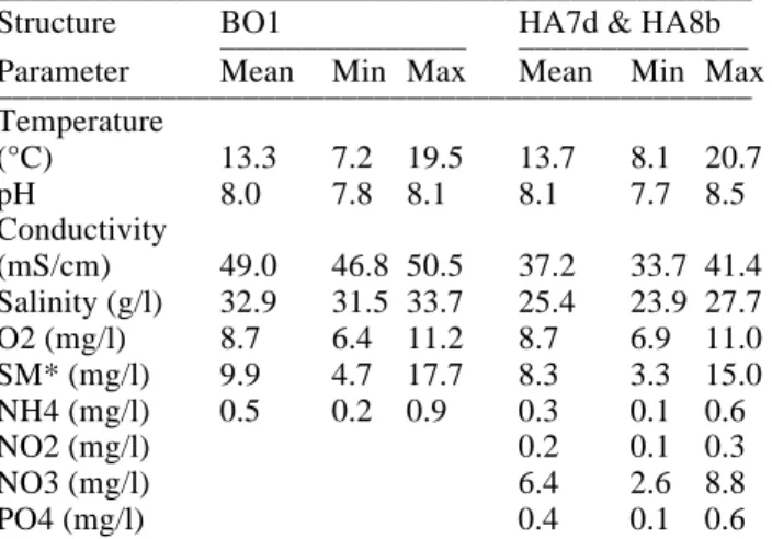
The physico-chemical parameters of seawater near the studied structures are described on table 3. Most of them were measured between 1997 and 2007. Table 3. Mean values and ranges of physico-chemical parame-ters of seawater near the studied structures.

______________________________________________ Structure BO1 _{_______________} HA7d & HA8b _{______________} Parameter Mean Min Max Mean Min Max ______________________________________________ Temperature (°C) 13.3 7.2 19.5 13.7 8.1 20.7 pH 8.0 7.8 8.1 8.1 7.7 8.5 Conductivity (mS/cm) 49.0 46.8 50.5 37.2 33.7 41.4 Salinity (g/l) 32.9 31.5 33.7 25.4 23.9 27.7 O2 (mg/l) 8.7 6.4 11.2 8.7 6.9 11.0 SM* (mg/l) 9.9 4.7 17.7 8.3 3.3 15.0 NH4 (mg/l) 0.5 0.2 0.9 0.3 0.1 0.6 NO2 (mg/l) 0.2 0.1 0.3 NO3 (mg/l) 6.4 2.6 8.8 PO4 (mg/l) 0.4 0.1 0.6 _____________________________________________ * SM = Suspended materials.

The physico-chemical parameters of seawater for the structures HA7d and HA8b are identical because they are located in the same dock.

3 SPATIAL VARIABILITY OF THE CORROSION PROCESS

3.1 Data pre-processing

The loss of thickness on each location is computed by averaging the three readings corresponding to three positions occupied by the ultrasonic transducer inside the required location (see figure 1).

Sometimes, for technical reasons, a single basic measurement is realized in a location. In that case, the loss of thickness which characterizes this

loca-tion was removed from the database because the er-ror can be significant.

Moreover, perforations were observed on steel sheet piles. The loss of thickness cannot be meas-ured in that case and the corresponding data were al-so removed for the statistical analysis.

To analyze the influence of the physico-chemical parameters on the corrosion mechanism in marine environment, the following hypotheses will be veri-fied in the future:

− The temporal series of the physico-chemical pa-rameters of the seawater follow a stationarity pro-cess (no trend or jump). The hypothesis of the stationarity or non-stationarity can be verified by an appropriate test;

− The absence or low influence of the depth on the physico-chemical parameters. We don’t have any measure of these parameters along the wharf length;

− The homogeneous distribution of the measures of the seawater quality during the various seasons is necessary to make sure that the statistical charac-teristics of the parameters are not biased. It can easily be verified or corrected.

3.2 Analysis of the spatial variability of the

corrosion process

The “loss of thickness” due to the corrosion is con-sidered here as a stochastic field indexed by the space at the inspection time. Due to the corrosion process, we consider here that the principal direc-tions are known: x, along the wharf length and z, along the wharf depth.

From the available distances between measure-ments, the objective is here to analyse if the corro-sion is or not a second-order stationarity process in R ² i.e. according to the two coordinates x and z (see figure 6).

Figure 6. Study of the stationarity of the corrosion process ac-cording to the direction x (a) and the direction z (b).

For that purpose, three conditions are to be verified: − The arithmetic mean of the marginal variables

must be constant according to the studied direc-tion;

− The variance of the marginal variables must be constant according to the studied direction too. If

not, the random process is not stationary. If yes and if the first condition is not verified, the field can be centered and the further analysis is made on the remainder;

− The covariance depends only on the distance be-tween points according to the studied direction. 3.3 Stationarity according to x

First measurements on in- and out-pans are distin-guished for wharves with U shaped piles (HA har-bour). In this paper we only consider measurements on out-pans where the corrosion is higher. The varia-tion of the mean value (statistical moment of order 1) and 95% confidence values for wharf HA7d, when one moves horizontally, is plotted on figure 7. It appears clearly that this statistical value is not constant spatially. The results of the two other wharves lead to the same result. However, for HA8b, due to the fair quantity of measurements, the confidence interval is as large as the variation range. For BO1, the effect of shape of the structure (coffer-dam) is not taken into account at first.

Figure 7. Mean of loss of thickness according to x – HA7d (out-pans measurements).

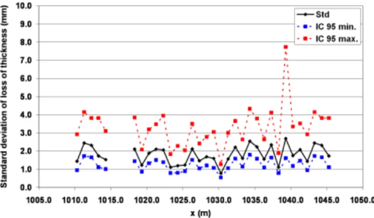
Figure 8 presents respectively the standard devia-tions of readings on out-pans for wharf HA7d.

Figure 8. Standard deviation of loss of thickness according to x – HA7d (out-pans).

The analysis of the standard deviation leads to the same conclusion as illustrated for wharf HA7d on figure 7.

Measurements don’t allow to conclude that the random field is stationary according to x. However,

the mean and the standard deviation have been com-puted from 7 measurements and in that case, the sta-tistical bias is not negligible.

3.4 Stationarity according to z

The evolution of the mean of the loss of thickness according to z for two of the three wharves, BO1 and HA7d, is presented on figures 9-11. The results concerning the third one are not presented because the amount of data is not sufficient: only 11 are available where the amount of data is 53 and 4605 for the two others. The trend appears clearly and is conform to the results published in the literature (Benaïssa 2004, Clément et al. 2008, Cetmef 2005, Memet 2000).

Figure 9. Mean of loss of thickness according to z – BO1.

For the wharf BO1, several tide levels are plotted on figures to allow comparisons with well-known profiles of corrosion:

− Mean Low Water Neaps (MLWN): the arithmetic mean of the low waters of the neap tides;

− Mean Low Water (MLW): the arithmetic mean of the low water heights observed each tidal day; − Mean Low Water Springs (MLWS): the

arithme-tic mean of the low waters occurring at the time of the spring tides observed over a specific 19-year Metonic cycle;

− Mean Lowest Astronomical Tide (LAT): The lowest level that can be expected to occur under average meteorological conditions and under any combination of astronomical conditions.

For HA7d, due to the small seawater variation in the dock (0.6 m), only two levels are indicated, i.e. High water and low water.

For wharf HA7d, measurements on in and out-pans of a U-shape sheet piling are dissociated. Mean of loss of thickness on out-pans on Figure 10.

Figure 10. Mean of loss of thickness on out-pans of sheet pil-ing accordpil-ing to z – HA7d.

Figure 11 illustrates the well-known phenomena on the U shaped piles: out-pans corrode faster than in-pans.

Figure 11. Mean of loss of thickness on in and out-pans of sheet piling according to z – HA7d.

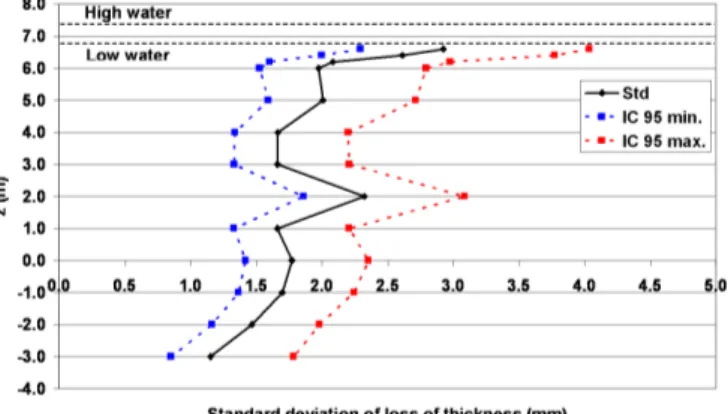
Concerning the standard deviation, Figures 12-13 il-lustrates the same trend than the mean of loss of thickness with depth.

Figure 12. Standard deviation of loss of thickness according to z – BO1.

Figure 13. Standard deviation of loss of thickness on out-pans of sheet piling according to z – HA7d.

3.5 Coefficient of variation

Mean and standard deviations having the same trend with depth, let us focus now on the evolution of the coefficient of variation with depth. Figure 14 illus-trates this evolution. This coefficient of variation is quite constant according to z. For wharf BO1, it reaches 0.47, for wharf HA7d, 0.44 for out-pans and 0.49 for in-spans of sheet piling and 0.64 for wharf HA8b where the quantity of measurements is fair and concerns only out-pans.

Figure 14. Coefficient of variation of loss of thickness accord-ing to z – BO1.

3.6 Covariance and correlation

Even if the field if not stationary, this assumption is usually made and a lot of papers starts with the plot-ting of the variogram. The covariance and the coef-ficient of correlation as functions of the distance h between measurements are plotted on figure 15 along the length x and on figure 18 along the depth z for BO1.

It is clear that no structure of correlation can be deduced according to x, in spite of the small distance h between two measurements of loss of thickness (0.15 to 0.20 m).

Figure 15. Correlation of loss of thickness according to x – BO1.

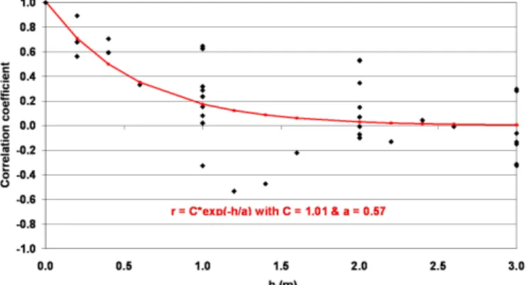
According to z however, on figure 16 for B01 and on figures 17 for HA07d, the coefficient of correla-tion seems to decrease with h.

Figure 16. Correlation of loss of thickness with h according to z – BO1.

Figure 17. Correlation of loss of thickness with h according to z – HA07d (in-pans).

Note that the correlation is significant only be-tween very close points (i.e. fair values for h) that are generally in the same area.

For HA8b, the confidence interval is too wide due to the fair quantity of data.

4 MODELLING OF THE PROCESS OF CORROSION

The aim of the modelling of corrosion process in harbours is to provide predictive models that account for the spatial dependence both in depth and in

length and the time variability in a given environ-ment E. We start from the assumption that effects of spatial dependence are decoupled along x and z. A statistical model gives the main trend with z and the trend with x comes from an analysis and a fitting.

In a given environment, these trends must account for the type of sheet piling (flat, Z or U-shaped) and eventually, the shape of the structure (wall or coffer-dam) that modifies the exposure of some sheet piles. Then the corrosion model of Melchers is extended in case of spatial trend (equation 1) (Melchers, 2003):

c(x,z,t,E,θ) = tr(x,z,t,E) + c(z,t,E,θ) (1) where c(x,z,t,E,θ) is the loss of thickness expressed as a stochastic function indexed by the abscissa along the structure x (expressed in meters), the depth

z (in meters) and time t (in years). E denotes the

cor-rosion factors and θthe hazard. Deterministic func-tion tr(x,z,t,E) denotes the centered trend of the cor-rosion field according to x.

Stochastic function c(z,t,E,θ) represents the loss of thickness at depth z, time t, in a given environment E. It is based on the model formulated by R. Melchers in equation 2:

c(z, t, E, _{θ) = b(z, t, E) fn(z, t, E) + ε( z, t, E,θ)} (2) where fn(z,t,E) denotes the deterministic trend with time at a given depth z. It is fitted on the mean value of experimental data th0(z,t,E). Depending on the type of corrosion, following forms are suggested: − Equation 3 if no presence of bio-corrosion:

(

)

j,t,E) C1 e z

(

fn = − −α (3)

− Equation 4 if presence of bio-corrosion and no possibility to identify the first stage of the model from inspections (inspection results after 10 years):

(

)

(

)

If ‘m’ structures are inspected at time t, th0(z,t,E) is the mean value obtained from the ‘m’ structures in the same environment (see equation 5):

∑

In equation 6, with an abuse of notation and consid-ering that all readings according to x are independent realizations due to hazard _θi of the same variable

(i.e. the spacing between measurements is larger than the correlation distance with x), expression of

) , E , t , z ( th0_k θ_i is suggested: ) t , z , x ( tr ) E , t , z , x ( th ) , E , t , z ( th_k0 θ_i = _{k i} − _{k i} (6)

For example, for the wharf BO1, a linear trend is convenient and it corresponds to equation 7:

⎟ ⎠ ⎞ ⎜ ⎝ ⎛ − = 2 l x ). z , t ( a ) x ( tr (7)

where ‘a’ is a deterministic function of time t and depth z describing the slope of the spatial depend-ence (mm/m) and ‘l’ the length of the structure where data are available. On figure 18, it is interest-ing to observe in the case of wharf BO1 that the val-ue of ‘a(z)’ follows the same evolution with depth as the value of the mean of corrosion loss.

Figure 18. Evolution of a(z) and mean of loss of thickness with depth – BO1.

Figure 19 gives the distribution of _{ε in the low} seawater zone and statistical parameters of ε for the three zones, i.e. tidal, low seawater and immersion zones, are given in table 4.

Figure 19. Distribution of ε in the low seawater zone – BO1. Table 4. Statistical parameters of ε for several exposure zones. ______________________________________________ Exposure zone*: ZT ZL ZI ______________________________________________ Mean 0.00 0.00 0.00 Standard deviation 1.21 1.37 1.25 Min. -2.89 -3.09 -3.27 Max. 7.78 7.74 5.66 Fractile 10 % -1.16 -1.34 -1.20 Fractile 90 % 1.67 2.00 1.79 _____________________________________________ * ZT = Tidal zone; ZL = Low seawater zone; ZI = Immersion zone.

5 CONCLUSION

Data available for the study of the steel corrosion in marine environment are measurements of residual thickness of steel by ultrasonic non destructive tech-nique at several depths and several locations along the French harbors structures.

The analysis of the stationarity of corrosion pro-cess with space is carried out from the statistical analysis of 3 wharves. The conclusion is that the sta-tionarity cannot be proved easily with the available data and that the distance of correlation of these structures is less than 0.2 m.

Moreover, characterization of the spatial variabil-ity of the metal loss of thickness of marine structures due to the corrosion is an essential stage to optimize the maintenance plans. The problem consists in inte-grating the results obtained during the various cam-paigns of inspection within the decision processes in a most realistic possible way.

The spatial variability of the corrosion cannot be objectively described in a quantitative way by de-terminist models, so a first level of steel corrosion spatio-temporal modeling in marine environment is suggested, based on the model developed by Melchers.

Now, a statistical analysis of the whole available data is necessary to confirm assumptions to model the spatio-temporal process of corrosion.

6 REFERENCES

Benaïssa, B. 2004. La corrosion des structures métalliques en mer : types et zones de dégradations, VIIIèmes Journées Na-tional Génie Civil – Génie Côtier, Compiègne, 7-9 sep-tembre 2004.

Cetmef. 1995. Surveillance, auscultation et entretien des ou-vrages maritimes, Fascicule 3 : Quais sur pieux, Notice STC PM 95.01.

Clément, A., Boéro, J., Schoefs, F., Memet, J.B. 2008. Over-view of corrosion impact for marine structures : analysis of French structures in several harbours, 1st International Con-ference MEDACHS (Construction Heritage in Coastal and Marine Environments. Damage, Diagnostics, Maintenance and Rehabilitation) – Interreg IIIB Atlantic Space – Project n°197, Theme 3: Service life modelling and reliability, Lis-boa, Portugal, 28-30 January 2008.

Melchers, R.E. 2003. A new model for marine immersion cor-rosion in structural reliability, Applications of Statistics and

Probability in Civil Engineering, Ed: A Der Kiureghian, S

Madanat and JM Pestana, Millpress, Rotterdam, 599-604. Memet, J.B. 2000. La corrosion marine des structures

métal-liques portuaires : étude des mécanismes d’amorçage et de croissance des produits de corrosion. Thèse de doctorat, Université de La Rochelle. 164 p.