The Reciprocity Gap Functional for Identifying Defects and Cracks

HAL Id: hal-00112504

https://hal.archives-ouvertes.fr/hal-00112504

Submitted on 13 Dec 2019

HAL is a multi-disciplinary open access

archive for the deposit and dissemination of sci-entific research documents, whether they are pub-lished or not. The documents may come from teaching and research institutions in France or abroad, or from public or private research centers.

L’archive ouverte pluridisciplinaire HAL, est destinée au dépôt et à la diffusion de documents scientifiques de niveau recherche, publiés ou non, émanant des établissements d’enseignement et de recherche français ou étrangers, des laboratoires publics ou privés.

The Reciprocity Gap Functional for Identifying Defects

and Cracks

Huy Duong Bui, Andrei Constantinescu, Hubert Maigre

To cite this version:

Huy Duong Bui, Andrei Constantinescu, Hubert Maigre. The Reciprocity Gap Functional for Identify-ing Defects and Cracks. Zenon Mróz; Georgios Stavroulakis. Parameter Identification of materials and structures, 469, Springer-Verlag, pp.17-54, 2005, CISM International Centre for Mechanical Sciences, 9783211381342. �10.1007/3-211-38134-1_2�. �hal-00112504�

The Reciprocity Gap Functional for Identifying

Defects and Cracks

H.D. Bui, A. Constantinescu and H. Maigre Laboratoire de Mecanique des Solides, CNRS,

Ecole Polytechnique, Palaiseau, France

Abstract. The recovery of defects and cracks in solids using overdetermined boundary data, both the Dirichlet and the Neumann types, is considered in this paper. A review of the method for solving these inverse problems is given, focusing particularly on linearized inverse problems. It is shown how the reciprocity gap functional can solve nonlinear inverse problems involving identification of cracks and distributed defects in bounded solids. Exact solutions for planar cracks in 3D solids are given for static elasticity, heat diffusion and transient acoustics.

1. Introduction and Scope

There are many classes of inverse problems for detection of defects in solids: recovery of distributed coefficients, densities, identification of cavities and cracks.

The recovery of coefficients or densities in a domain from line integrals, known as "Ray Tomography", with X-rays or Gamma-rays, single or double photon emission ... is possible owing, on the one hand, to highly sophisticated data acquisition systems such as Scanners, Photonic Collimators and, on the other hand, to mathematical techniques like the Radon transform and its exact inverse, with or without absorption. The case of Gamma ray tomography, taking account of the Compton electron diffusion, has been investigated recently by Nguyen and Truong (2002) and Nguyen et a! (2002) who gave the exact inverse of the so­ called "Conical Radon Transform". For optical absorption and scattering tomography, the

mathematical models are given by the Boltzmann transport equation and the diffusion equation. For a review of the topic, see Arridge ( 1999).

Applications of acoustics in geophysics and non destructive testing of materials are based on mechanical set-ups like the transducers which collect data on their boundary. Mathematically one deals here with inverse scattering theories which are based on some approximations: incident plane waves, Born's approximation, Kirchhoffs approximation (see Bui, 1993, 1994). Analytical solutions exist only for some specific problems. For example, in "Acoustics tomography", under the above approximations, an exact solution to the inverse scattering of a rigid inclusion has been given by Bojarski (198 1 ). The classical "Elastic Wave Tomography" using the Kirchhoff approximation, the far-field analysis and the assumption of smallness of the defects, leads to the so-called POFFIS method (Physical Optics Far Field Inverse Scattering). Most works applied to Geophysics are generally based on numerical methods such as Finite Elements Method, Boundary Integral Equations, Optimal Control theory ( Lions, 197 1 ).

Recently a large amount of work has been devoted to "Generalized Tomography" applied to different physical phenomena ranging from elliptic to parabolic and hyperbolic equations. Such works are yet at the stage of primary developments of methods for computational and for pure and applied mathematical purposes. Despite the existence of new devices such as the Infra-Red camera already used for investigation of delaminations in composites structures or functional observations in Biology, its industrial applications are not well developped. One explanation is the lack of exact solutions to thermal inverse problems which can be used as a benchmark for computational solutions and, above all, the difficulties encountered in numerical methods for ill-posed inverse problems.

The aim of this paper is to review some recent works done in the applied mathematics for identifYing defects in solids. It focuses mainly on the following topics:

a. Derivation of the "Observation Equation" using the notion of"Defect Indicators". b. General considerations on non-linear and linearized inverse problems.

c. Linear inverse problems settings; Ill-posedness; Regularizations methods; Mathematical aspects; The Cauchy Problem.

d. Exact solutions of the inverse problems for identifying a planar crack in the 3D case, for elliptic, parabolic and hyperbolic equations, from overdetermined boundary data. 2. Defects and cracks indicators

The boundary data for recovering the defects provides qualitative and quantitative informations about the unknowns by means of defect indicators. If there exists a relationship between the boundary data and the parameters which characterizes the unknown defects, this relationship can be used as a defect indicator. Generally the indicator is a boundary integral which vanishes in the case of absence of defect or relates to the strength of the singularities inside the body, the location of point forces, or the crack geometry, etc.

The method for obtaining indicators are based on conservation laws which transfer the information about the mechanical field inside the body to the exterior boundary S where boundary data can be obtained, without solving any boundary value problem. Let us consider

some types of indicators in the following examples. Consider a first class of indicator defined by a conservation law of the form -div(A)=B in n, with B a source term.

The defect indicator is given by the boundary integral

I =-

f s

A.n dS ( 1 )

over the exterior surface S of the body. The integral (I) vanishes (or not) if B=O (or Bf':O), indicating the abscence (or presence) of the source. As an example, consider the stress field cr(x) in a 3D solid,

- divcr(x) = fo(x-a) in Q (2)

with the point force fO(x-a). The integral ( 1 ) is equal to the total force f.

Consider another class of indicator more general than ( 1 ), in the case of linear elasticity under small strain. Denote by cr[u](x) the stress field corresponding to the displacement field u(x) in the solid due to the point force tO(x-a). Introduce an auxiliary field cr[ v ](x) associated to the displacement field v(x), without body force. We get

- div{cr[u].v - cr[v].u} = v. f o(x-a) in n (3)

The indicator derived from (3) is the linear form v �I(v)

I(v) = -

fs

{n.cr[u].v- n.cr[v].u}dS (4)

which contains the information on both the force f and the point a.

This indicator is twice the bilinear symplectic form corresponding to the energy release rate in linear Fracture Mechanics.

Exercices. Take v=(vj), vj=Oij and verify that I(vj)= fi. Take v=(vj), vrxkoij and verify that I(vj)= akfi. + 2.1. Crack indicator

Let us introduce another class of indicators more suitable for crack detection. We assume that the stress field cr[ u ](x) corresponds to the stress field of the previous 3D elastic solid with an unique internal crack �. with some boundary conditions on S and without body force. We assume that v( x) corresponds to the auxiliary (or adjoint) field of the uncracked solid, with the same elastic constants and some different boundary conditions. The indicator given by (4) is called here the Reciprocity gap R(v)

The reason of the word "gap" in the name comes from the fact that in an uncracked body, the Betti reciprocity relation yields R(v)=O, for any v satisfying the elasticity equation. Hence a non vanishing value of R(v) indicates the presence of a crack. More precisely by introducing the displacement jump defined as [[u]]=u+ -u-one gets

R(v) =

JL:

n. cr[v].[[u]]dS (6)

where n = n-= -n+. From (5) and (6) one obtains the "observation equation"

JL:

n. cr[v].[[u]]dS=

fs

{n. cr[v].u- n. cr[u].v}dS (7)

Equation (7) has been derived in many works as a tool for crack identification. It can be generalized to transient problems in elasticity, acoustics, and also to heat diffusion problems (See Section 7.2). The use of (7) for crack identification using an overdetermined boundary data pair (u, T:=n. cr[u]) will be discussed in Section 7. Let us remark that Equation (7) alone is not sufficient for identifying the crack I:. We shall discuss further two important questions : the number of data pairs (u, T) and the nature of adjoint fields which are necessary and sufficient for a complete identification. The identifiability question is important because it is related to uniqueness of the solution of the inverse problem for exact data pair. In contrast with the identifiability problem, practical solutions to crack or defect inverse problems are based on numerical computations which generally make use of noise-contamined data pairs. In this case, the key issues are the continuity of approximate solutions with respect to data variation and an error estimate with respect to the exact solution. These questions will be examined for linear inverse problems which are simpler than nonlinear inverse problems.

2.2. Distributed Defect Indicator

The following example is given by Calderon ( 1980) for transient as well as for static heat diffusion equation. Let us restrict to the static case. Distributed defects in solids are due for example to the presence of microscopic voids and micro-cracks which change macroscopically the thermal diffusion coefficient, from the known constant value k0 to k(x)=ko+c(x).

Without lost of generality, we consider normalized constant so that k0=1 and assume that c(x)=O on oQ. In the macroscopic scale, c(x) can be considered as the damage field.

The inverse problem consists of finding c(x) from measurements of surface temperature 8 and temperature gradient B n8.

The equations are the following ones. -Actual field 8 (damaged solid) :

- div{ ( l +c)grad 8} = 0 (in Q) (8)

-Adjoint field \jJ (undamaged solid):

- divgrad \jJ = 0 (in n) (10)

(on on) (11 )

The observation equation i s given by :

(12) The explicit dependence of8[c] on c in Equation ( 1 2) and the solution of (8) and (9) under the compatibility condition DJanfdS=O clearly show that the observation equation is nonlinear with respect to c.

The observation equation (12) alone does not allow the determination of the scalar field c(x) since its right hand side is a scalar constant denoted by d, for a given surface data pair (8,on8) and for a given adjoint field \j.l(x). It is necessary to establish an one-to-one mapping between c(x) and a larger family of data d(i;;) depending on some family of boundary data or of adjoint fields indexed by some N-dimensional parameter i;;.

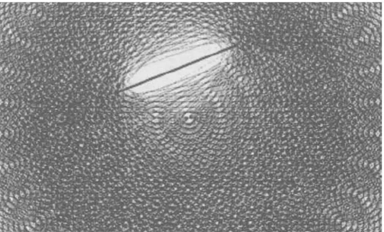
To illustrate the necessary condition, suppose for example that c(x) is a constant c inside a 2D ellipsoidal inclusion, and is equal to zero outside the inclusion, Figure I. To determine the constant c and the ellipsoidal geometry, e.g. 6 unknown parameters (the constant c, 2 coordinates of the center, the orientation of the main axis, the semi axes a and b), many procedures can be used. One can consider a single data pair (8,8n8) measured on an and six adjoint fields, or two data pairs (81 ,8n81), (82,8n82) and three adjoint fields etc. These conditions are necessary but not sufficient for solving the nonlinear inverse problem.

Calderon ( 1 980) proposed a linearization of (12) in order to obtain a simpler inverse problem, which can be solved exactly for 3D defects. His basic idea is the consideration of a 3-dimensional family of boundary data fz(x) and g2(x), with z being a 3D vector.

The linearized inverse problem is based on the first order approximation of ( 1 2), considering c as a small perturbation. The linearized observation equation for the first order solution c� is deduced from ( 1 2) by leaving the right hand side of( 1 2) unchanged and changing only the left hand side as

fo

c�grad<j>. grad\jf dV =

fan

(\jf f- 8 g)dS

where <J> is the solution of the boundary value problem on the solid without defect : - div {grad<J>} = 0 (in Q)

on<J>(x) = f(x) (on on)

( 13)

(14) ( 1 5) By taking a family of boundary data fz(x) and g2(x), ZER3, the right hand side of ( 1 3) becomes a scalar field d(z) and equation ( 1 3) becomes a Fredholm integral equation of the first kind for c�(x) with kernel K(x, z)=gradx<J>(x; z).gradx\jf(x; z). As expected, the linear inverse problem for c� is ill-posed because it is governed by a Fredholm integral equation of the first kind mapping the x-space onto the z-space.

An attempt to solve the nonlinear equation has been given in (Isaacson and Isaacson, 1989) for determining c(x) within a circular inclusion (a priori knowledge on the shape). A surprising result was found for the supporting function supp[ c] which takes the values 0 or I, depending on whether c(x)=O or c(x)#). It is found that the support functions of c(x) for nonlinear theory and c�(x) for linearized theory are practically the same. The result is very interesting for applications because it justifies the use of the linearized theory, even when c(x) is not small.

A recent study (Bui and Constantinescu, 2000) on the detection of damage in elasticity using integral equation techniques gives a similar result. Far from the inclusion and the boundary, where c(x) is assumed to be zero, the difference in the stress components between nonlinear and linearized theories is found to be negligible.

In the next section, we reconsider the comparison between nonlinear and linerarized theories for the stationary heat equation.

3. Nonlinear and Linear Theories

Consider the inverse problem for determining an internal perturbation c(x), using the boundary data 8(x)=h(x) and on8(x)=f(x). Instead of comparing c(x) with c�(x), we compare the nonlinear solution 8NL(x) with the thermal field 8L(x) associated with the linear theory. We assume

i) that the perturbation is continuous and admits a series expansion in the form c=�::cl+�::2cz+ . . . with small �:: and,

ii) that the supports Zi of the functions ci(x) are compact and that ci(x)=O on oZi and outside Zi. The support Z of c(x) is given by the union of the Zi's. A well-known example of such compact support functions is given by the test functions in finite element methods.

The field 8(x) satisfies the Dirichlet boundary value problem: - div{(l+c)grad8} = 0 (in Q)

8(x) = h(x) (on 8Q)

( 1 6) ( 1 7) and admits the series expansion 8(x)=8o+!>81(x)+!>282(x)+ .. . The nonlinear thermal field 8NL(x)=8(x) admits the integral representation (88/8n = f(y))

8(x) =

fan

{G(x,y)f(y)- h(y)an

p

(x,y) }dSy +

fz

G(x,y)div{c(y)grad8(y)}dVy ( 1 8) where G(x,y) is the Green's function. We call 80(x) the zero-order solution satisfying the equations:

- div{grad 8o} = 0 8o(x) = h(x)

(in Q) (on 8Q) The zero order term 8o(x) admits the integral representation

In what follows, the sum of the first two terms will be refered to as the linear solution ( 1 9) (20)

(2 1 ) B y substituting the series expansions o f c(x) and 8(x) in ( 1 6) and ( 1 7) and considering the term 0(!>), we obtain the governing equations for e,(x)

- div{grad 8 J } = div{c1(x)grad8o(x)} (in Q) (22)

(on 8Q) (23)

The field e,(x) admits the integral representation

Using the boundary condition c 1(y)=O on az" it can be shown that the difference � between the nonlinear solution and the first order solution is given by

� =8NL(x) - 8L(x)

=fan

G(x,y) {8ny8- 8ny8o - !>8ny8J }dSy

Both terms of the right hand side of (25) are of order 0(�::2). By differentiating (25), we obtain the difference between their gradients r =gradxl1

r(x) =

fao

gradxG(x,y) {anye - anyeo -�::anyel } dSy

- (fp) �::2

f

z1 gradxgradyG(x,y)cJ(y)grady91 (y)dVy x�(ZJuan) (26) where (fp) stands for the Hadamard finite part sense. A close inspection of (26) shows that the difference between the thermal gradient is significant only inside or near Z::::>ZJ because of the following reasons :

1 . the kernel of the first term behaves as lgradxGI"'='Ix-yl-2, with lx-yl=distance(x,aO). Therefore the first integral term is significant only in the vicinity of an, due to the difference in normal derivatives an 9 -an (9o +�::91)"'='0(�::2). Note that in the derivation of the approximate solution, c-(x), it is a

ls

ume

l

that the same normal derivative holds for SL(x) and 9(x) so that

{an e -an (9o+&9J)}<"='0.

2.

th

l

second term, understood in the Hadamard finite-part sense, decreases as lgradxgradyGI"'='Ix-yl-3, as the distance r =distance(x, Z1 ) increases.

The difference 11 between nonlinear and linear thermal fields decreases as the distance to Z1 increases, and the decrease of r is much more rapid.

These analyses show that far away from z1 we find that the thermal fields SNL(x), 9L(x) and their respective gradients gradx9NL(x), gradx9L(x), are quite similar. In other words, the perturbation of the thermal coefficient c(x) is not significant outside Zl' while by assumption, the perturbation �::c1 (x) vanishes outside Zl ' consequently vanishes too outside Z (which contains the subset Z1 ).

This discussion indirectly shows that the property observed in (Isaacson and Isaacson, 1 989) about the support of the nonlinear solution c(x) for circular inclusion and that of the linearized theory c-(x), in the Calderon sense, Equation ( 1 3), seems to be likely for an arbitrary geometry of the inclusion.

Remark 1. The example of the thermal inverse problem shows that a relationship between the unknown coefficient k(x) and the boundary data pair d={Sd, aned} can be written formally as A(k)=d, where A is a nonlinear integral operator, the kernel of which is defined implicitly by equations (8) and (9). A simpler approximate observation equation is derived in discretized form, if we set k={kJ, k2, k3, ... kn} . By means of the Finite Element Method, one solves (8) and (9) using the Neumann boundary condition ane=f (or an9d) and calculates the boundary temperature ecal(kJ, k2, k3, ... kn). The inverse problem is defined as the optimization of an objective function.

Generally, the least square method is used to minimize the "error" between predicted and measured temperatures

k= arg Mink

I

ecal(kJ, k2, k3, ... kn) - ect

1

2

The difficulty of such numerical approach lies on the evaluation of the gradient of the error functional with respect to ki which requires a great number of solutions of the equations (8) and

(9) for different increments 8ki. It can be overcame by using adjoint equations (See, e.g., Constantinescu, 1 995 ).

Alternatively, instead of using the Neumann bounadry condition, one can solve the thermal equation with the Dirichlet boundary condition 8=8d and then calculate the optimal flux 3n8cal(k!, kz, k3, ... kn) which approaches the datum 3n8d

A symmetrical method consists of minimizing the "constitutive law error functional" (see Kohn and Vogelius, 1 984 and Constantinescu, 1 994, 1 995).

F(q, 8, k) = ( 1 /2)

fn

(k112grad8 + q k-112)2dV

where the field 8 satisfies the Dirichlet boundary condition 8=8d while q satisfies the equilibrium equation div(q)=O and the Neumann boundary condition q�f (k=l on the boundary). The constitutive law

q + kgrad8 = 0

is solution of the minimization of the "polyconvex" functional F, convex with respect to each variable separately, but not convex with respect to all together.

Remark 2. The nonlinear equation A(u)=y, uEX, yEY is generally solved by methods of linearization. It is assumed that the Frechet derivative A'(u) exists. The least square method leads to the minimization problem Minu \\A(u)-yjj2, with the norm jj.jj in the Y-space. The solution is obtained formally by the multistage quadratic programming which, starting from a guess value (or a priori knowledge) uO, calculates the updated solution uk+ 1 =uk+sk with

sk =Arg (Mins \\A(uk) + A'(uk)s- yjj2), s EX.

Each stage ofthe calculation of sk corresponds to a linear inverse problem A'(uk)s=d, with d=y-A(uk).

4. Linear Inverse Problems Settings in Hilbert Spaces

Let X be the set of unknown model parameters and Y be the set of observable or accessible data used for recovering unknown parameters. By model parameters we include unknown mechanical fields, unknown geometry, material constants etc.

Consider two Hilbert spaces (X, (.,.)x , jj.jj) and (Y, (.,.)y, j. \) with inner products (.,.)x, (.,.)y, and respective associated norms jj.jj, j. j. We consider a continuous linear mapping A from X to Y, which arises in many inverse problems or in the linearisation procedure of nonlinear problems. We assume that the map A and its adjoint A* are bounded. For given

datum dEY, one considers the problem of finding the solution of the so-called «observation equation » :

Au=d , u E X, d Ey (27)

One important difference with usual direct problems is that inverse problems are generally ill-posed. This means that A is not always invertible, or solutions do not always exist, and in the case of existence of solutions, these solutions do not depend continuously on the data. The sensitivity of the solution to errors in data is the very common feature of ill-posed problems.

It is necessary to introduce a « regularization » process in order to obtain a well-posed problem, which is required to be « close » to the initial one. These two objectives - good mathematical property in the regularization process and physically acceptable model - are often so contradictory that, according to P. Sabatier ( 1987), their satisfaction may be rather a matter of « Art » than « Sciences ».

The equation (27) can be writen in the variational form

(Au, Av)y = (d, Av)y , UEX , dEY , VvEX (28)

does not have an unique solution, because the bilinear form (Au, Av)y is not assumed coercive. Regularization techniques, introduced in (Tikhonov and Arsenine, 1 976, 1 986), consist in the construction of « solutions » stable with respect to the variation of the datum d, by « changing » slightly the map A, or by introducing coercive variational equations.

4.1 Coercive Variational Equation

We introduce an additional term (a >0) in the variational equation (28)

(Au, Av)y +a(u, v)x = (d, Av)y , UEX , VvEX (29)

The added term ensures the coercivity of the bilinear form which can be rewritten as

((A*A+al)u, v)x = (A*d, v)x , UEX , VvEX (30)

where (A* A +al) is invertible. The solution of the modified equation (29) is

u(a) = (A* A+ar)-1 A *d (3 1 )

A large constant a leads to unphysical solution, while a too small value of the constant a yields unstable numerical solutions. There exists an optimal choice of the regularizing parameter, proposed by Kitagawa ( 1 987). But this optimal choice is not essential for the following discussions. It is important to observe that if the solution u of (28) exists, the solution is unique only when A is strictly positive A>O and that the solution u(a) in (3 1 ) with the same datum d tends towards the exact solution u in X, Jlu(a)-uJI�O, as a�O. However, in

most inverse problems for identifying defects and cracks, the condition A>O is not always satisfied.

Remark. It is worth mentionning a geometrical interpretation of the Tikhonov regularization procedure. Suppose that there is an a priori knowledge about the solution of (27) given by the constraint llu-u011<� with known u0 and �>0. An approximate solution of (27), with an a posteriori residual error c;>O, is given by any u belonging to the intersection C of two convexes IAu-dl<c: and llu-u011<�. Either the intersection C is void (no solution to the

inverse problem exists) or not void (there is an infinite number of approximate solutions). In the latter case, one possible solution can be chosen as follows.

Let us remark that the intersection C is bounded by two ellipsoids, C2 =>C::::>CJ, from below by the set C1 ofu such that IAu-dl2/c:2 +llu-u0il2/�2�1 and from above by the set C2 ofu such that 1Au-dl2/c:2 +llu-u0ll2/�2�2.

A solution (not unique) satisfying the constraints IAu-di<E and llu-u011<� is given by the common centre of cl and c2 or by the solution of the minimisation problem

(32) with a=c;2j�2 which can be interpreted as the Lagrangian multiplier. The solution of the

minimization problem (32) is unique and given by

u(a) = u0 + (A*A+al)-1 A*(d-Au0) (33)

4.2 Continuity Property

Mathematically, the regularized solution u(a) depends continuously on the datum d. This is the consequence of the Lax-Milgram theorem, based on two properties :

1 . A*A+al is bounded, 2. A* A+al is coercive.

The linear operator A* A : X �x is self-adjoint and positive, but not strictly positive. For the continuity property and the convergence property as a�O, see the following Exercices.

Exercice. Proof:

Exercice.

Prove the inequality: II u(a)(d) - u(a)(d')ll � a-ljiAII-Id-d'l, for any d, d'. Consider two data d, d' and the corresponding solutions u, u' of (29). For convenience we write simply u=u(a)(d) and u'=u(a)(d').

By substracting the corresponding bilinear forms one gets: (A(u-u'), Av)y + a(u-u', v)X = (d-d', Av)y VvEX ::::> (A*A(u-u'), v)x + a(u-u', v)x = (d-d', Av)y VvEX

Take : v = u-u' , one gets

IIA*AII-IIu-u'll2 + allu-u'll2 � IIAII-Id-d'l.llu-u'll => => allu-u'll2 � IIAII ld-d'l-llu-u'll => allu-u'll � IIAII-Id-d'l •

Proof : (Au, Av)y = (d, Av)y VvEX

(Au( a), Av)y + a(u(a), v)x = (d, Av)y VvEX (A(u(a)-u), Av)y + a(u(a), v)x =0 VvEX Take: v= u(a)-u, one gets

I lA (u(a)-u)ll2 + a(u(a),u(a)-u)x =0 :::::;, a(u(a),u(a)-u)x :o; 0

::::::> llu(a)ll2 :o; ( u(a), u)x :o; II( u(a)ll.llull ::::::> llu(a)ll:o;llull (34) Since the sequence llu(a)ll is bounded, there exists a subsequence converging weakly towards u, (u(a)-u, v)x�O, Vv.

Take v=u we obtain (u(a)-u, u)x�O. Consider now:

llu(a)-u 112 = (u(a),u(a)-u)x - (u, u(a)-u)x

Using the inequality (34), one obtains the inequality llu(a)-ull2 :o;-(u, u(a)-u)x

Therefore llu(a)-ull2 :o; -(u, u(a)-u)x �0 as a�O, hence llu(a)-uii2 �0. The sequence u(a) converges strongly towards u+

4.3 Error Estimate

One important point in mathematical works is to derive the error estimate with respect to the (yet unknown) exact solution uex. There are some results reported in the literature for Inverse Problem in Hilbert spaces settings. The main point is to make a comparison between the regularized solution u(a)(d) and the exact one uex, even if the exact solution uex is not yet known.

What is the meaning of« exact » solution ?

Let us introduce some terminologies. A pair { uex, dex } is called exact or compatible if it satisfies the observation equation

The given data dex may satisfy some compatibility condition for the existence of an unique exact solution uex in X. However it is not always possible to write explicitly the compatibility condition on dex, even if precise informations on the physical nature of the problem are known. There is of course some exception (As an example, we keep in mind the condition on the Neumann boundary data for the Laplace equation fanudS=O).

In practice, to obtain such a pair, one can take for example some uex and define dex as the direct image Auex. Such a construction of the exact pair { uex, dex } is based on the solution of direct problems which gives indeed a compatible pair with respect to the inverse problem in consideration.

The knowledge of an exact pair, given by solutions of direct problems, is useful for checking the algorithm of approximate numerical solutions. One considers a model with known geometry and materials constants and known boundary conditions data for calculating {uex, dex} . Then one makes use of the numerical data dex for recovering the approximate numerical solution u(a) of the inverse problem.

Af!other constructive solution from given data dex, consists of establishing explicit formulae giving the solution uex. Exact solutions given in Section 7 fall in this category of constructive solutions.

The main result in error estimate is stated in the following theorem.

Suppose that there exists d 1 such that uex=A *d 1. Then, the error JJu(a)_uexll is given by (35) The proof is given in the next Exercice.

The estimate (35) depends on both the regularisation parameter a which introduces some error on the modelling and the error on the datum ld-dexl in comparison with the compatible one. One gets the best possible error estimate by taking the regularization parameter proportional to the datum error a=kE

Exercice. Proof:

Suppose that there exists d 1 such that uex=A *d 1 , prove the estimate (35). The exact pair (uex, dex) satisfies the variational equation

(Auex, Av)y = (dex, Av)y VvEX, (36)

The approximate solution (u(a), d) satisfies the equation (Au(a), Av)y + a(u(a), v)x = (d, Av)y VvEX

which can be written as :

(Au( a), Av)y + a(u(a)_ uex, v)x + a(uex, v)x = (d, Av)y VvEX (37) Combining (36) and (37) we get:

(A(u(a)_ uex), Av)y + a(u(a)_ uex, v)x + a(uex, v)x = (d-dex, Av)y VvEX Take v= u(a)_ uex, one obtains

I A(u(a)_ uex)l2 + aJJu(a)_uexll2 = (d- dex, A(u(a)_ uex))y

- a(uex, u(a)_ uex)x (38)

The last term can be written as

a(uex, u(a)_ uex)x = a(A*d1, u(a)_ uex)x = a(d1 , A(u(a)_ uex))y The left hand side of (38) is bounded by

I A(u(a)_ uex)l2 + aJJu(a)_uex/12 � ld-dexl. IA(u(a)_ uex)l + ald11 .1A(u(a)_ uex)l � IA(u(a)_ uex)l. (ld-dexl + ald11) � IA(u(a)_ uex)l2 + (1/4) (ld-dexl + ald11?

Finally, by using ld-dexl< f: and a=kE, one obtains the inequality (35) aJJu(a)_uexJjZ � (1/4) (ld-dexl + ald1 1)2

=> llu(a)_uexll � (1/2) a-112 (ld-dexl + ald11) +

5. Geometry Bound Methods for Static Problems

It is often of interest to determine, not exactly the geometry of defects and cracks, but only their approximate location in the solid. Geometry bound methods consist of determining spatial subdomains which do not contain internal defects and cracks. The initial inverse problem of determining defects or cracks in Q, using the boundary data pairs {u, 8nu} for Laplace's

equation, or {u, T[u]} for elasticity, is replaced by a set of inverse problems for smaller and smaller domains Q', with new data pairs to be determined for oQ'. The condition to be checked is that the spatial domain z between s (exterior boundary of oQ) and s' (exterior boundary of oQ') must be free of defects.

Mathematically, for elliptic equations such as the Laplace equation, the transfer of the boundary data pair {u, onu} from S to S' is called analytical continuation or Cauchy's problem. It is not the purpose of the present paper to make an extensive review of Cauchy's problems for elliptic equations, in particular for the Laplace equation. There are some important mathematical works devoted to such problems, Laurentiev ( 1 967), Lattes and Lions ( 1967). We shall mention only some of them, particularly a new approach suitable for applications in engineering problems, which makes use of explicit computations using transfer matrix operators for solving inverse problems. Different methods can be used for solving Cauchy Problems.

1 . Trial and error of the boundary S'. For the trial S', solve the Cauchy problem in Z, then use of an analyticity criterion to check the continuation inside Z. In the example of distributed damage, c(x) must be zero inside Z. Equivalently, the defect indicator must be zero for the boundary oZ= {S, -S'} . Two methods allow the determination of the solutions inside Z, the Quasi-reversibility Method introduced in (Lattes and Lions, 1 967) and the Moment Method (Dang-Dinh et a!, 2002).

2. Step-by-step continuation of the field from S to the inside until the appearance of singularities (cracks, discontinuity of gradients etc). The change from S to S' is infinitesimal and the solution is obtained by means of the Transfer Matrix Operator (Bui, 1 993, 1 994). The second method is suitable for numerical solutions to static and transient problems.

5.1 Ill-posed ness of the Cauchy Problem

Let us illustrate some methods for 2D geometries. Consider an inverse problem for a square with the superabundant data u=l and g:=onu=-1 given on x2=0, while u=l + x2 on the lateral boundaries x1=0 and x1= 1 . Find u and the normal derivative o2u on the side xz=l . The analytic solution is u(x1 ,xz)=l +xz. This classical example given by Hadamard ( 1952) illustrates the ill­ posedness of the inverse problem.

Let us assume that the first boundary value u=l on x2=0 is perturbed by a small noise of the sin-form

u(x1 , 0) = 1 + Esin(2krcx1)

with small wave length Ilk, and small amplitude E. At a first sight, the additional term is small in the sense that both 1/k and E are small. But the small perturbation yields a large change of the expected normal gradient ozu on xz=l given by

ozu(x�o 1 ) = 1 + 2krcE sin(2krcx1 )sinh(2krc) (39) This gradient blows up exponentially as k�oo. This phenomenon illustrates the sensitivity of the solution to data errors. In the case of identification of a crack from Cauchy's data,

without any constraint on the geometry of the crack, one can expect an oscillatory solution under small perturbation of data (star-like geometry, sea urchin geometry etc.). To limit the oscillatory solution on the defect geometry, one considers the constraints such as bounded length, smooth curve, etc to be imposed as a penalty on the error functional in optimisation methods. The determination of cracks by solving Cauchy's problems is considered in the paper (Alessandrini et al, 1 999), where the best possible stability estimates are given. For the determination of an unknown smooth crack r in 2D, with Dirichlet condition, one assumes that the length of the crack is bounded. This is an a priori knowledge which is a constraint for regularizing the Cauchy problem. A stability result of the type dH(r,r')�A(logllog�::l)-112, with �:: the error in Cauchy's data, is given in (Alessandrini, 1993). The «distance » between two solutions r, r' is the Hausdorff distance between two curves

dH(r, r') = max{ supxEr dist(x, r'), SUPx'Er' dist(x',r)} .

The regularisation procedures for solving the Cauchy problems are specific for each case. In next sections, we make a review of some methods for static inverse problems.

5.2 The QR Method

The Quasi-Reversibility method (Lattes and Lions, 1 967) applies to a variety of problems, governed by elliptic, parabolic equations etc.

Consider the Cauchy problem for the Laplace equation. The QR method relies upon the use of a higher-order (4th order) partial differential equation defined herafter, depending on a small parameter �::, whose solution u( �::) is identical to the harmonic function u in the domain Q, except in a layer of thickness 2�::.

Let us consider a square domain Q :={xi O<xr<I, O<x2< l } . Consider Q(2c):={xl O<x2< l -2�::}, C(c):={xl l-�::<x2< 1 } . The domains Q(2c) and Q share a common boundary denoted by r, where the data are given u=ud and g:=anu=gd.

The Cauchy problem is equivalent to the problem of finding u(!::) solution of the problem : L'l(M(c)2 L'lu(c)) = 0 in Q(2�::)

u(c) = ud and g(c) := anu(c) = gd on r where M(c)(x) is a C2 continuous and positive function defined in Q Dby :

M(c)(xb x2) = I xEQ(2�::) M(c)(xJ, x2) = 0 XE c(�::)

(41 )

and M(c)(xbx2)=0 continuous for l -2�::<x2<I-�::. Since M(c)(x\.1)=0, no other conditions are required for u(c) and v on the boundary x2=I.

The uniqueness of the solution u(E) as well as the L2-convergence u(E)�u are proved in (Lattes and Lions, 1 967). Finally, the ill-posed Cauchy Problem is replaced by a well-posed one using a higher-order equation.

No explicit regularization procedures are needed because the functions space H2(Q) considered in the variational formulation of the fourth order equation ( 40) are implicitly more regular than the space Hl (Q) considered in the original variational of the second order equation. The variational problem consists of finding u(E)EX, X being the set of function in H2(Q) satisfying (41) such that :

(M(E)�u(E)), M(E)�v) = 0, for any v EX(O)

and X(O) being the set of test functions v E H2(Q) satisfying v=O and anv=O on r. A better result can be obtained by using the penalty form of the variational equation

(M(E)�u(E)), M(E)�v)/g2 + (r(E)gradu(E), r(E)grad v) = 0 for any v EX(O) .

In the above equations the duality (.,.) means the integration over Q(E) of the product of dual terms. The function r(E) is defined by any continuous function such that r(E)=1 for x2<1-E, and r(E)= (1- x2)/E for 1 -E<x2< 1 . The L2-convergence u(E) �u, to the solution u of the Cauchy problem, is given in Lattes and Lions ( 1 967).

5.3 The Moment Method

There is an important class of Cauchy problems for the Laplace equation with discrete superabundant data pairs given on the boundary. Consider a 2D Cauchy problem of determining the flux g=80u on a known interior boundary Sint from data partially known on the exterior boundary Sext· The flux g is known on the exterior boundary Sext and the potential u is known on a bounded sequence of points (x 1 ,yJ), (x2,Y2), .. , (x0,y0) on a line segment Lo of the exterior boundary. The boundary an consists of the exterior boundary Sext and the interior boundary Sint· Measurements performed in a sequence of points may be the best possible way for gathering experimental data.

This problem is solved by the moment method (Dang-Dinh Ang et al, 2002). The uniqueness of the solution of the inverse problem is proved in the latter reference which makes use of the boundary integral representation ofharmonic functions with the Neumann type

u(x, y) = a+

f

sext N(x,y;p,q)g{p,q)dS(p,q) +

f

sint N(x,y;p,q)g(p,q)dS(p,q)

where a is a constant and N(x,y;p,q) the Neumann function for Q. Let Lo be defined by y=k. Substituting the values (x0,y0=k), n=l ,2,3 ... for the sequences of points in Lo in (41) and putting the unknowns a and z(t)=g(i;(t),f](t)), with the parameter tE [0, 1] describing the interior boundary Sint in the l.h.s. and known quantities d in the r.h.s., one gets the observation equation settings in Hilbert spaces X, Y with the linear map A :

A(a,z) = d(a,z) EX, (42) - X is the Hilbert space of unknowns u:=(a, z), X={(a, z) : aER, z(t)EHI (O,l ), z(O)=z(l )}, where z(t)=g(p(t), q(t)), and (p(t), q(t)), tE [0, l ] describes the interior boundary Sint· The norm in X is II( a, z)llx= (a2 + llzll2) 112.

- Y is the data space of sequence numbers

d := {dn}n21 E Y

dn= (1/n) (u(xu,k) -

fsext

N(xu.k;p,q)g(p,q)dS(p,q) ), ld I = (Ln21ldn I:� 2) 112 < oo

- A(a, z) is the sequence of numbers

A( a, z) :=

{

(1/n) (a +

J

[O,I] N(xn,k;p(t),q(t))(lp'(t)12+1q'(t)121)112z(t)dt)} n21 E Y Equation (42) has been put in the standard form (27) or in the variational form (28) for which Tikhonov's regularisation procedure (29) applies. Detailed study of the Moment method can be found in the paper (Dang-Dinh Ang et al, 2002), where the error estimate of the regularized solution with the regularised parameter a proportional to the data error E is found to be O(EII2).

5.4 The Transfer Matrix Method

Let us consider the same square domain n := { xl O<x 1 < l , O<x2< 1 } for solving the Cauchy problem with superabundant data (u=ud and g:=anu=gd) on x2= l , O<x1< 1 and the homogeneous Neumann condition anu=O on x1=0 or x1=1, O<x2< l . The Laplace equation is written in the form :

a2u=g

a2g :=a2a2u= -a1a1 u

Let z=(u, g)' be the vector with components u, g ( -r: transposition symbol). We can re­ write the Laplace equation in the differential form, with respect to x2 :

(43) (44) In the above, A=(Aij) is the « Transfer Matrix » operator acting on the vector z=(u, g)' defined on the front r (x2= constant).

Let us interpret (43) as the rate of change of the data pair (u, g) when the front r (x2=t) moves upwards as t increases. The time-like parameter t describes the position of r, moving in

the Ox2 direction with the unit velocity V=:' I. Therefore we can have an Eulerian interpretation of ( 43) as the particle velocity of z or « material » derivative dz/dt=Vaz/ax2 of the function z which does not depend explicitly on t, az!at=O, on the moving r1

dz/dt = Az (45)

Naively, one can attempt to integrate the Cauchy system (45) by the « time » integration with « initial » conditions zo=(ud, gd)t on rt=O· One difficulty relies on the presence of an differential operator with respect to the complementary variable x1 along r and ,-]associated boundary conditions on! J ar. Another difficulty relies on the ill-posedness of the Cauchy problem which is recovered in the differential system equation (45). We shall see later how the ill-posedness of the differential equation (45) can be overcame by specific regularisation procedures.

This new interpretation of the rate change of z makes it possible to generalize the transfer matrix to arbitrary shape front rt. curved front in 2D or curved surface front in 3D. It is convenient to consider that the front rt+dt is derived from the precedent one rt by displacing each point in r1 by the quantity \jf(x)ndt, where n is the unit normal vector to the front, \jf(x) is a positive and regular scalar field representing the normal «velocity». Therefore the « material » derivative of u is given by du/dt= \jfg. We have to complete the latter equation by calculating explicitly the « material » derivative of dg/dt, in the form dg/dt=A(u, g, \jf).(u,g)l, with the matrix operator A. Let us introduce the following notations for tangential operators

gradr(.) := grad(.) - nan (.) (tangential gradient) divr(.) := div(.) - n. an(.) (tangential divergence)

Now we remark that the function u at any fixed point left behind the moving integration front r1 does not change its value au!at=O. This invariance condition expresses the continuation of function u, which does not depend on t or r1.

Let us consider the physical domain Ztfree of defects, between the initial front rt=O, the current front r1 and eventually the lateral surface SL. We assume that u satisfies the following equations (Problem P) :

- div grad u = 0 Ill Qt (46)

anu = g on rt (outward normal) (47)

anu = gd on ro (inward normal) (48)

anu = 0 on SL (49)

Three cases can be considered :

1 . The lateral boundary SL does not exist, or ar1 is void for any t,

3. The lateral boundary reduces to two fixed points (2D problem) or a close curve (3D problem)

The problem (P) is equivalent to the classical variational problem at(u, v)=bt(v) for any admissible field v

f

nt grad u.grad v dQ =

fr

t g v dS -

fr

0 gd v dS (50)

where the test functions v are assumed to be independent of t. Consider the Problem P' obtained by differentiating (50) with respect to time

(d/dt) at(u, v) = (d/dt) bt(v) V v, (5 1 )

Here the time dependence of the bilinear form at(u, v) and the linear form bt(v) comes solely from the variable integration domains, rather the functions themselves. Taking into account the invariance condition Ou/81:=0 and Reynolds's formulae for convected differentiations of integrals and performing the integrations by parts of integrals, we arrive at the following results (Bui and Bonnet 1 989, Bui 1 993)

(d/dt) u = \Jfg

(d/dt) g = - divr(\Jfgradru) -gdivr(\Vn) The transfer matrix operator A is given by its components

A1 1 = 0, A12 = \If, A21 = - divr(\Jfgradr), A22 = -divr(\Jfn)

(52) (53)

(54) The above method of derivation of the transfer matrix A for any elliptical equations can be applied to elasticity and to time harmonic acoustics (Bui, 1 993). Since the operator A is unbounded, there is no inequality of the form IIAzii::;;CIIzll with some C>O. Such an inequality is necessary for the existence and uniqueness of the solution of the differential equation.

Therefore the Cauchy system dz/dt=Az is unstable without a regularisation procedure which specifies the spaces of smooth functions used.

5.5 Regularization methods

Let us consider the Cauchy problem for the Laplace equation -div(gradu)=O on a square domain O<x1< 1 , O<x2< 1 with the data pair (ud=O, gd =-x12) on the side xz=O and the Neumann boundary g=O on the lateral sides x1=0 and x1 =1 . We want to determine the flux g on the upper side x2= 1 .

It i s well known that, the numerical integration o f ( 45) i s unstable, even for small integration steps along the Ox2 axis. Numerically, the instability arises from poor calculation of the tangential second derivative which introduces errors of the Hadamard type which blows up with time and becomes worse when noise is present. Numerical result for the step size 8=0.02 with the noise E=O.Ol shows instability after the first step integration, Figure (3a).

A regulanzation procedure is required for obtaining stable solutions. Mathematically, ·for given functions x1�u(., x1) one defines the smooth functions x1 �.\!(., xi) =Mu by using a smoothing operator M, which can be defined in different equivalent manners (Lorentz and Andrieux, 2003). Since A involves second derivatives with respect to the spatial variable along 11 (the spatial variable is x1 in this example), we consider the space of smooth functions.\! EH2([0,1 ]), !!'(xi=O)= !!'(xi=l)=O, such that the operator AM is bounded, IJAMzlls;C'JizJJ for some constant C' and for z=(.\!, OzlJ). The following presentation of smoothing techniques for functions of x 1 E [0, 1 ] is similar to that given in the article (Lorentz and Andrieux, 2003):

Differential equation: M : u � Mu := .\! solution of .\! - k2 !!"+ h4 !!'"' = u in [0, 1 ] !!'(0) = ]J'(l ) = 0 , !!'"(0) = !!'"(!) = 0, (55) (56) where k and h is a characteristic length, small with respect to the interval [0,1 ] but large with respect to the wave length of the numerical oscillations.

Variational equation:

For given u, find.\! EH2([0,1 ]) such that

r _{[(u -u)v + k2u'v'+ h4u"v"]ds = 0}

Jro,IJ - - - , 'v' v E H2([0, 1 ]) ' (57)

where v satisfies the boundary conditions (56). Test functions v satisfying (56) can be for example Fourier cosinus-functions of the form v(x1, xz)= Ln>Ian(xz)cos(n7tXJ).

Minimisation of functional:

u � .\! = Arg MinVEH2

fro,

I] [(v -u)2 + k2(v')2 + h4 (v")2]ds (58) The first term alone which corresponds to the least square approximation gives yet a good result because of the smoothness of the space used H2. However, better results are obtained with the fisrt additional term and which corresponds to the gradients penalty limiting higher order oscillations.

Convolution integral

.\! = Mu(x) =

fro,

I] G(x, y)u(y)dy, (59)

G(x ; y) : Green function solution of the equation G - k2G"+ h4G'"' = o(x-y). Finally, the Cauchy problem consists of the integration of the differential equation with bounded transfer operator AM, instead of the unbounded A :

and taking into account the initial condition z(t=O)=(ud, 8nu=gd)'. At time t+dt, updated values of the vector z on rt+dt. are given by z(t+dt)=z(t)+AMz(t)dt). Since AM is bounded, we have the inequality, IIAMzii::;CIIzll for z=(JJ, 82!!) which guarantees the existence and uniqueness of the solution of the differential equation if the integration step is small enough.

5.6 An example

Let us consider an example of the inverse problem of the Laplace equation div(grad)u=O, Figure (2). Find the normal derivative g(x1 , 1 ) on the side AD, with given data pair (u=O, g=xi2) on BC and with Dirichlet's boundary conditions given on AB and CD as indicated in Figure (2) (i.e. the homogeneous Neumann boundary condition).

We observe that with a noise 1% on the data pair along BC, the numerical solution at x2=2o is spurious Figure (3a). The numerical result shows a high oscillation around its means value represented by the exact solution. A regularisation procedure is needed for eliminating oscillations in the space domain, by introducing low-pass filtering (55) or (58). For example, the result of an explicit integration of the regularised equation (59), using the penalty method (58) with k;{:O, h=O, is shown in Figure (3b). Even with noised data of2%, the analytic solution is recovered within 2%. In this example, all calculations are performed explicitly.

3

u=x2

/3

g(x 1, 1)?

A.---....1....---. 0

divgrad u=O

r

�,

v

s f:::i

••

�====3

c

g(x1 ,O)=x

f

, u=O

g(x 1.0.02) noise I%

h

J

-

-�

exact g(xl.x2) 0

.

.... --­ o.----­

O.w---noise 2%

O.q:::::::::...;:����---l�

Figure 3. (a), (b). Numerical integration of the regularised system (60) (after Bui, I 993).

6. Geometry Bound Methods for Dynamic Elasticity

One natural way to detect internal defects consists of considering plane P-waves with different directions of propagation p. Suppose that the transducers are located at the same distance of the center of the solid and that t=O records the initial time when the waves are emitted. If t=t(p,x) records the time when a plane wave p arrives at some point x, the wave reflected by the defect C at point M and at time T=t(p, M) is back to the transducer at time 2T, which can be recorded. The position of waves at times T defines the exterior convex hull bounding the defect C.

Ultrasonic testing methods of evaluating of materials make use of the same principle.

However, one has to assume that no perturbation of plane incident waves arises from the boundedness of the solid. Such method is impossible to be achieved experimentally because incident plane waves on a bounded body can be possible only if the load on an can chosen appropriately (for example by imposing at any time the load corresponding to the restriction to an of plane elastic wave travelling in infinite medium). Experimental applied loads on the boundary are not plane waves inside the solid. Earthquake signals can be considered as plane waves or spherical waves only when they are far fields. For such general waves, the method on construction of the convex hull C is based on the use of instantaneous Reciprocity Gap Functional as an indicator of defect, which detects directly the arrival time T.

R(t):= R(v(t)) =

h

{n. o(v].u-n. o[u].v}dS =

k

n. cr[v]. [[u]]dS (61)

where u(x, t) is the current elastodynamic field of the cracked body for a given initial and boundary data and v(x, t) is the "adjoint fields" of the uncracked infinite body whose particular form is defined hereafter. Consider a plane shear wave (withY(.) the Heaviside function)

v(x, t) = kY(t-x.p/c- t) (62)

propagating in the direction p with the shear wave velocity c, with t a parameter chosen in such a way that all waves p are outside the solid at t=O.

2_(.. -· ouou"• · .. ·--- o oo IQ lb ---· _. ... ·--1:< 110 --·

Figure 4. Instantaneous reciprocity gap R(t; p) associated to adjoint wave p. Tis the arrival time when the wave reaches the defect, T' is the arrival time of opposite adjoint wave -p.

Figure 5. The convex hull containing the crack.

The stress cr[v] is a travelling Dirac delta impulse which does not produce any virtual work with the crack displacement [[u]] until the adjoint field v(x, t) interacts with the crack !:.

Therefore the indicator R(t; p) vanishes identically for t<T and begins to take a non zero value e after the time T(p ). For adjoint waves of opposite direction -p, the starting time is T' as indicated in Figure ( 4 ). If we plot the wave fronts at different times until they reach the crack, because of the numerical error e in the detection of the contact point, we obtain the oval shaped hull C containing the crack, Figure 5.

The current elastodynamic field u(x,t) considered in Figure 4 is obtained numerically for a sudden constant shear stress applied on the crack surface. The amount of the shear stress is opposite to the shear stress released in earthquake. The small errors on the evaluation of the time T(p) at the crack tips have the order of one finite element and are justified by the fact that the crack tips do not open too much during the start of loading. Therefore the convex hull appears to be a flat oval. The load considered for the current elastodynarnic field u(x,t) simulates the earthquake signal due a sudden release of some (constant) shear stress acting on the fault. To determine the position and geometry of the fault and also the magnitude of the earth quake, defined by [[u]], we have to solve an inverse problem. The position and geometry of the fault can determined only by using direct computation of an indicator R(t), with data available on the ground. By a double integration in time of the acceleration cV1tu we have the datum u(x, t) on the boundary. The second knowledge of the data pair is given by the stress free condition cr[u].n=O on the ground and by the vanishing normal discontinuity [[u n1J=O on the fault. Plane waves considered in R(t) are for adjoint fields only.

7. Exact Solutions for Planar Crack Identification

As a matter of fact, the reciprocity gap functional ( 6 I) depending on the current field u and the adjoint field v is a bilinear form on u, v

R(u; v) =

fs

{n. cr[v].u - n. cr[u].v} dS

Its value depends on the data pair (u, n.cr[u]). By choosing appropriately the adjoint field, one can determine the unknown crack parameters, for example the discontinuity [[u]] and its support plane.

There is an analogy with the problem of determining an unknown x in the vector space X of dimension N, knowing the bilinear forms R(x ; ei) := (x, ei), i=l , 2, .. N which are nothing but the coordinates of the vector x in the basis of adjoint vectors (ei). The bilinear form R(u; v) provides a duality between the vector space U of the current field u (displacement or temperature etc) and the dual space U* of adjoint fields v which satisfies the adjoint equations. The inverse problem for identifying the crack consists of finding the normal n to the crack plane, the position of the plane IT defined by x3=c with Ox3 along the n-direction, and the crack geometry L.

Difficulties in solving this class of inverse problems arise from the nonlinear dependence of u on the set of elements {n, c, L} , which belong to a metric space (where only the distance between elements can be defined). The reciprocity gap functional provides a new method for identifying explicitly the unknowns { n, c, L } . It consists of choosing appropriately the loading conditions (e.g the fields u) and the adjoint fields v in such a way that the boundary data pair provide explicit valued functions Rd(v)=f(n, c, L) of the unknowns {n, c, L } , instead of functionals of u (which depends implicitly on these unknowns). Since adjoint functions satisfy the equations for uncracked body, it is a simpler task to find appropriate fields which can reveal the unknowns.

Hereafter, we give applications for elliptic, parabolic and hyperbolic equations.

IT

Figure 6. Planar crack in solid.

7.1 Planar crack in 3D elasticity

Andrieux and Ben Abda ( 1992) were among the first to determine explicitly cracks in 2D inverse problems using the Reciprocity Gap Functional, which is widely used in the literature for another mathematical context (uniqueness or identifiability), for the Laplace equation,

Friedmann and Vogelius ( 1 989), Alessandrini ( 1 988), Bryan and Vogelius ( 1 992). Their method of solution was extended to 3D quasi-static elasticity for determining the host plane of the planar crack, Andrieux, Ben Abda ( 1 996). The complete solution for quasi-static elasticity including the crack shape was given in Andrieux, Ben Abda and Bui ( 1 997), ( 1 999).

The current field equations for the displacement field u(x) is : div (cr[u]) = 0 in Q\L

cr[u] = A.grad(u) in Q\E cr[u]. n = Fd on S (exterior boundary) cr[u]. n = O on I: (crack surfaces)

u = ud on S.

The data pair (ud, Fd) are assumed to be known and compatible and the vector Fd is assumed to satisfy the self-equilibrium relationships. The Reciprocity Gap Functional provides the equation

k

n. cr[v]. [[u]]dS=

fs

{ n. cr[v].ud - Fd.v } dS (63)

(A different sign is found in Andrieux, Ben Abda and Bui ( 1 997), ( 1 999), Ben Abda and Bui (2003) because opposite normal is used here to define the jump ; n denotes here the normal to the lower crack surface). Denoting by the same symbol [[u]] the extension of the jump to the

whole host plane II, by letting it equal to zero outside II, we can re-write (63) as

1

n. cr[v]. [[u]]dS=

fs

{ n. cr[v].ud - Fd.v }dS (64)

We denote the left hand side of (64) by R(u, v) and the right hand side by Rd(v). Here the adjoint field v satisfes the same elasticity equation in the whole space domain without crack. We assume that the elastic moduli tensor A is isotropic, with E and v being the Young modulus and the Poisson ratio respectively. One can interpret the linear map v�R(u, v) as a linear continuous form on the space L2(II) which determines completely [[u]] (Riesz's representation theorem). We show now that particular adjoint fields determine explicitly the host plane and the jump support.

Determination of the normal

We introduce the following (ij)-family of adjoint displacement field v(ij), the k-component of which is defined by :

(65) with

Eijmn= (8im8in+ ()in&im)/2

and

A-1

the compliance tensor (inverse of

A).

The indices take values in the set {

1 ,2,3}

and

&in

is the Kronecker delta. The adjoint stress field

cr[v(ij)]=Ac[v(ij)]=E(ij)

with components

Eijmn

is constant.

Denoting by

Qij=R(u, v(ij))=Rd(v@)

the second order symmetric tensor, equal also to

Q = (n®Jrr [[u]] dS)(sym)

the following results hold:

frr [[un]]

dS

= Qii

I

J

rr

[[u(t)]]dS

I

= {2QijQij - 2QhhQkk}

112 (66) (67) (68) (69) where [[u

n

ll

=[[u]].n

is the normal jump (a scalar) and

[[u(t)]]

is the tangential jump vector

[[u(t)]]=[[u]]-([[u]].n)n.

The tensor Qij is known by its data value

Qij=Rd(v(ij)),

given by the right hand side of

(

63) for the boundary data of the current field and the adjoint field

v(ij)

(65).

We assume that the applied loadings are such that the mean value of the total jump does not vanish,

The last assumption can be checked with the data pair and the boundary conditions of the adjoint field, which can be changed if necessary to satisfy the required conditions. Later, we shall show how to practically satisfy the latter assumption.

As a result, the unit vectors

n

and

U=frr[[u]]dS/

I

frr[[u]]dS

I

can be determined by considering the normalized tensor Q'

the two non-vanishing principal values of which are

/..1=(l+Q'hh)/2

and /..2

= (1-Q'hh)/2.

All possible vectors

n

and U can be chosen by the permutation and the change of signs in the following pairs of vectors, in the basis of eigenvectors (<I> I, <1>2, <1>3) of the tensor Q'

It is necessary that two different loadings (or current fields) (a) and (b) are used for defining the tensors Q(a) and Q(b) in order to determine the normal as the product of their third eigenvectors

n = (ct>3(a) x cp3(b))

I

cp3(a) x cp3(b)

j -1

We recover the result already obtained by Alessandrini and Diaz Valenzuala ( 1994) about the number two of loadings necessary and sufficient for crack identification.

Determination of the crack plane

Once the normal n has been identified, let Ox3 be chosen in the n-direction, (T, V, n) be the orthonormal direct basis vectors. We can identified the crack plane by x 3+C=O and determine the constant C by choosing adjoint fields va, a= T, V, such that the stress field n.cr[v(a)] is linear in x3. The equation (63) or (64) provides thus a linear equation in the form pC+q=O, where the constants p and q are known. The following adjoint fields va, a=T, V have shear components cr31 and cr32 linear in x3.

These fields activate the tangential component

fn

[[ut]]dS, so that we need a second assumption on the actual field {2QijQji-2QhhQkk} 112tO for determining C, given by

(72) where R(T) :=Rd(v(T)), R(V) :=Rd(v(V)). Since the crack normal n is known, the second assumption {2QijQji-2QhhQkd 112tO can be easily satisfied by taking the following loading Fd=n.cr[ v(S)] for the adjoint field as well for the cracked body, where v(S) is a pure shear displacement field with the non zero stress components cr[ v(S)Jtn=cr[ v(S)]n1=constant. The tangential jump [[u]](t)tO does not vanish because the conditions n.cr[u].n=O on the crack and [ [u]](t)=O, already satisfied by the adjoint field v(S), should correspond to a current field identical to v(S), u=v(S). This contradicts the assumption that the reciprocity gap Rd(v(S)) does not vanish. Therefore, for pure shear loading, we see that the second assumption is true {2QijQji-2QhhQkk} 112tO, so the first assumption must be, {2QijQji-QhhQkk} 112tO, because {2QijQji-QhhQkk} li2>{2QijQji-2QhhQkk} 112>0.

Determination of the crack geometry

Crack shape determination in 3D inverse elastic problem is given the first time in Andrieux, Ben Abda and Bui ( 1 997, 1 999). The complete identification of the crack geometry is based on the use of adjoint fields which generalized to elasticity the well-known adjoint fields introduced by Calderon ( 1980) for inverse steady state conduction problem.

Let us remark that the support supp[[u]] in the IT plane coincides with the crack surface �. A rigorous proof of this theorem can be found in Andrieux, Ben Abda and Bui ( 1 997, 1 999) and is not reproduced here.

The key method for the identification of the jump [[u]] consists of evaluating its 2D Fourier transform in the IT plane. Take the origin 0 and the base vectors el , e2 on the plane IT, and n=e3 normal to the plane IT, we introduce a 2D parameter k=(k" k2, 0) and two complex 3D fields of vectors in R3+iR3, depending on k and n=(O, 0, 1 )

(73)

Z*(k) = (k -i

I

k

I

e3) (74)

Generalizing Calderon (1980), we introduce two k-families of adjoint fields

(75) (76) In (75) and (76) the gradient in the (x 1, x2, x3)-space is denoted by V' x· The adjoint stress fields associated to (75) and (76) are in equilibrium div(cr[w±])=O and infinitely differentiable everywhere in n.

The reciprocity gaps take the forms

(77) R(u, w-(k)) = - (2E/(l +v)) i

I

k

I

k. [[u(t)]]f(k) (78) where [[u3]]f(k) is the Fourier transform of the normal component [[u3(x)]] (a complex scalar) and [[u(1)]]f(k) the Fourier transform of the tangential jump [[u(1)(x)]] (a 2D complex vector). From the boundary value Rd(w+(k)) of the reciprocity gap with w+, we get explicitly the Fourier transform of the normal component [[u3(x" x2)]]

(79) As a matter of fact, w+(k) and Rd(w+(k)) which is linear in w+(k), behave like 0(

I

k

I )

as

I

k

I

�o when considered as functions of k. Therefore the r.h.s of (79) has a simple pole at k=O in the (k1 , k2, 0)-plane, and thus admits a 2D-Fourier inverse tranform. With a suitable choice of the boundary data, such that Rd(w+(k))#), equation (79) provides a non-zero crack opening displacement [[u3(x" x2)]]:;t0 and solves the inverse problem. The quantity Rd(w+(k)) is a crack

opening indicator. A non vanishing value Rd(w+(k)):;i:O can be checked explicitly, using its definition Rd(v) in (62). An alternative solution is provided by (78), with the boundary value of the reciprocity gap Rd(w-(k)). We can write (78) as

+i k1 [[uJ]t(k) + i k2[[u2]]F(k) =-(( I +v)/2E)

I

k J -I Rd(w-(k)) (80)

The r.h.s of (80) is known from the data, while the l.h.s of (80) is nothing but the Fourier transform of the divergence of the tangential jump vector div([[ u<t)]]), the support of which is also the crack surface.

Consequently, whenever the tangential displacement indicator Rd(w-(k)):;i:O does not vanish (near k=O it behaves like 0(

I

k J 2), equation (80) solves the crack shape identification problem by a 2D-Fourier inverse transform of a known function of k.

7.2 Planar crack identification for the transient heat equation

This problem arises in non-destructive thermal testing of materials using infra-red measurements. Up to our knowledge, theoretical results on identifiability of cracks are scarce in the transient case. They are generally restricted to a steady-state case corresponding to the Laplace equation, which is a simpler problem already solved for 3D planar crack by Andrieux and Ben Abda ( 1 992). The solution for transient case has been solved by Ben Abda and Bui ( 1999) (Some misprints are present in the latter reference). Let us consider the equation for the current thermal field u(x, t), with normalized material constant

in m� X [0, T] (8 1 )

u(x, t) = 0, t:SO (82)

u=ud on S x [0, T] (83)

on the crack � (84)

The direct problem (81 )-(84) of determining the field u(x, t) is a well-posed one. The inverse problem consists of determining the crack � using the datum ud together with the measurement of the temperature flux <f>d

on S x [0, T] The reciprocity gap functional R(u, w) is the bilinear form

R(u, w) =

J[O,T] J

s (ud8nw-<f>dw) dSdt

(85)

where the field w satisfies the adjoint equations

in Qx [0, oo] (87)

(88) The reciprocity gap is related to the temperature jump [[u]] on the crack by

(89) Additional conditions for the validity of (89) are concerning the behavior at large time of ud8nw and ct>dw which must vanish as t-+oo. To satisfy these additional conditions one can consider adjoint functions w which vanish for t>T. A better choice consists of considering « diffusive» boundary conditions for the current field u, rather than imposing (88) to the adjoint field.

Diffusive boundary conditions. If after some time t1 we consider the thermal boundary condition such that ud(x,t>t1 ):s;Kexp(-At)v(x), xES, where v is the (positive) eigenfunction associated to the eigenvalue A of the harmonic equation -�v= A v with the homogeneous conditions v=O on the exterior boundary and an v=O on the crack. Therefore

(8c�) {u - Kexp(-At)v(x)} = 0, XEf.!, t>t1 {8nu - Kexp(-At)v(x)} = 0 , x on the crack, t>t 1 {u - Kexp(-At)v(x)} ::; 0, x on the exterior boundary and t>t1

After the parabolic minimum principle applied to the function {u- Kexp(-At)v(x)} we have {u- Kexp(-At)v(x)} :s;O, for XEf.!, t>t1 . Hence the current temperature field is a function of exponential decay satisfying the required « diffusive » boundary condition.

Solution of the inverse problem. The method of solution of the inverse problem is similar to that is given in Section 7 .1 . That is to determine subsequently first the normal n to the crack plane, then the position of the plane and finally the crack shape, defined as the support of [[ u ]] in the crack plane by using suitable adjoint fields. Consider an adjoint function depending on a 3D vector p in the form w(x.p,t) defined hereafter. Let Rd(p)=R(w(x.p,t)) be the reciprocity gap given by the r.h.s of (89). Equation (89) can be written as

where w'(x.p,t) is the partial derivative 8yw(x.p,t) with respect to the first argument y=x.p. We get an equation of the form

(91 ) Another vector q, linearly independent ofp, provides an additionnal equation

(92) which, together with (91 ) and

l n i =I,

for given p and q, determines the unknown unit normal

n

(Remark that A(p) and A( q) does not vanish since the reciprocity gap is not identically equal to zero for any w. Assume here that p and q can be chosen so that the unknowns A(p), A(q) can be normalized).

Another method for determining the normal is given in an Exercice. Also, the best way to determine n is to consider p and q such that Rd(p)= Rd(q)=O, by studying the zeros of Rd(p). Such adjoint fields does not "see" the crack. Therefore n=pxq.

In (91 ), (92) an adjoint function w for Rd(p), Rd(q), satisfying (87) and (88) can be the function w(P)(x, t) = (4n(T -t))-112exp {-(XiPi)2f4(T -t)} wCP)(x, t) = 0 t<T t�T. (93)

For diffusive field u, a simpler adjoint function can be simply w(P)(x,t)=(l /2)(xiPi)2_ I p 1 2t. Once the normal to the host plane is determined, let us operate a frame change with Ox3 along

n

so that the crack plane is x3-C=O. To determine the constant C, we choose the b-family of adjoint field w(b)(x, t) independent ofx1 , x2

w(b)(x, t) = (4n(T-t))-112exp{-(x3-b)2J4(T-t)} The corresponding reciprocity gap is written as

t<T (94)

R(w(b)(x, t)) = (1/2) (b-C)

Sr

O,TJ

1

[[u]](4n)112(T-t)-312exp{-(C-b)2/4(T-t)}dSdt (95) Hence the simple zero at b=C of the function b�Rd(b)=R(w(b)(x, t)), given by the r.h.s of (95) with the adjoint field (94), solves the inverse problem. Practically, one draws the curve b�Rd(b) and determines the constant C as the simple zero of the curve.

We now determine the crack shape by studying the jump D(x, t) = [[u]). Instead of (83) we consider the data on Sx[O, oo], and we assume a rapid decay of ud at t�oo. We denote by [[u]] the extension of the temperature jump to the whole plane II by letting [[u]]=O outside the crack surface. We choose an adjoint function, depending on a 2D parameter s=(s1 , s2, 0) and a real positive scalar q>O