A&A 526, L4 (2011) DOI:10.1051/0004-6361/201015679 c ! ESO 2010
Astronomy
&
Astrophysics
L E
The radius and mass of the close solar twin 18 Scorpii derived
from asteroseismology and interferometry
!
M. Bazot
1, M. J. Ireland
2, D. Huber
2, T. R. Bedding
2, A.-M. Broomhall
3, T. L. Campante
1,4,5, H. Carfantan
6,
W. J. Chaplin
3, Y. Elsworth
3, J. Meléndez
1,7, P. Petit
6, S. Théado
6, V. Van Grootel
6, T. Arentoft
4, M. Asplund
8,
M. Castro
9, J. Christensen-Dalsgaard
4, J. D. do Nascimento Jr
9, B. Dintrans
6, X. Dumusque
1,10, H. Kjeldsen
4,
H. A. McAlister
11, T. S. Metcalfe
12, M. J. P. F. G. Monteiro
1,5, N. C. Santos
1,5, S. Sousa
1, J. Sturmann
11,
L. Sturmann
11, T. A. ten Brummelaar
11, N. Turner
11, and S. Vauclair
6 1 Centro de Astrofísica da Universidade do Porto, Rua das Estrelas, 4150-762 Porto, Portugale-mail: bazot@astro.up.pt
2 Sydney Institute for Astronomy (SIfA), School of Physics, University of Sydney NSW 2006, Australia 3 School of Physics and Astronomy, University of Birmingham, Edgbaston, Birmingham B15 2TT, UK 4 Institut for Fysik og Astronomi, Aarhus Universitet, Ny Munkegade 1520, 8000 Aarhus C, Danmark 5 Departamento de Física e Astronomia, Faculdade de Ciências, Universidade do Porto, Portugal 6 Laboratoire Astrophysique de Toulouse - Tarbes, Université de Toulouse, CNRS, Toulouse, France
7 Departamento de Astronomia do IAG/USP, Universidade de São Paulo, Rua do Matão 1226, São Paulo, 05508-900 SP, Brasil 8 Max Planck Institute for Astrophysics, Karl-Schwarzschild-Str. 1, Postfach 1317 85741 Garching, Germany
9 Universidade Federal do Rio Grande do Norte, Dept de Física Teórica e Experimental, Natal, 59072-970 RN, Brasil 10 Observatoire de Genève, 51 Chemin des Maillettes, 1290 Sauverny, Suisse
11 Center for High Angular Resolution Astronomy, Georgia State University, PO Box 3965, Atlanta, Georgia 30302-3965, USA 12 High Altitude Observatory, NCAR, Boulder, CO 80307, USA
Received 2 September 2010 / Accepted 24 October 2010
ABSTRACT
The growing interest in solar twins is motivated by the possibility of comparing them directly to the Sun. To carry on this kind of analysis, we need to know their physical characteristics with precision. Our first objective is to use asteroseismology and interfer-ometry on the brightest of them: 18 Sco. We observed the star during 12 nights with HARPS for seismology and used the PAVO beam-combiner at CHARA for interferometry. An average large frequency separation 134.4 ±0.3 µHz and angular and linear radiuses of 0.6759 ± 0.0062 mas and 1.010 ± 0.009 R"were estimated. We used these values to derive the mass of the star, 1.02 ± 0.03 M".
Key words.stars: individual: 18 Sco – stars: oscillations – techniques: radial velocities – techniques: interferometric –
methods: data analysis
1. Introduction
Solar twins, defined as spectroscopically identical to the Sun (Cayrel de Strobel et al. 1981), are important because they allow precise differential analysis relative to the Sun (Ramírez et al. 2009;Meléndez et al. 2009). The brightest solar twin is 18 Sco (HD 146233, HIP 79672; V = 5.5), whose mean atmospheric parameters are Teff = 5813± 21 K, log g = 4.45 ± 0.02 and [Fe/H] = 0.04 ± 0.01 (Takeda & Tajitsu 2009;Ramírez et al. 2009; Sousa et al. 2008; Meléndez & Ramírez 2007; Takeda et al. 2007;Meléndez et al. 2006;Valenti & Fischer 2005). Its ro-tation rate and magnetic field are also similar to solar ones (Petit et al. 2008). Its position in the H-R diagram indicates that the star should be slightly younger and more massive than the Sun (do Nascimento et al. 2009, and references therein).
During the past decade, asteroseismology and interferom-etry have arisen as powerful techniques for constraining stel-lar parameters (e.g.,Cunha et al. 2007; Creevey et al. 2007). Asteroseismology involves measuring the global oscillation ! Based on observations collected at the European Southern Observatory (ID 183.D-0729(A)) and at the CHARA Array, operated by Georgia State University.
modes of a star (which for Sun-like stars are pressure-driven p modes). It is the only observational technique that is directly sensitive to the deeper layers of the stellar interior, since the char-acteristics of the modes depend on the regions through which the waves travel. Interferometry requires long-baseline interferome-ters capable of resolving distant stars, hence allowing measure-ment of their radii.
These techniques have already been combined to study the bright sub-giant β Hyi (North et al. 2007), for which a mass was derived through homology relations. Here, we apply a sim-ilar method to 18 Sco. In Sect.2we present the asteroseismic data and describe the method used to derive the average large frequency separation. In Sect.3we describe the interferometric measurements that, combined with the parallax, allow us to es-timate the radius. In Sect.4we use these quantities to derive the mass.
2. Asteroseismology
Detecting solar-like oscillations in a fifth-magnitude star from the ground is challenging and only a few instruments offer the required efficiency and high precision. We observed 18 Sco
A&A 526, L4 (2011)
Fig. 1.Time series of radial velocities (upper panel) and their uncer-tainties (lower panel) from HARPS observations of 18 Sco.
using the HARPS spectrograph on the 3.6-m telescope at La Silla Observatory, Chile (Mayor et al. 2003). The data were col-lected over 12 nights from 10 to 21 May 20091. We used the high-efficiency mode with an average exposure time of 99.6 s. This resulted in a typical signal-to-noise ratio at 550 nm of 158, with some exposures reaching as high as 240. The measured radial-velocity time series (filtered for low-frequency variations) is shown in Fig.1. We obtained 2833 points with uncertainties in general below 2 m s−1. The average dispersion per night is ∼1.11 m s−1and can be attributed mostly to p modes.
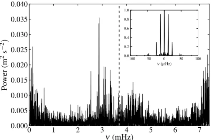
The power spectrum, calculated using the measurement un-certainties as weights, is shown in Fig. 2. The spectral win-dow W, which is the Fourier transform of the observing winwin-dow, w(t) = ! δ(t − ti) (with tithe mid-exposure time of the ith expo-sure), is shown in the inset of Fig.2. Strong aliases caused by the daily gaps appear on both sides of the central peak at multiples of ±11.57 µHz. The power spectrum shows a clear excess around 3 mHz that is characteristic of solar-like oscillations, reaching ∼0.04 m2s−2(corresponding to amplitudes ∼20 cm s−1).
The median sampling time was 135.0 s, including the read-out (∼22.6 s). This leads to an equivalent Nyquist frequency of 3.7 mHz. In Fig.2, we clearly see a steep rise in power at 7 mHz, corresponding to the folded low-frequency increase. This also causes the bump that appears between 3.7 mHz and ∼5.5 mHz, which is an alias of the oscillation spectrum.
The asymptotic relation for high-order p modes is νn,l = (n + l/2 + %s)∆ν, where νn,l is the frequency of the mode with radial order n and angular degree l, the average large separation ∆ν and a surface phase offset %s(Tassoul 1980). There is a peri-odicity of ∆ν/2 in the frequency distribution, implying that there will be a local maximum at this value in the autocorrelation func-tion (ACF) of the signal y(t), defined by Ryy(τ) = E[y∗(t)y(t +τ)] (where E is the expectation value and y∗the complex conjugate of y). The ACF for 18 Sco is shown in Fig.3. Since the sig-nal is irregularly sampled with daily gaps, it was computed by applying the Wiener-Khinchine theorem.
The large separation estimator is thus simply ˜
∆ν = 2× [argmax(Ryy∗ H)]−1,
t∈T (1)
1 An attempt to reduce the daily aliases, with simultaneous observations on SOPHIE (Observatoire de Haute-Provence, run ID: 09A.PNPS.THEA), was unfortunately plagued by bad weather.
Fig. 2.Power spectrum of 18 Sco, evaluated using a weighted Lomb-Scargle “periodogram”. The vertical grey dashed line marks the loca-tion of the equivalent Nyquist frequency. The inset shows the spectral window W, normalized to its maximum.
where T is the domain in which we search for this maxi-mum, which we set at T = [13 000, 25 000] s (i.e. in the fre-quency range 40–80 µHz), and H the Fourier transform of a fil-ter h(ν) that truncates the power spectrum. Indeed, only the range 1500–3700 µHz is considered when computing (using an FFT algorithm) the Fourier transform of the spectrum. We used zero-padding to ensure that the ACF was evaluated at points separated by an “equivalent frequency resolution” ∼0.01 µHz. As noted by Roxburgh(2009), the width of h(ν) affects the localization of ˜∆ν, which is a limitation of the method.
The next step is to obtain information about the statistical properties of the estimator ˜∆ν that accounts for the noise in the data. We can write
y = x + ε, (2)
where y = [y0, . . . , yN] are the measured values of the radial ve-locity at times t0, . . . ,tN, x = [x0. . . ,xN] are the true values of the radial velocity and ε = [ε0, . . . , εN] is a vector gathering the noise contributions from observational errors. Our goal is to es-timate the probability density of ˜∆ν conditional ony, p( ˜∆ν|y). To do so, we used a Monte Carlo approach to error propaga-tion. We assumed that the noise in the data is a series of realiza-tions of independent random variables distributed according to the Gaussian distributions Ni =N(x(ti), σ2i), with the σigiven by the uncertainties on the data. We simulated time series by generating new realizations of the noise distributed according to the Niat each tiand adding them to yi. For each artificial set of data ya, we estimated ˜∆νa.
Our process for generating the artificial data means that it satisfies
ya=y + ε!= x +ε + ε!, (3)
with ε!the artificially generated noise, and ε!and ε both real-izations of the same distribution at time ti. Ideally, one wishes to estimate the large separation from x. One possibility would be to estimate it from several measurements, on different tele-scopes at the same times ti. A second way would be to generate the yafrom a model reproducing the data y, then perturbing the output of this model, rather than the real observations, which is the classical procedure of Monte Carlo estimation of parameters. Unfortunately, the knowledge of ∆ν alone does not permit such a model to be set up.
M. Bazot et al.: The radius and mass of the close solar twin 18 Scorpii derived from asteroseismology and interferometry
Fig. 3. Filtered autocorrelation function for the observed data. The shaded area marks the interval T , in which we searched for the local maximum corresponding to ∆ν/2. F is the Fourier transform.
It thus has to be assumed that this bias will not be too severe, which can be crudely checked graphically with an échelle dia-gram (see Fig.4). Further estimations of the large separations, using individual frequencies, may give us some information on its magnitude. However, the error bars are representative of the error propagation: were we able to correct for the bias induced by random observational noise, we would expect our confidence interval on the large separation to be the same.
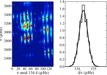
Figure 4 shows the results for our Monte Carlo suite of 10 000 time series. It closely follows a Gaussian distribution with parameters µ = 134.4 µHz and σ = 0.3 µHz. The right panel represents the échelle diagram of the observations using this value for the mean large separation.
3. Interferometry
To measure the angular diameter of 18 Sco, which is expected to only be about 0.7 mas, we used long-baseline interferome-try at visible wavelengths. We used the PAVO beam combiner (Precision Astronomical Visible Observations; Ireland et al. 2008) at the CHARA array (Center for High Angular Resolution Astronomy;ten Brummelaar et al. 2005). We obtained four cal-ibrated sets of observations on 18 July 2009 using the S1-W2 (211 m) baseline.
PAVO records fringes in 38 wavelength channels centred on the R band (λc( 700 nm). The raw data were reduced using the PAVO data analysis pipeline (Ireland et al. in prep.). To enhance the signal-to-noise ratio, the analysis pipeline can average over several wavelength channels, and for 18 Sco we found an opti-mal smoothing width of five channels. Excluding four channels on each end because of edge effects, this resulted in six inde-pendent data points per scan and hence a total of 24 indeinde-pendent visibility measurements for 18 Sco.
Table1lists the three stars we used to calibrate the visibili-ties. We estimated their angular diameters, θ, using the V–K cal-ibration ofKervella et al.(2004). Although the internal precision of this calibration, as well as the uncertainties in the photometry for all three stars, is better than 1%, we assume here conservative uncertainties of 5% for each calibrator (van Belle & van Belle 2005). These incorporate the unknown orientation and expected oblateness in fast rotators (Royer et al. 2002). These were cho-sen to be single stars with predicted diameters at least a factor of two smaller than 18 Sco and to be nearby on the sky (at a sepa-ration d < 10◦). Each of the four scans of 18 Sco was calibrated, using a weighted mean of the calibrators bracketing the scan. All
Fig. 4.Left panel: échelle diagram corresponding to the mean value of ˜
∆ν. Right panel: results from the Monte Carlo experiment. The his-togram shows the distribution of the actual realizations, and the contin-uous line the Gaussian with the corresponding mean and variance.
scans contributing to a bracket were made within a time interval of 15 min. The final calibrated squared-visibility measurements are shown in Fig.5as a function of spatial frequency.
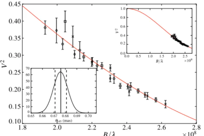
To determine the angular diameter, corrected for limb dark-ening, we fitted the following model to the data (Hanbury Brown et al. 1974): V = " 1 − µλ 2 + µλ 3 #−1$ (1 − µλ) J1(x) x + µλ(π/2) 1/2J3/2(x) x3/2 % (4) with x = πBθLDλ−1. Here, V is the visibility, µλthe linear limb-darkening coefficient, Jn(x) the nth order Bessel function, B the projected baseline, θLDthe limb-darkened angular diameter, and λ the wavelength at which the observations were done. In our analysis, we used µλ= 0.607± 0.012, which is interpolated at the Teff, log g, and metallicity of 18 Sco in the R-filter given in the catalog ofClaret(2000). For all wavelength channels, we assumed an absolute error of 5 nm (∼0.5%).
Interferometric measurements are often dominated by sys-tematic errors and therefore require a careful analysis of all er-ror sources. To arrive at realistic uncertainties for the angular diameter, we performed a series of 104Monte Carlo simulations as follow. For each simulation, we drew realizations from the observed values (assuming they correspond to the parameters of Gaussian distributions) for the calibrator angular diameters, limb darkening coefficient, and wavelength channels. With these pa-rameters we then calibrated the raw visibility measurements and fit the angular diameter θLDto the calibrated data using a least-squares minimization algorithm. Finally, we generated for each simulation a random sample of 200 normally distributed points with a mean corresponding to the fitted diameter and a stan-dard deviation corresponding to the formal uncertainty (scaled so that χ2= 1) of the fit. For each Monte-Carlo simulation these 200 points were stored to make up the final distribution con-taining 2 × 10⁶ points. This procedure was carried out for all independent measurements in our data.
The resulting distribution for the diameter of 18 Sco is shown in Fig. 5, along with the best-fitting model. The mean and standard deviation of this distribution yield θLD = 0.6759± 0.0062 mas. Combined with the Hipparcos parallax of 71.94 ± 0.37 mas (van Leeuwen 2007), we find the radius of 18 Sco to be R/R"= 1.010± 0.009. We conclude that the radius of 18 Sco is the same as the Sun, within an uncertainty of 0.9%.
A&A 526, L4 (2011)
Fig. 5.Calibrated squared visibilities for 18 Sco. The red line represents the best model. Each symbol type corresponds to one scan, the visibility averaged over five wavelength channels. Upper-right inset: same model represented on a larger scale. Lower-left inset: distribution for angular diameter (mean and standard deviation represented by vertical lines). Table 1. Properties of the calibrators used for 18 Sco.
Star Va Kb Sp. Type θ(mas) d(deg)
HD 145607 5.435 5.052 A4V 0.343 ± 0.017 0.9
HD 145788 6.255 5.737 A1V 0.256 ± 0.013 4.2
HD 147550 6.245 5.957 B9V 0.233 ± 0.012 6.5
Notes. (a) http://simbad.u-strasbg.fr/simbad/ (b) http://
www.ipac.caltech.edu/2mass/
4. Mass of 18 Sco
Gough(1990) pointed out that the homology relation:
∆ν∝ M1/2R−3/2, (5)
holds for main-sequence stars even outside the zero-age main sequence. Other studies have confirmed this picture (e.g.,Stello et al. 2009).
Applying the ACF method described above to a one-year BiSON time series of the Sun (Broomhall et al. 2009, and references therein), we found the solar large separation to be 135.229 ± 0.003 µHz. With our radius measurement this gives a mass M = 1.02 ± 0.03 M" for 18 Sco. The agreement is good with the published estimates derived from indirect meth-ods, such as comparison between spectro- or photometric obser-vations and stellar evolutionary tracks (Valenti & Fischer 2005; Meléndez & Ramírez 2007; Takeda et al. 2007; Sousa et al. 2008;do Nascimento et al. 2009).
The assumption of homology is in general well-supported by the comparison to models. Considering a small departure from it in the form ∆ν ∝ (1 + c)M1/2R−3/2(with c + 1, being a function of the structure of the star), we then have for a scaling relative to the Sun, c = (∆ν/∆ν")(M/M")1/2(R/R
")−3/2− 1. For stellar ages characteristics of those quoted for 18 Sco (the dependence on the mass and the metallicity being weak), this quantity may contribute to an additional ∼0.2%–0.4% on the total error on the mass.
The impact of filtering the ACF is not completely negligi-ble, and if we vary the lower limit of T , between 1500 µHz and 2000 µHz, the final estimate may vary by ∼0.01 M", emphasiz-ing the need for individual frequency measurements.
5. Conclusion
We presented the first asteroseismic and interferometric mea-surements for the solar twin 18 Sco. These allowed us to esti-mate a mass for this star independent of the previous spectro-photometric studies, which are still being confirmed. This work shows the possibilities offered by asteroseismology, even from a ground-based single site, and iby nterferometry. Our results con-firm that 18 Sco is remarkably similar to the Sun in both radius and mass.
The next step will involve measuring the individual oscil-lation frequencies and performing full modelling using all the available observations. It will hopefully reduce the uncertainty on the estimated age, improving our knowledge of the physical state of 18 Sco (do Nascimento et al. 2009). This will provide a more precise picture of its interior and give information on the depth of its external convective zone (Monteiro et al. 2000), which is necessary if one wishes to study its magnetic activity cycle (Petit et al. 2008).
Acknowledgements. This work was supported by grants SFRH/BPD/47994/2008, AST/098754/2008, and PTDC/CTE-AST/66181/2006, from FCT/MCTES and FEDER, Portugal. This research was supported by the Australian Research Council (project number DP0878674). Access to CHARA was funded by the AMRFP (grant 09/10-O-02), supported by the Commonwealth of Australia under the International Science Linkages programme. The CHARA Array is owned by Georgia State University. Additional funding for the CHARA Array is provided by the National Science Foundation under grant AST09-08253, by the W. M. Keck Foundation, and the NASA Exoplanet Science Center.
References
Broomhall, A., Chaplin, W. J., Davies, G. R., et al. 2009, MNRAS, 396, L100 Cayrel de Strobel, G., Knowles, N., Hernandez, G., & Bentolila, C. 1981, A&A,
94, 1
Claret, A. 2000, A&A, 363, 1081
Creevey, O. L., Monteiro, M. J. P. F. G., Metcalfe, T. S., et al. 2007, ApJ, 659, 616
Cunha, M. S., Aerts, C., Christensen-Dalsgaard, J., et al. 2007, A&A Rev., 14, 217
do Nascimento, Jr., J. D., Castro, M., Meléndez, J., et al. 2009, A&A, 501, 687 Gough, D. O. 1990, in Astrophysics: Recent Progress and Future Possibilities,
ed. B. Gustafsson, & P. E. Nissen, 13
Hanbury Brown, R., Davis, J., Lake, R. J. W., & Thompson, R. J. 1974, MNRAS, 167, 475
Ireland, M. J., Mérand, A., ten Brummelaar, T. A., et al. 2008, in Optical and Infrared Interferometry, Proc. SPIE, 7013, 701324
Kervella, P., Thévenin, F., Di Folco, E., & Ségransan, D. 2004, A&A, 426, 297 Mayor, M., Pepe, F., Queloz, D., et al. 2003, The Messenger, 114, 20 Meléndez, J., & Ramírez, I. 2007, ApJ, 669, L89
Meléndez, J., Dodds-Eden, K., & Robles, J. A. 2006, ApJ, 641, L133 Meléndez, J., Asplund, M., Gustafsson, B., & Yong, D. 2009, ApJ, 704, L66 Monteiro, M. J. P. F. G., Christensen-Dalsgaard, J., & Thompson, M. J. 2000,
MNRAS, 316, 165
North, J. R., Davis, J., Bedding, T. R., et al. 2007, MNRAS, 380, L80 Petit, P., Dintrans, B., Solanki, S. K., et al. 2008, MNRAS, 388, 80 Ramírez, I., Meléndez, J., & Asplund, M. 2009, A&A, 508, L17 Roxburgh, I. W. 2009, A&A, 506, 435
Royer, F., Grenier, S., Baylac, M., Gómez, A. E., & Zorec, J. 2002, A&A, 393, 897
Sousa, S. G., Santos, N. C., Mayor, M., et al. 2008, A&A, 487, 373
Stello, D., Chaplin, W. J., Basu, S., Elsworth, Y., & Bedding, T. R. 2009, MNRAS, 400, L80
Takeda, Y., & Tajitsu, A. 2009, PASJ, 61, 471
Takeda, Y., Kawanomoto, S., Honda, S., Ando, H., & Sakurai, T. 2007, A&A, 468, 663
Tassoul, M. 1980, ApJS, 43, 469
ten Brummelaar, T. A., McAlister, H. A., Ridgway, S. T., et al. 2005, ApJ, 628, 453
Valenti, J. A., & Fischer, D. A. 2005, ApJS, 159, 141 van Belle, G. T., & van Belle, G. 2005, PASP, 117, 1263
van Leeuwen, F. 2007, Hipparcos, the New Reduction of the Raw Data, Ap&SS Library, 350,