Hybrid modeling of aboveground biomass carbon using disturbance history over large areas of boreal forest in eastern Canada

Hybrid modeling of aboveground biomass carbon

using disturbance history over large areas of boreal

forest in eastern Canada

Thèse

Dinesh Babu Irulappa Pillai Vijayakumar

Doctorat en sciences forestières

Philosophiae doctor (Ph.D.)

Québec, Canada

iii

Résumé

Le feu joue un rôle important dans la succession de la forêt boréale du nord-est de l’Amérique et le temps depuis le dernier feu (TDF) devrait être utile pour prédire la distribution spatiale du carbone. Les deux premiers objectifs de cette thèse sont: (1) la spatialisation du TDF pour une vaste région de forêt boréale de l'est du Canada (217,000 km2_{) et (2) la prédiction du carbone de la biomasse aérienne (CBA) à l’aide}

du TDF à une échelle liée aux perturbations par le feu.

Un modèle non paramétrique a d’abord été développé pour prédire le TDF à partir d’historiques de feu, des données d'inventaire et climatiques à une échelle de 2 km2_{. Cette échelle correspond à la superficie}

minimale d’un feu pour être inclus dans la base de données canadienne des grands feux. Nous avons trouvé un ajustement substantiel à l’échelle de la région d’étude et à celle de paysages régionaux, mais la précision est restée faible à l’échelle de cellules individuelles de 2 km2_.

Une modélisation hiérarchique a ensuite été développée pour spatialiser le CBA des placettes d’inventaire à la même échelle de 2 km2_{. Les proportions des classes de densité du couvert étaient les}

variables les plus importantes pour prédire le CBA. Le CBA co-variait également avec la vitesse de récupération du couvert au travers de laquelle le TDF intervient indirectement.

Finalement, nous avons comparé des estimations de CBA obtenues par télédétection satellitaire avec celles obtenues précédemment. Les résultats indiquent que les proportions des classes de densité du couvert et des types de dépôts ainsi que le TDF pourraient servir comme variables auxiliaires pour augmenter substantiellement la précision des estimés de CBA par télédétection.

Les résultats de cette étude ont montré: 1) l'importance d’allonger la profondeur temporelle des historiques de feu pour donner une meilleure perspective des changements actuels du régime de feu; 2) l'importance d'intégrer l’information sur la reprise du couvert après feu aux courbes de rendement de CBA dans les modèles de bilan de carbone; et 3) l'importance de l'historique des feux et de la récupération de la végétation pour améliorer la précision de la cartographie de la biomasse à partir de la télédétection.

v

Abstract

Fire is as a main succession driver in northeastern American boreal forests and time since last fire (TSLF) is seen as a useful covariate to infer the spatial variation of carbon. The first two objectives of this thesis are: (1) to elaborate a TSLF map over an extensive region in boreal forests of eastern Canada (217,000 km2_{) and (2) to predict aboveground carbon biomass (ABC) as a function of TSLF at a scale related to fire}

disturbances.

A non-parametric model was first developed to predict TSLF using historical records of fire, forest inventory data and climate data at a 2-km2 _{scale. Two kilometer square is the minimum size for fires to be}

considered important enough and included in the Canadian large fire database. Overall, we found a substantial agreement at the scale of both the study area and landscape units, but the accuracy remained fairly low at the scale of individual 2-km2 _cells.

A hierarchical modeling approach is then presented for scaling-up ABC from inventory plots to the same 2 km2 _{scale. The proportions of cover density classes were the most important variables to predict ABC.}

ABC was also related to the speed of post-fire canopy recovery through which TSLF acts indirectly upon ABC.

Finally, we compared remote sensing based aboveground biomass estimates with our inventory based estimates to provide insights on improving their accuracy. The results indicated again that abundances of canopy cover density classes of surficial deposits, and TSLF may serve as ancillary variables for improving substantially the accuracy of remotely sensed biomass estimates.

The study results have shown: 1) the importance of lengthening the historical records of fire records to provide a better perspective of the actual changes of fire regime; 2) the importance of incorporating post-fire canopy recovery information together with ABC yield curves in carbon budget models at a spatial scale related to fire disturbances; 3) the importance of adding disturbance history and vegetation recovery trends with remote sensing reflectance data to improve accuracy for biomass mapping

vii

Table of contents

Résumé ... iii

Abstract ... v

Table of contents ... vii

List of Tables ... xi

List of Figures ... xiii

Acknowledgements ... xvii

Preface ... xix

1. General Introduction ... 1

1.01 What is a forest carbon stock? ... 1

1.02 Carbon stocks in Canadian boreal ecosystems ... 1

1.03 Dynamics of the black spruce forest ... 4

1.04 Why map TSLF? ... 5

1.05 Research problem and motivation ... 5

1.06 Objectives ... 7

1.07 References ... 9

Chapter 1: Lengthening the historical records of fire history over large areas of boreal forest

2.

in eastern Canada using empirical relationships ... 15

2.01 Abstract ... 16

2.02 Introduction ... 17

2.03 Methods ... 18

2.03.01 Study Area ... 18

2.03.02 Characterization of study units ... 19

2.03.03 Modelling TSLF ... 22

2.03.04 TSLF extrapolation to the entire study area ... 26

2.03.05 Relating forest composition with past disturbances at the landscape scale ... 26

2.04 Results ... 27

2.04.01 Accuracy of TSLF models ... 27

2.04.02 Temporal changes in the decadal burn rate during the 20

th

_{century ... 29}

2.04.03 Forest composition in relation to fire regime as derived from the TSLF map ... 29

2.05 Discussion ... 31

viii

2.05.02 Interpretation of TSLF predictors ... 32

2.05.03 Impacts of spatial scale on TSLF modelling ... 32

2.05.04 Temporal changes in regional burn rate ... 33

2.05.05 Management and conservation implications ... 33

2.06 Conclusion... 33

2.07 Acknowledgements ... 34

2.08 References ... 35

2.09 Supplementary material ... 41

Chapter 2: Cover density recovery after fire disturbance controls landscape aboveground

3.

biomass carbon in the boreal forest of eastern Canada ... 45

3.01 Abstract ... 46

3.02 Introduction... 47

3.03 Material and Methods ... 48

3.03.01 Study region ... 48

3.03.02 Datasets and study units ... 49

3.03.03 Scaling framework... 52

3.03.04 Quantifying information loss due to scaling-up ... 54

3.03.05 Result synthesis and visualization... 54

3.04 Results ... 55

3.04.01 Estimation of aboveground biomass carbon ... 55

3.04.02 Variation of cover density and ABC yield curves at a regional scale ... 57

3.05 Discussion ... 61

3.05.01 Interpretation of ABC predictors at plot level ... 61

3.05.02 Relationship between ABC and TSLF at the 2-km

2

_{scale ... 61}

3.05.03 Comparing accuracy with previous studies ... 62

3.05.04 Implications for C budget modelling ... 62

3.06 Conclusion... 63

3.07 Acknowledgements ... 64

3.08 References ... 65

Chapter 3: Fire disturbance history improves the consistency of remotely sensed

4.

aboveground biomass estimates for boreal forests in eastern Canada ... 73

4.01 Abstract ... 74

4.02 Introduction... 75

ix

4.03.01 Study area ... 78

4.03.02 Estimation of AGB based on inventory data ... 79

4.03.03 Estimations of AGB from remote sensing data ... 80

4.03.04 Comparison of biomass maps ... 82

4.04 Results ... 84

4.04.01 Estimation of AGB using GLAS canopy height data ... 84

4.04.02 Spatial distribution and covariation of remotely sensed and inventory based

biomass estimates ... 85

4.04.03 Spatial analysis of differences between inventory and remotely sensed biomass

estimates ... 88

4.04.04 Detecting potential ancillary variables for remotely sensed AGB estimation ... 88

4.04.05 AGB yield curves with remotely sensed products ... 89

4.05 Discussion ... 94

4.05.01 Interpreting covariation and spatial distribution of biomass estimates ... 94

4.05.02 Consistency of results among comparable studies ... 96

4.05.03 Potential ancillary variables for remotely sensed AGB estimation ... 96

4.06 Conclusion ... 98

4. 07 Acknowledgements ... 98

4.08 References ... 100

4.09 Supplementary material ... 108

5. General Conclusion ... 111

5.01 References ... 113

xi

List of Tables

Table 2-1. List of explanatory variables considered for the training of the random forest models

... .21

Table 2-2. Sources used to generate the response variable for the training dataset for the

random forest TSLF models ... 24

Table 2-3. Average proportions of tree species by vegetation cluster after a clustering analysis to

explain the homogeneity of landscape units by vegetation composition. Species names are

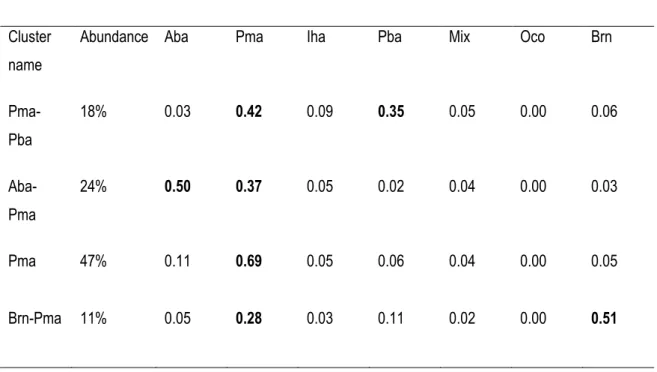
provided in Table 2.1. Bold numbers indicate the dominant species ... 30

Table 3-1. Mean proportions of the relative abundances of surficial deposits classes: very

abundant, very coarse (VAVC); abundant, coarse (AC); rock (ROC); and organic (ORG) (Mansuy

et al., 2010), and the means of degree-days by each cluster, which were used to explain

homogeneity of the landscape units. Bold numbers indicate the maximum value of variables that

were used for clustering (values are normalized). ... 58

Table 4-1. List of explanatory variables used in estimating AGB ... 83

Table 4-2. Pearson correlations between each of MODIS, GLAS, ASAR and inventory based

AGB estimates after accounting for spatial autocorrelation*. ... 86

xiii

List of Figures

Figure 2.1. Location of study area (outlined in dark black) and fire history maps (numbered

grayed areas, refer to Table 2.2). Inventory plots used for the training of the TSLF models are not

shown. ... 19

Figure 2.2. For the top six variables (Table 2.1), ranked by the random forest models for the

classification of 2-km

2

_{cells into TSLF ≤ 120 years and TSLF > 120 years, (a) normalized mean}

decrease in Gini coefficient, and (b) normalized mean decrease in mean square error in

predicted cell-level TSLF for cells in which TSLF is predicted to be less than 120 years; c)

density plot of observed vs predicted year of stand origin for cells for which TSLF is predicted ≤

120 years; d) box-and-whisker plots of margins of error for predicted TSLF values grouped by

decade class; e) Decadal burn rates between 1880 and 2000 for the study region (dark grey:

burn rate correction due to survival analyses, light grey: highest values of burn rate, hatching:

burn rates between 1970 and 2000). ... 28

Figure 2.3. Map of predicted time since last fire by decade class (between1880 and 2000). The

map was generalized by aggregating 2-km

2

_{cells of identical period of fire activity (1880-1920,}

1920-1940, 1940-1970 and 1970-2000) and by removing any object smaller than 4 km

2

_{. ... 29}

Figure 2.4. a) Vegetation map of landscape units (ecological districts) derived from a cluster

analysis based on species abundance. Average proportions of species and names for each

cluster are presented in Table 2.3; b) box-and-whisker plots of mean time since last fire by

ecological district across the vegetation clusters; c) frequency of 2-km

2

_{cells with a TSLF value}

above or below 120 years by vegetation cluster. ... 31

Figure 3.1. Panel a) Location of the study area (dark outline) with training areas for which time-

since-last-fire was available from published studies. Panel b) Distribution of forest inventory plots

used in the analysis. ... 51

Figure 3.2. Top six variables ranked by the random forest models for the prediction of ABC at

plot level (a) and at scale of 2-km

2

_{cells (d). Density plot of estimated ABC vs predicted ABC at}

plot level (b) and at 2-km

2

_{scale (e). c) Map of ABC predicted with RF modelling at the scale of 2}

xiv

Figure 3.3. (a) Box-and-whisker plots of the coefficient of variation of residual variance for

individual 2-km

2

_{cells as a function of the number of repetitions of RF model training for ABC}

prediction. (b) Density plot of estimated vs predicted ABC values at 2-km

2

_{scale when variability}

of predicted values at SIFORT tile centroid level is considered for ABC predictions. (c) Density

plot of predicted values of ABC at 2-km

2

_{scale when variability of predicted values at SIFORT tile}

centroid level is considered (B) or not (A). ... 57

Figure 3.4. Cluster map (“organic,” “coarse,” and “typical” zones) of ecological districts based on

centroid degree-days and their relative abundances of marginal surficial deposit groups (organic,

stony and coarse-textured, and rock surficial deposits). ... 59

Figure 3.5. Box-and-whisker plots of ABC as a function of time-since-last-fire at 2-km

2

_{scale cells}

in “organic” (a), “coarse” (b), and “typical” (c) zones; box-and-whisker plots of the abundance of

closed-density cover (> 81%, 61-80%, and 41-60%) as a function of time-since-last-fire for 2-km

2

scale cells “organic” (d), “coarse” (e), and “typical” (f) zones. ... 60

Figure 4.1. General flow diagram ... 78

Figure 4.2. Locations of the study area (dark outline) and training datasets (grey areas) from the

published studies. ... 79

Figure 4.3. Top six variables ranked by a random forest model for the estimation of AGB based

on observed canopy height at plot level (a); (b) density plot of estimated vs predicted AGB by the

model based on observed canopy height at plot level ... 85

Figure 4.4. Maps of AGB at the scale of 2 km

2

_{based on: inventory data (a); MODIS data}

obtained from Beaudoin et al. (2014) (b); GLAS data (c); ASAR data obtained from Thurner et al.

(2014) (d) ... 87

Figure 4.5 Top-six variables ranked by RF models used to explain the differences observed

between remotely sensed and inventory based AGB estimates with relative frequencies of

SIFORT attributes (Table 4.1) and observed TSLF: MODIS (a); GLAS (b); and ASAR (c); density

plots of observed vs predicted AGB differences between inventories based and remotely sensed

AGB estimates: MODIS (d), GLAS (e), and ASAR data (f). ... 90

xv

Figure 4.6. Box-and-whisker plots of differences observed between inventory based AGB

estimates and biomass estimates of MODIS (a), GLAS (b), and ASAR (c), regrouped by

abundance classes of canopy closed cover density. ... 91

Figure 4.7. Top-six variables ranked by RF models used to explain the differences observed

between remotely sensed and inventory based AGB estimates when abundances of cover

canopy density classes are removed from the list of potential explanatory variables: MODIS, (a);

GLAS, (b); and ASAR, (c); density plots of observed vs predicted AGB differences between

remotely sensed and inventory based AGB estimates: MODIS (d); GLAS (e); and ASAR data (f).

... 92

Figure 4.8. Box-and-whisker plots of AGB estimates based on inventory data (a), MODIS (b),

GLAS (c), and ASAR data (d) as a function of TSLF at the 2-km

2

_{scale. ... 93}

xvii

Acknowledgements

I would like to express my sincere gratitude to my PhD supervisor, Dr. Frédéric Raulier (Professor, Université Laval), who supported me from the initial start of defining my research proposal to the end of this study. I started PhD without any knowledge on boreal forests and today I have learned many things from my PhD supervisor with his critical and helpful comments.

I would like to thank my co-supervisor Dr. Pierre Bernier (senior scientist, Canadian Forest Service, Laurentian Forestry Center) for guiding me in my study and helping a lot while writing manuscripts. I would like to thank Dr. Sylvie Gauthier (senior scientist, Canadian Forest Service, Laurentian Forestry Center), Dr. Yves Bergeron (Chaire industrielle CRSNG-UQAT-UQAM en aménagement forestier durable, Université du Québec en Abitibi-Témiscamingue, UQAT) and Dr. David Pothier (Professor, Université Laval) for graciously providing fire history maps. They also helped for writing manuscripts. I also thank Dr. Dominic Cyr, Dr. Héloïse Le Goff, Dr. Annie-Claude Bélisle and Daniel Lesieur for their fire history maps. Without these precious and expensive data, this study would not have been possible. Thanks a lot everybody!!!

I also thank Dr. David Paré (senior scientist, Canadian Forest Service, Laurentian Forestry Center) who was part of my doctoral committee for very useful comments on this study and particularly chapter 2. I am very much grateful to Hakim Ouzenou (Research professional, Université Laval) for helping with SAS programming and also for French translation. I would also like to appreciate Dr. Steven cumming (Professor, Université Laval) and Dr. Alain Leduc (Professor, Université du Québec à Montréal) for their comments to improve the final version of this thesis.

I also thank Dr. Narayan Prasad Dhital, Dr. Kenneth Agbesi Anyomi, Dr. Julien Beguin, Guillaume Cyr, Baburam and Gina for social gathering and discussions beyond the lab work.

xix

Preface

This thesis consists of five sections; General Introduction, Chapter 1, Chapter 2, Chapter 3, and General Conclusion.

Chapter 1 to 3 correspond to the following (published, submitted or under preparation) articles:

1) Irulappa Pillai Vijayakumar, D.B., Raulier, F., Bernier, P. Y., Gauthier, S., Bergeron, Y., & Pothier, D. 2015. Lengthening the historical records of fire history over large areas of boreal forest in eastern Canada using empirical relationships. Forest Ecology and Management, 347, 30-39.

2) Irulappa Pillai Vijayakumar, D.B., Raulier, F., Bernier, P. Y., Paré, D., Gauthier, S., Bergeron, Y., & Pothier, D. 2016. Cover density recovery after fire disturbance controls landscape aboveground biomass carbon in the boreal forest of eastern Canada. Forest Ecology and Management, 360, 170–180.

3) Irulappa Pillai Vijayakumar, D.B., Raulier, F., Bernier, P. Y., Gauthier, S., Bergeron, Y., & Pothier, D. Fire disturbance history improves the consistency of remotely sensed aboveground biomass estimates for boreal forests in eastern Canada (Manuscript under preparation)

Forest inventory data, SIFORT and SOPFEU fire polygons data for this study were provided by Ministère de la Forêt, de la Faune et des Parcs. Dr. Sylvie Gauthier (senior scientist, Canadian Forest Service, Laurentian Forestry Center), Dr. Yves Bergeron (Chaire industrielle CRSNG-UQAT-UQAM en aménagement forestier durable, Université du Québec en Abitibi-Témiscamingue, UQAT) and Dr. David Pothier (Professor, Université Laval) provided fire history maps for this study. Dr. David Paré (senior scientist, Canadian Forest Service, Laurentian Forestry Center) was part of our project, and provided suggestions and comments on this study.

1

1. General Introduction

1.01 What is a forest carbon stock?

The carbon cycle can be defined as “the constant movement of carbon from the land and water through the atmosphere and living organisms” (Natural Resources Canada, 2015). Carbon is an abundant element that is a constituent of all terrestrial life. Several reservoirs make up the carbon (C) cycle. Among these, forests cover ~32 million km2 _{(Hansen et al., 2010) in tropical, temperate, and boreal biomes and}

play an important role in tempering terrestrial climatic variations (Schimel, 1995). “A forest ecosystem includes the living organisms of the forest, and it extends vertically upward into the atmospheric layer enveloping forest canopies and downward to the lowest soil layers affected by roots and biotic processes” (Waring and Running, 2007). In forest ecosystems, C begins its cycle through photosynthesis. Atmospheric C is transformed into carbohydrates using solar energy and water. Trees release part of their carbohydrates through respiration and store another part in their biomass (foliage, stems, and roots) which constitute carbon stocks. Tree biomass contains approximately 50% carbon. Through senescence, litterfall and mortality, organic matter accumulates on soil and is either released during its decomposition by biological organisms or accumulates in soil carbon stocks.

Aboveground biomass (AGB) is an important biophysical parameter for understanding terrestrial carbon stocks dynamics (Houghton et al., 2009). AGB corresponds to the total oven-dried biological material or mass present above the soil including stump, stem, branches, and foliage in a given area at a given time. Most of C stocks are in the tropical forests (55% of total C stocks, including in soil to 1m depth and live biomass), whereas 32% of C stock is present in boreal forests (Pan et al., 2011). The allocation of C stocked between the vegetation and soils of all ecosystems varies with latitude (Dixon et al., 1994). For example, boreal ecosystems store large amount of the carbon in the soils rather than in vegetation, i.e., 84% of the carbon lies in soil organic matter and the remaining in the living biomass (Malhi et al., 1999). Deforestation is the main driver of carbon dynamics in tropical forests, whereas in boreal forests, natural disturbance and harvesting are the most prominent disturbances that influence carbon stocks (Houghton, 2005). With an increasing interest in the effects of human alteration on the global carbon cycle, knowledge of forest carbon content on a regional and extended-time scale becomes important (Houghton, 2003).

1.02 Carbon stocks in Canadian boreal ecosystems

The boreal forest consists of coniferous and deciduous tree species that covers 11% of the earth's terrestrial surface (Bonan and Shugart, 1989). Twelve percent of the global boreal biome is found within Canada (Burton et al., 2010). Canada’s forests therefore play a role in global C cycle for its size and enormous quantity of C stored in vegetation, deep soil, and permafrost pools (Natural Resources Canada, 2012). Canada’s managed forest stocks about 28 Pg of carbon in biomass, dead organic matter and soil

2

pools (Kurz et al., 2013). Improving accuracy in quantifying carbon stocks with an enhanced knowledge of the boreal ecosystems is a key objective of carbon science in Canada (Natural Resources Canada, 2012). Still, capturing spatial variability of carbon stocks at a large scale in the boreal forest remains a challenging issue.

The boreal forests of Canada are the largest supplier of forest products to the world markets (Golden et al., 2011). Intergovernmental panel on climate change (IPCC) recognises that the use of harvested wood products for construction instead of concrete, steel, aluminum and plastic materials could generate carbon emissions reductions (Watson, 2009). The use of forest products for energy also provides a sustainable and renewable resource of energy (Barker, 2007). In recent years, the Canadian forest sector has been facing difficult times and it is in the view of diversifying its markets through the sale of harvest residues and biomass for energy to increase revenue (Paré et al., 2011). To make a profitable forest based products business, it is a responsibility of forest managers to follow an ecosystem-based forest management approach. Ecosystem-based forest management approach is defined as “a management approach that aims to maintain healthy and resilient forest ecosystems by focusing on a reduction of differences between natural and managed landscapes to ensure long term maintenance of ecosystem functions and thereby retain the social and economic benefits they provide to society” (Gauthier et al., 2009). In this approach, the management practices should emulate natural disturbances and maintain biodiversity and forest ecosystem functions (Bergeron et al., 1999). The underlying concept is that species are usually adapted to their natural environmental conditions, including the range of natural variability. This basic concept entails that “past conditions and processes provide a context and the guidance for managing ecological systems today, and that disturbance-driven spatial and temporal variability is a vital attribute of nearly all ecological systems” (Landres et al., 2007). In this context, understanding ecosystem processes and functions including disturbance regimes, is essential to reduce the differences between natural and managed landscapes (Gauthier et al., 2002). This ecosystem-based management approach is based on coarse filter principles. Under a coarse-filter approach, forest management should ensure the conservation of most species through the preservation of habitat diversity (North and Keeton, 2008). At the landscape level, forest age structure (i.e. age class distribution) is targeted within the natural range of variability. Determination of the harvest rate is based on the rate of natural disturbance (Armstrong, 1999). “The closer an ecosystem is managed to allow for natural ecological processes to function, the more successful that management strategy will be” (Elmore and Kauffman, 1994).

Forest carbon cycle is also an important forest ecological process (Landsberg & Sands, 2010). A coarse filter approach should also tend to reduce the differences between carbon storage in managed and natural landscapes (Henschel and Gray, 2007). Stand carbon content is the sum of the organic carbon (C) present in the overstory biomass, organic soil floor (litter, understory bryophytes, and sphagnum peat

3

mosses) and inorganic or mineral layer. The fundamental elements of the stand-level C contents are the tree species composition, size of trees, canopy cover density, understory, litter, including coarse woody debris and soil substrate (Liu et al., 2011). In Canadian boreal forests, natural disturbance such as fire or insect outbreaks and logging influence the forest C pool. Disturbance is defined as “any relatively discrete event in time that disrupts ecosystem, community, or population structure and changes resources, substrate availability or the physical environment” (Kasischke & Stocks, 2000). Natural disturbances alter forest structure and disturb carbon dynamics in ecosystems (Kurz et al., 2008b). They transfer carbon from the living pool biomass to dead coarse woody debris, forest floor litter and subsurface soil pools. Disturbances modify forest soil’s physical and chemical factors and microclimatic environments. They impact forest structure and reset forest succession transfer (Liu et al., 2011). For example, by altering forest structure, fire also controls soil thermal and moisture regimes, and indirectly controls metabolic processes that drive forest succession, photosynthesis and soil microbial processes (Kasischke & Stocks, 2000).

The important processes which are directly linked to sequestration of carbon are; 1) the rate of photosynthesis which is determined by site productivity, species composition, climate and age of the forest (Kurz et al., 2013); and 2) the rate of decomposition of organic matter (Kasischke and Stocks, 2000). These processes are mostly influenced by climate, physiography and soil factors (Banfield et al., 2002). The rate of C accumulation in the biomass pools depends on the temporal scale; on a short time frame, it is a function of the net ecosystem exchange (daily to weekly to yearly) and on a longer time frame, on the dynamics of forest succession (yearly to decadal time scales) (Kasischke & Stocks, 2000). Following a stand replacing disturbance, C stock in boreal forests first gets reduced and then reaches a maximum during intermediate stand ages that depends on the type and intensity of the last stand replacing disturbance and also of post-fire tree regeneration (Kurz et al., 2013). At landscape level, C stocks are therefore determined by the age class distribution that is the proportion of forest area in different age classes. The forest age-class structure is left shifted with predominately young forests in recently disturbed areas, which has a low C density, whereas it reaches a point of maximum C density with a right shifted age class structure (Kurz and Apps, 1999) in infrequently disturbed forests. In this way, C stays for a certain period of time before it escapes the forest ecosystem due to decomposition and respiration processes and natural disturbances. This residence time of carbon is related to the stability of forest ecosystems (Henschel and Gray, 2007). This residence time further conditions the resistance and resilience qualities which are related to the ability of ecosystem to recover from disturbances (Thompson et al., 2009). The quantity of carbon stocks is also an index of forest ecosystem productivity (Simard et al., 2007, Malhi 2012) and timber production (Simard et al., 2007).

4

1.03 Dynamics of the black spruce forest

The black spruce (Picea mariana (Mill.) BSP) - moss forest (closed-crown forest) is the dominant North American boreal ecosystem (De Lafontaine and Payette, 2011), and such a forest in eastern Canada is the focus of this study. These forests make a large belt at the boundary between closed-canopy and open-canopy (taiga) boreal forests. In this ecosystem, fire is a natural driver of the ecological processes (succession) that dictate forest structure and function (Lecomte et al., 2006, Cyr et al., 2007). Disturbances and succession are key ecological processes that structure landscapes as a mosaic of forest stands of different ages and compositions. Natural black spruce stands originate from fire, after killing the previously established trees, developing into even-aged and closed-crown stands (Kneeshaw and Gauthier, 2003). High severity burns release the nutrients from soil organic carbon content supporting the regeneration of black spruce. In the absence of fire after 120-200 years approximately (Rossi et al., 2009), black spruce trees reach maturity and the death and falling of trees create gaps in the canopy (Grandpré et al., 2000; Harper et al., 2006). Long fire return intervals of approximately 300-1000 years in black spruce forest of eastern Canada (Bergeron et al., 2004b; Bouchard et al., 2008) exceed the life expectancy of black spruce and favors the presence of uneven old-aged stands with unbalanced stand structure (Harper et al., 2006; Bouchard et al., 2008). Black spruce stands are able to maintain for thousands of years in the absence of fire (stable state) (Pollock and Payette, 2010). This represents up to 70% of stands of the eastern black spruce-moss forest in the Province of Quebec (Boucher et al., 2003). The age distribution of black spruce stands is therefore highly skewed towards old stands in this ecosystem and has profound influence on the storage of carbon in soils and living biomass.

Forest age distribution has to be considered for the extrapolation of stand-level carbon budgets to landscapes or regions (Kurz et al., 2008b). In these forests, successional changes are related less to tree species succession but more to structural changes (Harper et al., 2005). The replacement of even-aged closed stands to uneven-aged open canopy stands corresponds to a gradual decline in stand productivity, and is followed by a steady-state phase (Garet et al., 2009). In this way, the stand carbon yield curve is slow at first and then rapidly increases before reaching a maximum near canopy closure, and declines when stands become old and then stabilizes or reduces in the absence of fire (Wang et al., 2003, Martin et al., 2005). Thus, the age structure of the stands conditions the size of carbon stocks stored in forest biomass (Kurz et al., 2008). In fact, TSLF is the right temporal variable to explain the long term dynamics of forest age structure in this region, when the mean longevity of the dominant species can be lower than the time elapsed since the last stand-initiating disturbance (Garet et al., 2012) and also to infer successional patterns (Bouchard et al., 2008). In such case, the mean canopy age will underestimate time since last fire. In this region, the empirical relationship existing between mean canopy age and carbon stocks and the use of mean canopy age to comprehend successional patterns may not be valid. TSLF is also the primary determinant of the accumulation of stand biomass and the soil organic carbon layer

5

depth and its distribution (Simard et al., 2007, Pollock and Payette, 2010). For these reasons, generating wall to wall information of TSLF becomes important in this region for the quantification of biomass.

1.04 Why map TSLF?

Producing a map of TSLF allows us to understand long-term relationships between vegetation, fire and climate for analysing the impact of changes in fire regimes on forest composition. Understanding the extent of change in fire regimes due to climate variability can be used to quantify past ecosystem changes and to compute typical fire return intervals. A TSLF map could also help understand the influence of TSLF on carbon stocks at a regional scale and also aid forest managers for finding insights on ecosystem change for natural resources management planning. Biomass maps integrated with TSLF information can help landscape forest managers to devise management strategies for reducing differences in carbon storage between natural and managed landscapes.

Boreal forest productivity is not only under the control of permanent physical factors but also of transient factors related to forest succession, notably species compositional (Anyomi et al., 2014) and stand structural changes (Boucher et al., 2006). These successional traits are linked to TSLF and thus to past fire activity. Furthermore, landscape productivity is related to its forest age structure, not only because stand productivity is related to its age, but also because tree sensitivity to drought events or to the length of growing seasons is related to its age (Girardin et al., 2012). As a result, past fire activity has a role in forest management and conservation plans for enhancing sustainability and also a significant impact on the actual productivity of the forest.

1.05 Research problem and motivation

Mapping TSLF across a large area over a long temporal scale is inherently challenging in heterogeneous forest environments (Morgan et al., 2001). Existing methods employed to provide TSLF information are either temporally or spatially limited. For example, dendroecological sampling (Girardin et al., 2006) and dating may provide TSLF for longer time spans (Bergeron and Brisson, 1990) but are labour intensive and provide only a spatially-coarse representation of past fire activities (Cyr et al., 2010). The delineation of recent fire scars using aerial photographs provides spatial data of recent burns (Gauthier et al., 2002, Le Goff et al., 2007, Bélisle et al., 2011), but the delineation of fire boundaries remains ambiguous (Cyr et al. 2010). A disadvantage of all these methods is that only present standing trees are measured (recent TSLF), and the information is also spatially restricted over time (Niklasson and Granström, 2000). Analysis of charcoal in lake sediments can be used to determine TSLF over much longer periods of time (Carcaillet et al., 2007, Hély et al., 2010, Payette et al., 2012), but gathering the information is costly and remains limited in space (Niklasson and Granström, 2000).

“Time since last fire” requires making the assumption of complete stand replacement (Johnson and Wagner, 1985). This assumption is only partially valid, since burned areas are expected to be

6

heterogeneous, with residual unburned patches and islands that may occupy between none to 17% of a burned area (Perera et al., 2009). Fire severity is also lower at the burn periphery (Epting and Verbyla, 2005). Burn heterogeneity therefore complicates the estimation of the TSLF, but plays an important role for forest succession (Schmiegelow et al., 2006). Estimation of TSLF at a coarse spatial scale could allow circumventing these issues. There are significant relationships between fire records and vegetation composition and structure (as measured from forest inventory maps) that can be exploited to derive TSLF map (Cyr et al., 2010), but such relationships at a large regional scale have yet to be explored. The spatial variations of successional patterns are also a function of drainage (topographic features) and climatic variables (Senici et al., 2010). Therefore, at large spatial scale, existing fire history generated from dendroecological reconstruction, recent fire burns, and aerial photographs could be linked with the present species composition, age class structure (bottom-up level controls), and climatic variations (top-down controls) and then extrapolated to a larger regional landscape.

Fire alone does not account for the spatial variability of C stocks (Houghton, 2005) and there are other environmental factors (e.g., elevation, soil texture and drainage, Banfield et al., 2002). Most carbon budget models (e.g. Kurz et al., 2009, Masera et al., 2003) do not integrate forest successional dynamics with environmental factors to explain the spatial variability of carbon stocks. It is thus necessary to elaborate a model of carbon dynamics that allows estimating the domain of forest age structures and consequently of carbon stocks that can be expected under a natural disturbance regime (Cyr et al., 2009). Yet, the spatial variability of carbon stocks in relation with TSLF at regional and even local landscape levels is still poorly understood due to the limitation of spatially explicit TSLF information and needs to be better quantified (Balshi et al., 2007, 2009). There is also a lack of knowledge on the relative importance of TSLF and forest structural attributes for estimating aboveground biomass carbon (ABC) across a regional scale in the boreal forest to inform carbon budget models.

Existing methods for mapping ABC fall under two main approaches: 1) ground based and 2) remote sensing approaches. We first have focussed on ground based approaches and later on remote sensing approaches. Modelling may be empirical, process-based and hybrid. Both empirical and process-based methods have advantages and disadvantages. We chose a hybrid modelling approach which is the combination of empirical and process-based knowledge to overcome the limitations encountered with both approaches (Landsberg, 2003). Existing ground based methods utilize large scale forest inventory data to estimate biomass using allometric regression equations or biomass expansion factors or remote sensing data coupled with forest inventory data. Remote sensing techniques are based on the correlation between spectral information (intensity of electromagnetic radiation received by the sensor) and biomass estimated from field measurements and allometric equations. These methods are very useful when there is a scarcity of ground plots data. Studies have demonstrated the existence of correlation between spectral reflectance variables (e.g MODIS, Moderate Resolution Spectroradiometer, Muukkonen et al.,

7

2007) or radar backscatter (e.g. ASAR, Advanced Synthetic Aperture Radar, Thurner et al., 2014) with above ground biomass (AGB). However, these methods are limited in estimating biomass in regions of high biomass, especially when the canopy is closed (Turner et al., 1999). Moreover, the relationship between single date reflectance data and AGB is weak under high leaf area and complex canopy conditions (Pflumagher et al., 2014). On the other hand, LiDAR (light detection and ranging, e.g Geoscience Laser Altimeter System, GLAS) active remote sensing systems, estimate canopy height and vertical structure of the forests directly by determining distance between the sensor and target through obtaining the time between the emission pulse of laser light from the sensor and signal received back in the instrument after reflecting off from the forest canopy and ground (Lefsky et al., 2002). Factors, such as data saturation, mixed pixels, complex biophysical environments, the selection of remote sensing variables, and the modelling approaches all affect AGB accuracy (Lu, 2006). Recent studies of comparing biomass maps from GLAS and MODIS in tropical forests indicated a need to improve their accuracy (Hill et al., 2013, Mitchard et al., 2014). Comparing biomass estimates from remote sensing data with inventory based estimates may therefore allow us to find potential ancillary variables to overcome the problems of saturation signal. Here AGB was used instead of ABC, because AGB maps based on remote sensing data for the area of interest were already available (e.g. Beaudoin et al., 2014, Thurner et al., 2014).

1.06 Objectives

The three objectives of this research are:

1) To map TSLF over large areas of boreal forest at a regional scale by generalizing the empirical relationships that exist between the historical records of fire, forest inventory data, and biophysical setting of the landscape.

2) To predict the spatial variability of ABC as a function of stand and environmental variables across the landscape at a regional scale, and to determine the contribution of TSLF to the predictive model.

3) To explain the spatial variation in AGB differences derived from different remote sensing data (MODIS, GLAS and ASAR) and an AGB model based on ground-inventory data on a large area of boreal forest.

We have chosen the Quebec black spruce-moss commercial forest (area, 217,000 km2_{) for its rich}

information on fire history maps and ground inventory plots, thus serving as a useful training area to map TSLF and further allow us to link aboveground carbon biomass in relation with TSLF. Based on these three objectives, we tailored three chapters for this research in the form of articles published in, submitted

8

to or in preparation for peer reviewed scientific journals. The texts follow the format required for a scientific journal (Forest Ecology and Management).

Chapter 1- Lengthening the historical records of fire history over large areas of boreal forest in eastern Canada using empirical relationships

Chapter 2- Cover density recovery after fire disturbance controls landscape aboveground biomass carbon in the boreal forest of eastern Canada

Chapter 3- Fire disturbance history improves the consistency of remotely sensed aboveground biomass estimates for boreal forests in eastern Canada

9

1.07 References

Anyomi, K. A., Raulier, F., Bergeron, Y., Mailly, D., & Girardin, M. P. (2014). Spatial and temporal heterogeneity of forest site productivity drivers: a case study within the eastern boreal forests of Canada. Landscape ecology, 29(5), 905-918.

Ali, A. A., O. Blarquez, M. P. Girardin, C. Hély, F. Tinquaut, A. El Guellab, V. Valsecchi, A. Terrier, L. Bremond, A. Genries, S. Gauthier, and Y. Bergeron. 2012. Control of the multimillennial wildfire size in boreal North America by spring climatic conditions. Proceedings of the National Academy of Sciences 109:1–5.

Armstrong, G. W. 1999. A stochastic characterisation of the natural disturbance regime of the boreal mixedwood forest with implications for sustainable forest management. Canadian Journal of Forest Research 29:424–433.

Balshi, M. S., McGuire, A. D., Duffy, P., Flannigan, M., Kicklighter, D. W., & Melillo, J. 2009. Vulnerability of carbon storage in North American boreal forests to wildfires during the 21st century. Global Change Biology, 15(6), 1491-1510.

Balshi, M. S., A. D. McGuire, Q. Zhuang, J. Melillo, D. W. Kicklighter, E. Kasischke, C. Wirth, M. Flannigan, J. Harden, and J. S. Clein. 2007. The role of historical fire disturbance in the carbon dynamics of the pan‐boreal region: A process‐based analysis. Journal of Geophysical Research: Biogeosciences (2005–2012) 112.

Banfield, G. E., J. S. Bhatti, H. Jiang, and M. J. Apps. 2002. Variability in regional scale estimates of carbon stocks in boreal forest ecosystems: results from West-Central Alberta. Forest Ecology and Management 169:15–27.

Beaudoin, A., Bernier, P.Y., Guindon, L., Villemaire, P., Guo, X.J., Stinson, G., Bergeron, T., Magnussen, S., Hall, R.J., 2014. Mapping attributes of Canada’s forests at moderate resolution through kNN and MODIS imagery. Canadian Journal of Forest research 44, 521–532.

Bergeron, Y., and J. Brisson. 1990. Fire Regime in Red Pine Stands at the Northern Limit of the Species’ Range. Ecology 71:1352–1364.

Bergeron, Y., Harvey, B., Leduc, A., Gauthier, S., 1999. Forest management guidelines based on natural disturbance dynamics : Stand- and forest-level considerations. The Forestry Chronicle. 75, 49–54. Bergeron, Y., M. Flannigan, S. Gauthier, A. Leduc, and P. Lefort. 2004. Past, current and future fire frequency in the Canadian boreal forest: implications for sustainable forest management. Ambio: A Journal of the Human Environment 33:356–360.

Bhatti, J. S., M. J. Apps, and H. Jiang. 2002. Influence of nutrients, disturbances and site conditions on carbon stocks along a boreal forest transect in central Canada. Plant and Soil 242:1–14.

Bouchard, M., D. Pothier, and S. Gauthier. 2008. Fire return intervals and tree species succession in the North Shore region of eastern Quebec. Canadian Journal of Forest Research 38:1621–1633.

Boucher, D., S. Gauthier, Grandpré. L. De., 2006. Structural changes in coniferous stands along a chronosequence and a productivity gradient in the northeastern boreal forest of Québec. Ecoscience 13:172–180.

Boucher, D., Grandpré, L. De, Gauthier, S., 2003. Développement d’un outil de classification de la structure des peuplements et comparaison de deux territoires de la pessière à mousses du Québec. The forestry chronicle. 79, 318–328.

10

Bonan, G. B., H. H. Shugart. 1989. Ecological processes in boreal forests. Annual Review of Ecology and Systematics 20:1–28.

Burton, P.J., Bergeron, Y., Bogdanski, B.E.C., Juday, G.P., Carcaillet, C., Bergman, I., Delorme, S., Hornberg, G., Zackrisson, O., 2007. Long-term fire frequency not linked to prehistoric occupations in northern Swedish boreal forest. Ecology, 88(2), 465-477.

Clark, J. S. 1990. Fire and climate change curing the last 750 Yr in northwestern Minnesota. Ecological Monographs 60:135–159.

Cyr, D., S. Gauthier, Y. Bergeron, and C. Carcaillet. 2009. Forest management is driving the eastern North American boreal forest outside its natural range of variability. Frontiers in Ecology and the Environment 7:519–524.

Cyr, D., S. Gauthier, D. A. Etheridge, G. J. Kayahara, and Y. Bergeron. 2010. A simple Bayesian Belief Network for estimating the proportion of old-forest stands in the Clay Belt of Ontario using the provincial forest inventory. Canadian Journal of Forest Research 40:573–584.

De Lafontaine, G., Payette, S., 2011. Shifting zonal patterns of the southern boreal forest in eastern Canada associated with changing fire regime during the Holocene. Quaternary Science Reviews. 30, 867–87

Dixon, R. K., A. M. Solomon, S. Brown, R. A. Houghton, M. C. Trexier, and J. Wisniewski. 1994. Carbon pools and flux of global forest ecosystems. Science 263:185–190.

Eliasson, P., Svensson, M., Olsson, M., & Ågren, G. I. 2013. Forest carbon balances at the landscape scale investigated with the Q model and the CoupModel–Responses to intensified harvests. Forest ecology and management, 290, 67-78.

Elmore, W., and B. Kauffman. 1994. Riparian and watershed systems: Degradation and restoration. Society for Range Management.

Epting ,J., Verbyla, D., 2005. Landscape-level interactions of prefire vegetation, burn severity, and postfire vegetation over a 16-year period in interior Alaska. Canadian Journal of Forest Research 35:1367–1377. Fricker, J. M., H. Y. H. Chen, and J. R. Wang. 2006. Stand age structural dynamics of North American boreal forests and implications for forest management. International Forestry Review 8:395–405.

Gauthier, S., M.-A. Vaillancourt, A. Leduc, D. De Grandpré, L. Kneeshaw, H. Morin, P. Drapeau, and Y. Bergeron. 2009. Forest Ecosystem Management Origins and Foundations. Pages 1–37 Ecosystem Management in the Boreal Forest. Presses de l’ Université du Québec, Québec.

Girardin, M. P., Bergeron, Y., Tardif, J. C., Gauthier, S., Flannigan, M. D., Mudelsee, M., 2006. A 229-year dendroclimatic-inferred record of forest fire activity for the Boreal Shield of Canada. International Journal of Wildland Fire, 15(3), 375-388.

Girardin, M. P., Guo, X. J., Bernier, P. Y., Raulier, F., & Gauthier, S. 2012. Changes in growth of pristine boreal North American forests from 1950 to 2005 driven by landscape demographics and species traits. Biogeosciences, 9(7), 2523-2536.

Golden, D. M., M. A. P. Smith, and S. J. Colombo. 2011. Forest carbon management and carbon trading : A review of Canadian forest options for climate change mitigation. The forestry chronicle 87:625–635. Grandpré, L., Morissette, J., Gauthier, S., 2000. Long-term post-fire changes in the northeastern boreal forest of Quebec. Journal of Vegetation Science. Wiley Online Library. 11, 791–800.

11

Hansen, M. C., Stehman, S. V., Potapov, P. V. 2010. Quantification of global gross forest cover loss. Proceedings of the National Academy of Sciences, 107(19), 8650-8655.

Harden, J. W., Trumbore, S. E., Stocks, B. J., Hirsch, A., Gower, S. T., O'neill, K. P. and Kasischke, E. S. (2000), The role of fire in the boreal carbon budget. Global Change Biology, 6: 174–184.

Harper, K.A., Bergeron, Y., Drapeau, P., Gauthier, S., DeGrandpré, L. 2005. Structural development following fire in black spruce boreal forest. Forest Ecology and Management. 206(1–3): 293–306.

Harper, K.A., Bergeron, Y., Drapeau, P., Gauthier, S., De Grandpré, L., 2006. Changes in spatial pattern of trees and snags during structural development in Picea mariana boreal forests. Journal of Vegetation Science. 17, 625–636.

Henschel, C., Gray, T. 2007. Forest carbon sequestration and avoided emissions. In A background paper

for the Canadian Boreal Initiative/Ivey Foundation Forests and Climate Change Forum, Kananaskis, Alberta. Ivey Foundation, Toronto.

Houghton, R. A. 2003. Why are estimates of the terrestrial carbon balance so different? Global Change Biology 9:500–509.

Houghton, R. A. 2005. Aboveground forest biomass and the global carbon balance. Global Change Biology, 11(6), 945-958.

Hély, C., M. P. Girardin, A. A. Ali, C. Carcaillet, S. Brewer, and Y. Bergeron. 2010. Eastern boreal North American wildfire risk of the past 7000 years: A model-data comparison. Geophysical Research Letters 37:1–6.

Hill, T. C., Williams, M., Bloom, A. A., Mitchard, E. T., Ryan, C. M., 2013. Are inventory based and remotely sensed above-ground biomass estimates consistent? PloS one, 8(9), e74170.

Johnson, E. A., and Wagner. C. E. V., 1985. The theory and use of two fire history models. Canadian Journal of Forest Research 15:214–220.

Kasischke, E. S., Stocks, B. J. (2000). Fire, climate change and carbon cycling in the Boreal Forest. New York: Springer-verlag.

Kasischke, E. S., N. L. Christensen Jr., and B. J. Stocks. 1995. Fire, Global Warming, and the Carbon Balance of Boreal Forests. Ecological Applications 5:437–451.

Kelly, R., M. L. Chipman, P. E. Higuera, I. Stefanova, L. B. Brubaker, and F. S. Hu. 2013. Recent burning of boreal forests exceeds fire regime limits of the past 10,000 years. Proceedings of the National Academy of Sciences .

Kneeshaw, D., Gauthier, S., 2003. Old growth in the boreal forest: A dynamic perspective at the stand and landscape level. Environmental Review. 11, S99–S114.

Kurz, W. A., Apps, M. J., 1999. A 70-year retrospective analysis of carbon fluxes in the Canadian forest sector. Ecological Applications, 9(2), 526-547.

Kurz, W. A., C. C. Dymond, G. Stinson, G. J. Rampley, E. T. Neilson, A. L. Carroll, T. Ebata, and L. Safranyik. 2008a. Mountain pine beetle and forest carbon feedback to climate change. Nature 452:987– 990.

Kurz, W. A., Stinson, G., Rampley, G. J., Dymond, C. C., & Neilson, E. T. 2008b. Risk of natural disturbances makes future contribution of Canada's forests to the global carbon cycle highly uncertain. Proceedings of the National Academy of Sciences, 105(5), 1551-1555

12

Kurz, W. A., G. Stinson, G. J. Rampley, C. C. Dymond, and E. T. Neilson. 2008c. Risk of natural disturbances makes future contribution of Canada’s forests to the global carbon cycle highly uncertain. Proceedings of the National Academy of Sciences of the United States of America 105:1551–1555. Kurz, W., C. Dymond, T. White, G. Stinson, C. Shaw, G. Rampley, C. Smyth, B. Simpson, E. Neilson, and J. Trofymow. 2009. CBM-CFS3: A model of carbon-dynamics in forestry and land-use change implementing IPCC standards. Ecological Modelling 220:480–504.

Kurz, Werner A., et al. 2013 Carbon in Canada’s boreal forest—A synthesis 1. Environmental Reviews 21.4: 260-292.

Landsberg, J., 2003. Modelling forest ecosystems: State of the art, challenges, and future directions. Canadian Journal of Forest Research 33, 385–397.

Landsberg, J.J., Sands, P., 2010. Physiological Ecology of Forest Production: Principles, Processes and Models. Tree Physiology. Academic Pr, pp. 680–681.

Landres, P.B., Morgan, P., Swanson, F.J., 2007. Overview of the Use of Natural Variability Concepts in Managing Ecological. Ecological Applications. 9, 1179–1188.

Lecomte, N., Simard, M., Fenton, N., Bergeron, Y., 2006. Fire severity and long-term ecosystem biomass dynamics in coniferous boreal forests of eastern Canada. Ecosystems. Springer. 9, 1215–1230.

Lefsky, M. A., Cohen, W. B., Harding, D. J., Parker, G. G., Acker, S. A., & Gower, S. T. (2002). Lidar remote sensing of above‐ground biomass in three biomes. Global Ecology and Biogeography, 11(5), 393-399.

Lesieur, D., S. Gauthier, and Y. Bergeron. 2002. Fire frequency and vegetation dynamics for the south-central boreal forest of Quebec, Canada. Canadian Journal of Forest Research 32:1996–2009.

Liu, S., Bond-Lamberty, B., Hicke, J. A., Vargas, R., Zhao, S., Chen, J., et al. (2011). Simulating the impacts of disturbances on forest carbon cycling in North America: Processes, data, models, and challenges. J. Geophys. Res., 116, G00K08.

Malhi, Y. 2012. The productivity, metabolism and carbon cycle of tropical forest vegetation. Journal of Ecology 100:65–75

Masera, O. R., J. F. Garza-Caligaris, M. Kanninen, T. Karjalainen, J. Liski, G. J. Nabuurs, A. Pussinen, B. H. J. De Jong, and G. M. J. Mohren. 2003. Modeling carbon sequestration in afforestation, agroforestry and forest management projects: the CO2FIX V.2 approach. Ecological Modelling 164:177–199.

McGuire, A. D., L. G. Anderson, T. R. Christensen, S. Dallimore, L. Guo, D. J. Hayes, M. Heimann, T. D. Lorenson, R. W. Macdonald, and N. Roulet. 2009. Sensitivity of the carbon cycle in the Arctic to climate change. Ecological Monographs 79:523–555.

Miles, L., and V. Kapos. 2008. Reducing Greenhouse Gas Emissions from Deforestation and Forest Degradation: Global Land-Use Implications. Science 320 :1454–1455.

Mitchard, E. T., Feldpausch, T. R., Brienen, R. J., Lopez‐Gonzalez, G., Monteagudo, A., Baker, et al., 2014. Markedly divergent estimates of Amazon forest carbon density from ground plots and satellites. Global ecology and biogeography, 23(8), 935-946

Morgan, P., C. C. Hardy, T. W. Swetnam, M. G. Rollins, and D. G. Long. 2001. Mapping fire regimes across time and space: Understanding coarse and fine-scale fire patterns. International Journal Of Wildland Fire 10:329–342.

13

Muukkonen, P., Heiskanen, J. 2007. Biomass estimation over a large area based on standwise forest inventory data and ASTER and MODIS satellite data: A possibility to verify carbon inventories. Remote Sensing of Environment, 107(4), 617-624.

Natural Resources Canada, C. F. S. 2012. A Blueprint for Forest Carbon Science in Canada 2012 – 2020. Ottawa. http://cfs.nrcan.gc.ca/pubwarehouse/pdfs/34222.pdf

Natural Resources Canada, 2015. Forest carbon. http://www.nrcan.gc.ca/forests/climate-change/forest-carbon/13085

Niklasson, M., and A. Granström. 2000. Numbers and Sizes of Fires: Long-Term Spatially Explicit Fire History in a Swedish Boreal Landscape. Ecology 81:1484–1499.

North, M. P., and W. S. Keeton. 2008. Emulating Natural Disturbance Regimes : an Emerging Approach for Sustainable Forest Management. Matrix:341–372.

Payette, S., A. Delwaide, A. Schaffhauser, and G. Magnan. 2012. Calculating long-term fire frequency at the stand scale from charcoal data. Ecosphere 3:59.

Pollock, S.L., Payette, S., 2010. Stability in the patterns of long-term development and growth of the Canadian spruce-moss forest. Journal of Biogeography. 1684–1697.

Perera, A. H., Remmel, T. K., Buse, L. J., Ouellette, M. R., 2009. An assessment of residual patches in boreal fires: in relation to Ontario's policy directions for emulating natural forest disturbance. Forest

Research Report-Ontario Forest Research Institute, (169).

Pollock, S. L., and S. Payette. 2010. Stability in the patterns of long-term development and growth of the Canadian spruce-moss forest. Journal of Biogeography 37:1684–1697.

Schimel, D. S. 1995. Terrestrial ecosystems and the carbon cycle. Global Change Biology 1:77–91. Schmiegelow, F. K., Stepnisky, D. P., Stambaugh, C. A., & Koivula, M. (2006). Reconciling Salvage Logging of Boreal Forests with a Natural‐Disturbance Management Model. Conservation Biology, 20(4), 971-983.

Senici, D., Chen, H. Y., Bergeron, Y., Cyr, D. 2010. Spatiotemporal variations of fire frequency in central boreal forest. Ecosystems, 13(8), 1227-1238.

Simard, M., N. Lecomte, Y. Bergeron, P. Y. Bernier, and D. Paré. 2007. Forest productivity decline caused by successional paludification of boreal soils. Ecological Applications 17:1619–1637.

Taylor, A. R., H. Y. H. Chen, and L. VanDamme. 2009. A Review of Forest Succession Models and Their Suitability for Forest Management Planning. Forest Science 55:23–36.

Thompson, I., Mackey, B., McNulty, S., Mosseler, A., 2009. Forest Resilience, Biodiversity, and Climate Change. A synthesis of the biodiversity/resilience/stability relationship in forest ecosystems. Diversity, S.O.T.C.O.B. (Ed.), Technical Series. Secretariat of the Convention on Biological Diversity, p. 67.

Thurner, M., Beer, C., Santoro, M., Carvalhais, N., Wutzler, T., Schepaschenko, D., Shvidenko, A., Kompter, E., Ahrens, B., Levick, S. R. Schmullius, C., 2014. Carbon stock and density of northern boreal and temperate forests. Global ecology and biogeography, 23, 297–310.

Turner, D. P., Cohen, W. B., Kennedy, R. E., Fassnacht, K. S., & Briggs, J. M. 1999. Relationships between leaf area index and Landsat TM spectral vegetation indices across three temperate zone sites. Remote sensing of environment, 70(1), 52-68.

14

Watson, C. (2009). Forest carbon accounting:overview and principles. Retrieved Feburary 15, 2015, from http://www.beta.undp.org/content/undp/en/home/librarypage/environment-energy/climate_change/mitigation/forest-carbon-accounting-overview---principles.html

Waring, R. H., and S. W. Running. 2007. Chapter 1 - Forest Ecosystem Analysis at Multiple Time and Space Scales. Pages 1–16 in Forest Ecosystems. (Third Edition. Running, editor. Academic Press, San Diego.

Zhang, J., Huang, S., Hogg, E. H., Lieffers, V., Qin, Y., & He, F. 2014. Estimating spatial variation in Alberta forest biomass from a combination of forest inventory and remote sensing data. Biogeosciences, 11(10), 2793-2808.

15

Chapter 1: Lengthening the historical records of

2.

fire history over large areas of boreal forest in eastern

Canada using empirical relationships

Dinesh Babu Irulappa Pillai Vijayakumar, Frédéric Raulier, Pierre Y. Bernier, Sylvie Gauthier, Yves Bergeron, David Pothier

This chapter has been published and can be cited as:

Irulappa Pillai Vijayakumar, D. B., Raulier, F., Bernier, P. Y., Gauthier, S., Bergeron, Y., Pothier, D., 2015. Lengthening the historical records of fire history over large areas of boreal forest in eastern Canada using empirical relationships. Forest Ecology and Management, 347, 30-39.

16

2.01 Abstract

Fire plays an important role for boreal forest succession, and time since last fire (TSLF) is therefore seen as a useful covariate to devise forest management strategies, but TSLF information is currently either spatially or temporarily limited. We therefore developed a TSLF map for an extensive region in eastern Canada (217 000 km2_{) by generalizing the empirical relationships that exist between regional historical}

records of fire (1880-2000) with forest inventory data and biophysical variables. Two random forest models were used to predict TSLF at the scale of 2-km2 _{cells. These cells were first classified into TSLF ≤}

120 years and > 120 years and TSLF was then estimated by decade for cells classified as younger than 120 years. Overall, both models showed a substantial agreement at the scale of both the study area and landscape units, but the accuracy remained fairly low at the scale of individual cells. Results show that the decades between 1920 and 1940 were characterized by widespread fire activity covering approximately 28% of the study region. Studies have reported a doubling of the burn rate from 1970 to 2000, but our longer-term analysis suggests that the 1970 to 2000 burn rate (4.3% decade-1_{) is lower than the one}

detected between 1920 and 1940 (16.4% decade-1_{) and provides a relevant context for interpreting the}

recent increases in area burned observed since 1970. These results highlight the importance of lengthening the historical records of fire history maps in order to provide a better perspective of the actual changes of fire regime.

17

2.02 Introduction

Boreal forests play a significant role in the global carbon budget (32% of global forest carbon stocks, Pan et al., 2011). In Canada, disturbances such as fire, insect outbreaks and logging influence the overall stability of the boreal forest carbon sink, but stand-replacing fires remain a key driver of carbon dynamics of the boreal forest (Wooster and Zhang, 2004; Stinson et al., 2011). It directly influences the age structure and vegetation mosaic of the landscape (Weber and Stocks, 1998) while its stochasticity in space and time (Morgan et al., 2001; McKinley et al. 2011) creates heterogeneous and complex landscapes (He and Mladenoff, 1999). Time since last fire (TSLF) is thus a primary determinant of the accumulation of stand biomass and soil organic carbon (Simard et al., 2007; Raymond and McKenzie, 2012), and is related to the abundance and diversity of animal and plant communities (Azeria et al., 2009; Bergeron and Fenton, 2012). Furthermore, TSLF can be used to characterize forest age structure when the mean lifetime of the dominant tree species is shorter than the fire return interval (Garet et al., 2012). Forest age structure is used as an indicator of economic, social and ecological sustainability (Didion et al., 2007; Cyr et al., 2009; Bouchard and Garet, 2014) and forest management strategies fundamentally manipulate the age structure to optimize trade-offs between timber supply, habitat and recreation values (Bettinger et al., 2009). Past fire activity has therefore a significant impact on how forest management and conservation plans are dimensioned to enhance sustainability.

However, forest managers usually have access to detailed archives of fires only for the last few decades, a constraint that limits their capacity to set management targets based on natural variability in forest ecosystem processes. Longer historical records help better define the range of natural variability of fire regime and thus of forest age structures (Cyr et al., 2009; Bergeron et al., 2010). Knowledge of TSLF over a large spatial extent is therefore seen as useful for the planning of timber production and the conservation of biodiversity, as both types of activities require a good understanding of natural disturbances (Nalle et al., 2004; Bergeron et al., 2004a; Hauer et al., 2010; Savage et al., 2013; Börger and Nudds, 2014).

TSLF information can be acquired through direct measurements of burned areas from aerial photographs or satellite images, or through indirect methods in which fire history is reconstructed from dendroecological information (Frelich and Reich, 1995; Heyerdahl et al., 2001). All such methods are spatially or temporally limited. For instance, archived databases of area burned (Kasischke et al., 2002; Stocks et al., 2003) provide direct information over large areas but only for the past few decades. In contrast, tree or charcoal sampling and dating provide TSLF over century-level time scales but only cover limited spatial extents (Cyr et al., 2010).

Vegetation composition, cover density and stand structure of a specific forest area are known to be related to its TSLF. Across the North American boreal forest, the mean time since the last fire (MTSLF) exceeds 500 years (Bouchard et al., 2008) in the east and shortens to 100-150 years further west