Coupled MBS-FE Applications
A New Trend in Simulation
Michel Géradin (University of Liège, Belgium)
1 Introduction
Structural dynamics using the finite element method and multibody dynamics have generally been regarded as independent disciplines in the engineering offices, because they were initially addressing different specialists to solve different classes of problems. The users of multibody dynamics tools are mainly interested in the global dynamic behavior of a mechanical system, focusing thus their attention mainly to the lower frequency spectrum, while the finite element analysts concentrate their attention on local / detailed behavior of the components and thus, on phenomena that are governed by the higher frequency response.
More and more it is expected from multibody dynamics that it will extend his range of investigation, taking into account the flexibility of most components to capture the higher frequency range that it generates and to provide increased detailing in the behavior of a component inserted in its global environment.
Meeting this objective cannot be achieved in practice as long as the present frontier between multibody dynamics and finite element analysis is maintained. Real integration has to be achieved, which implies revisiting the methods classically used in both disciplines. A long list of topics have to be addressed, some of them being briefly summarized hereafter.
2 General kinematics and parameterization of finite rotation
In rigid multibody dynamics a wide choice of methods exists to describe the kinematics of a kinematic chain undergoing arbitrary motion [1, 2]. Most of them take advantage of the existence of a minimum set of parameters to describe the system to maximize computing performance. Describing the deformation of components using the finite element concept immediately generates an additional set of unknowns whose number exceeds by one or several orders of magnitude the number of parameters of the associated rigid system.
In a limited number of cases it can be justified to make the assumption of local linearity, in which case the set of elastic unknowns can be treated more or less independently from the rigid ones. Such approach - which is the basis for the superelement formulation [3, 4] (see also Section 7) - cannot be justified in all generality since it results in neglecting the nonlinear geometric effects that can result from coupling between global motion and local deformation.
Therefore a global frame approach has necessarily to be adopted in which rigid body motion and elastic motion are no longer dissociated. The resulting set of unknowns used to describe both rigid components and elastic components consists of absolute node positions and rotation about these nodes. Node positions contribute linearly to the global kinematics, while rotations are expressed by the rotation operator from material to global frame and are mathematically described by an independent set of parameters. The geometric nonlinearity results essentially from the nonlinear relationship between components of the rotation operator and rotation parameters.
3 Variational formulation
Adopting Hamilton’s principle as a starting point to derive the system equations of motion helps in addressing the problem of flexible multibody dynamics in the most general manner. The term of potential energy results from the summation of the potential energy contribution of the conservative forces and possibly of the gravity field with the strain energy of the deformable components. The term of kinetic energy combines the contribution of both rigid bodies and elastic elements. Contribution of non-conservative forces can also be taken into account by adding a corresponding expression of virtual work.
− mechanical joints, which can be mathematically described as kinematic constraints between DOFs,
− Connection between individual finite elements, which results directly from identification of corresponding DOFs.
Assembly of the system results thus from two distinct operations:
− Boolean identification of all DOFs that can be treated through direct assembly,
− Introduction of the remaining constraints (generally, essentially between rotation DOFs) by the method of Lagrange multipliers (or augmented Lagrangian method [1]).
The methods of solution to be adopted in the time domain are thus quite similar to those of nonlinear structural dynamics, the main differences being the presence of mathematical constraints and the high transients that can be induced by fast configuration changes.
4 Linearized equations of motion
Expressing the variation Hamilton’s functional provides the resulting set of motion equations. They take the form of a differential-algebraic system (DAE) [8] in which the first subset expresses dynamic equilibrium (part of which is the contribution of the FE model), while the second one restores the mathematical constraints. It is a DAE system with differential index 3 type since the constraints are kept at displacement level.
The high frequency content of the model justifies using an implicit method of solution (see Section 8). Therefore the motion equations are expressed in residual form and linearized to be solved using a Newton-Raphson iteration type process. The linearized expression of the residual is expressed in terms of tangent mass, stiffness and damping matrices and the Jacobian matrix of the constraints.
5 Geometrically nonlinear finite elements
Geometrically nonlinear finite elements [5, 6] can be formulated along the same principles as generally done in nonlinear finite analysis, using nodal coordinates and rotation parameters as unknowns. The main difficulty in their development arises from the nonlinearity in the relationship between rotation increments (or angular velocities) and increments of rotation parameters (or time derivatives of rotation parameters) which leads to complex expressions of the tangent matrices. In practice, an updated Lagrangian formulation is generally adopted to keep the rotations moderate with respect to the reference configuration. An example of ’geometrically exact’ beam element is presented in [7] which has shown to be very effective for the modeling and simulation of quite complex articulated structures such as deployable space structures [1].
6 Mechanical joints
Mechanical joints can be modeled at two different levels, the most obvious and elementary one being its ideal representation using a set of mathematical constraints. A very simple example is the hinge joint which, in theory, expresses the fact that relative motion between two adjacent bodies is constrained to rotation around a defined axis. It can thus be modeled by assuming that reference nodes attached to both bodies undergo same displacements (constraints treated at Boolean level) while rotation parameters are linked by two orthogonality constraints. This is of course an idealized representation which neglects the compliance that affects the joint in the directions orthogonal to relative motion. Other effects of increased complexity such as application or generation of a local torque (spring-driven hinges), local friction and backlash in various directions can also be added. There are many cases where such discrete representation of interconnection between bodies in a complex system does not allow capturing accurately local phenomena that can affect the behavior of the entire system.
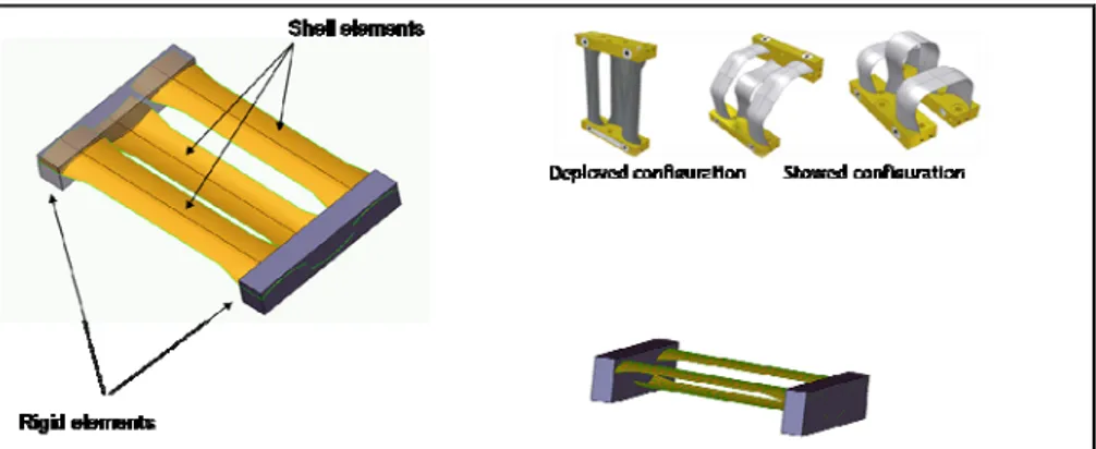
Fig. 1. 3-D modeling of the MAEVA hinge allows capturing the nonlinear phenomena responsible for generation of the elastic torque (Courtesy of AREVA and 01-METRAVIB).
A typical example is the modeling of the elastic hinges that are classically used in the design of deployable space structures. Figure 1 displays the so-called MAEVA elastic hinge. It is in fact a bistable system made of 3 elastic shells. The strain energy accumulated in the stowed configuration is sufficient to provide the torque needed to deploy the structure. The shell with opposite curvature acts as a brake at the end of the deployment. It is a typical example where 3-D elastic modeling (using geometrically nonlinear shell elements) is essential to capture the local nonlinear and buckling phenomena intervening during hinge deployment and responsible for generation of the elastic torque.
7 Superelements
Superelements can be used whenever it can be assumed that the component under consideration has linear behavior in a co-rotational frame and may thus be modeled as a linear elastic body. In which case, dynamic reduction [14] can be applied to describe it in terms of two sets of modes: a set of static modes selected for expressing the interaction with adjacent bodies and a set of vibration modes covering the dynamic behavior of the component up to an upper frequency limit. The superelement is then described in terms of two sets of parameters: displacement or force unknowns on the interface and intensities of the internal vibration modes.
The most popular dynamic reduction method is the Craig & Bampton component mode synthesis (CMS) in which the static modes result from the imposition of unit displacements on the boundary and the vibration modes are obtained in fixed boundary condition. It is the most appropriate reduction method whenever the interaction with the rest of the system results from sharing common nodes. The dual approach to CMS - referred to as McNeal dynamic reduction - consists to describe the interaction between bodies in terms of interaction forces as occurring in case of contact. In which case, the static modes are the so-called attachment modes (obtained from local application of forces), and they are complemented with eigenmodes in free-free configuration.
An interesting example of application of the superelement concept is the modeling of gear trains [9]. The current approach to model gear trains consists to express the kinematic constraints existing between gear components and try to include into the model complex effects such as teeth elasticity, backlash and friction, misalignment, etc. Most of the problems are overcome when constructing detailed, but linear finite element models of the gear components directly from their CAD geometric representation. All complex effects linked to geometry (such as misalignment) and linear elastic deformation are then automatically present in the model. Attention may then be focused on the problems of detecting in time the current contacting surfaces and adopting an appropriate contact/friction model. Contact in a gear pair is a typical example where McNeal dynamic reduction seems more appropriate than CMS.
Fig. 2. Superelement modeling of a gear pair.
Figure 2 displays an instantaneous stress distribution in a gear pair modeled by superelements and the time evolution of the contact force between teeth flanks.
8 Implicit time integration
Time integration is an essential aspect for the successful merge of multibody dynamics and finite element technology in the same context. On one hand, the presence of the high frequency spectrum
brought into the model by finite element discretization implies the adoption of an integration scheme that remains stable over the entire frequency range. On the other hand, it can be shown that the index 3 DAE equations that result from linearization of the equilibrium residual are characterized by a pair of eigenvalues at infinity for each constraint in the system. Therefore the time integration to be adopted has to be characterized by a spectral radius
ρ
< 1 over the entire frequency interval. It can be shown that, with appropriate choice of free parameters, the so-calledα
-generalized method has the remarkable property of remaining second-order accurate while offering the possibility of delivering a spectral radius 0 ≤ρ
< 1. A suitable formulation of theα
-generalized method for flexible multibody dynamics is described and its properties discussed in [12].The fast configuration changes (e.g. due to intermittent contact) that often arise in multibody systems render necessary the implementation of an adaptive time step strategy to capture high transient behavior while maintaining acceptable computational times. It is generally based on a monitoring of the local truncation error generated by the time integration algorithm [11].
Recent work also shows that it might be possible to complement the time integration algorithm with separate treatment of discontinuities in time due to contact / impact [13].
9 Co-simulation
Co-simulation can have different objectives. On the one hand, it can allow to organize communication and interaction between different softwares (e.g. multibody dynamics, finite element analysis, control) running on different processors to simulate in a concurrent manner different aspects of a same project. On the other hand, it can also be regarded as domain decomposition tool for parallel processing. Different parts of the system are then simulated in a concurrent manner by different processes with the same software [10]. Co-simulation consists then in organizing the exchange of information between processes so as to reproduce the solution in time of the complete system.
In both cases, co-simulation implies the definition of a master process that runs its own part of the model but also controls the time marching process, manages the exchange of information on the interfaces with the slave processors and verifies the convergence of the iteration process within the time step. Each slave process simulates a different part or aspect of the model and exchanges information on its own interface with the master process.
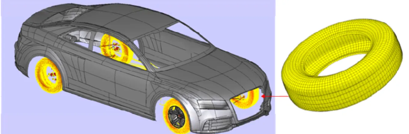
An example of co-simulation as domain decomposition tool is illustrated by Figure 3. It consists of a car model of adequate complexity to simulate standardized maneuvers for evaluating the handling and stability performances of vehicles in the higher frequency range, and to predict accurate loads for durability analysis. In this model the car body is still assumed rigid, and suspensions are defined by a mix of rigid bodies, joints and force elements, but the tires are represented by the FE model displayed on the right. Non-linear flexibility of the twist beam is considered by meshing it with shell elements.
Fig. 3 MBD car model with FE model of tires
The resulting model numbers 2.E06 DOFs. The high resolution of the FE tire model is motivated by the objective to capture the high frequency response of the suspension system to road roughness. Full details both on the co-simulation method and on the example can be found in [10]. Let us simply mention that this example has been run on a parallel machine offering variable number of processors. On the one hand, the running time for the simulation of 5 s. maneuver at 70 km/h with one single process using 6 processors has taken 70 hours of computing time. The same problem has then been split into 1 master and 5 slave processes distributed on 26 processors as follows:
− Master process: car body + wheel centers (1 processor);
− Slave process 1: twist beam (FE) + suspension models (1 processor); − Slave processes 2 to 5: 4 tire FE models (24 processors).
The computing time has been reduced by a factor of 0.23, which corresponds to linear speedup and thus maximal use of computing resources.
10 Conclusions
The purpose of this keynote presentation was to show that full integration of finite element analysis with multibody dynamics can be achieved provided that the appropriate environment for numerical simulation is put into place. Some key aspects have been briefly described in the previous sections, among which the most important ones are to use the same description of finite motion kinematics for all system components, the construction of a library of flexible elements suitable for large displacement analysis and the adoption of an implicit method of solution based upon a time integration scheme providing numerical stability over the entire frequency range. Other aspects such as the use of superelements to represent large components whenever feasible and the use of co-simulation to extend the range of current computational tools have also been discussed.
11 References
[1] Géradin M., Cardona A., Flexible Multibody Dynamics: A Finite Element Approach, John Wiley & Sons, Chichester, 2001.
[2] Bauchau O. A., Flexible Mutibody Dynamics, volume 176 of Solid Mechanics and Its Applications, Springer, 2011.
[3] Shabana, A. A. (2005). Dynamics of multibody systems. Cambridge University Press. [4] Cardona, A., & Geradin, M. (1991). Modelling of superelements in mechanism analysis.
International Journal for Numerical Methods in Engineering, 32(8), 1565-1593.
[5] Simo J., A finite strain beam formulation. The three-dimensional dynamic problem. Part I, Computer Methods in Applied Mechanics and Engineering 49 (1985) 55-70.
[6] Simo J., Fox D., On a stress resultant geometrically exact shell model. Part I: Formulation and optimal parametrization, Computer Methods in Applied Mechanics and Engineering 72 (1989) 67-304.
[7] Cardona A., Géradin M., A beam finite element non-linear theory with finite rotations, International Journal for Numerical Methods in Engineering 26 (1988) 2403-2438.
[8] Ascher U.M.; Petzold L.R. (1998) Computer Methods for Ordinary Differential Equations and Differential-Algebraic Equations. Society for Industrial and Applied Mathematics (SIAM), Philadelphia, PA.
[9] Virlez G., Brüls O., Sonneville V., Tromme E., Duysinx P, Géradin M. (2013) Contact model between superelements in dynamic multibody Systems. Paper DETC2013-13469, IDETC/CIE 2013 ASME Conference, Portland, OR.
[10] Cugnon F., Jetteur P., Pascon F., van Eekelen T. (2013) Use of an implicit non-linear FEA multi-model solver for the dynamic simulation of an automotive vehicle with meshed tires. Multibody Dynamics 2013 Conference, ECCOMAS, Zagreb, Croatia.
[11] Cardona, A., & Géradin, M. (1994). Numerical Integration of Second Order Differential— Algebraic Systems in Flexible Mechanism Dynamics. In Computer-Aided Analysis of Rigid and Flexible Mechanical Systems (pp. 501-529). Springer Netherlands.
[12] Arnold, M., & Brüls, O. (2007). Convergence of the generalized-α scheme for constrained mechanical systems. Multibody System Dynamics, 18(2), 185-202.
[13] Chen, Q.-z., Acary, V., Virlez, G. and Brüls, O. (2013), A nonsmooth generalized- α scheme for flexible multibody systems with unilateral constraints. Int. J. Numer. Meth. Engng.
[14] Géradin, M., & Rixen, D. Mechanical vibrations: theory and application to structural dynamics (third edition). John Wiley & Sons, 2014 (to appear).