A Raster SOLAP for the Visualization of Crime Data Fields
Kasprzyk Jean-Paul
e-mail: [email protected]Donnay Jean-Paul
e-mail: [email protected] University of LiegeDepartment of Geography (Geomatics Unit) Liege, Belgium
Abstract—In order to effectively extract synthetic information from large spatial data sets, Spatial OnLine Analytical Processing (SOLAP) combines Geographic Information Systems (GIS) with Business Intelligence (BI) to query data warehouses through interactive vector maps. On the other hand, crime strategical analysis is usually based on raster maps computed by Kernel Density Estimation (KDE), then independent of any artificial boundary. This paper introduces an alternative vision of SOLAP which uses the raster model (instead of the vector one) in order to integrate crime data fields computed by KDE. It allows a continuous visualization of spatial data which, until now, has not been compatible with other SOLAP tools. The original geo-model is validated by a prototype adapted to the police needs.
Keywords-Data Warehouse; Kernel Density Estimation; GIS; Business Intelligence; Crime Hotspots Analysis.
I. INTRODUCTION
In big cities like Seattle or London, crimes are prevented by allocating the available police forces in the field. In order to optimize this prevention, the identification of risk areas (crime hotspots) is based on the analysis of large amounts of
data. Indeed, in London for instance, more than one million crimes are listed each year [33].
On the one hand, GIS and BI [8] techniques include efficient tools like SOLAP to easily represent aggregated information (through tables, charts and maps) out of data warehouses [19][3]. On the other hand, police analysts usually use a KDE technique to identify crime hotspots in raster maps [12]. Indeed, these maps are efficient to visualize the distribution of crimes in a continuous space which does not depend on artificial boundaries (everyone knows the expression “crime has no boundaries”). Until now, this raster representation of data (used in crime mapping and other fields like ecology) has not been compatible with current SOLAP tools (based on the vector model).
In this paper, an original SOLAP model is suggested [18]. It considers a continuous space for the exploration of a raster data warehouse. The paper is organised as follows. In Section II, a state of the art is developed about crime mapping and SOLAP. In Section III, the raster SOLAP model is presented as well as its exploitation of KDE maps. In Section IV, the model is validated by an operational prototype including a crime data set from the Seattle police.
II. STATE OF THE ART
In this section, a state of the art about crime mapping and SOLAP is presented. A hypothesis is then drawn from this related work.
A. Crime mapping and Kernel Density Estimation
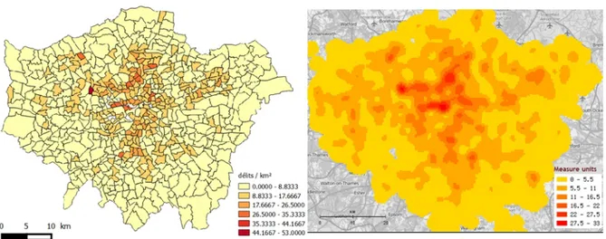
In crime mapping, crimes are basically modelled as georeferenced points [32]. However, when large clouds of points are analysed (involving thousands of data), point maps are not efficient anymore. Large data sets have to be spatially aggregated. In cartography, classical choropleth maps show data aggregations depending on pre-defined spatial entities like police sectors (Figure 1a). In this case, data are represented in a discrete space. However, hotspots identified with this method are too much influenced by the shape of artificial boundaries which are independent of analysed data (crimes). This well-known issue of geography is called the Modifiable Areal Unit Problem or MAUP [25]. To minimize MAUP, police analysts use KDE to aggregate data in a continuous space (Figure 1b). KDE generates a field where pixel values only depend on the number of crimes and their proximity in a neighbourhood area determined by a parameter called “bandwidth”. The bandwidth and the KDE function itself are the only parameters that significantly influence the field smoothing and so the shapes of the hotspots [7].
The problem with KDE is that heavy computations are needed to generate a map (especially for large data sets) and several tests are generally performed in order to determine the best parameters for the KDE function [6]. Moreover, crimes are not only characterized by space but also by other dimensions like time (for instance, months, days of the week or hours of the day) or crime type. It is thus interesting for the analyst to generate several KDE maps depending on these non-spatial dimensions (for instances, a KDE for each crime type, a KDE for each month, etc.).
B. SOLAP
An OLAP server allows decision makers to quickly query data hypercubes which are models of pre-aggregated data depending on several dimensions [9]. Users can easily navigate into data hypercubes through interactive tables (called “pivot tables”) or charts. When a data warehouse (which manages hypercubes) is spatialized, a SOLAP server can handle spatial operations through interactive maps [2]. Until now, popular SOLAP tools, like GeoMondrian [31] or Map4Decision [16], have only been able to represent spatially discrete aggregations (Figure 1a) which can be exposed to MAUP. Indeed, a classical SOLAP tool only considers vector data which are mostly efficient for spatially discrete representations. Yet in some recent researches, SOLAP models can spatially interpolate vector data on the fly [1][34] [5][35].
In GIS, the raster model is an efficient alternative to the vector one for continuous space representation [11]. This is useful for continuous phenomena analysis (temperature, precipitation, pollution, etc.) but also for continuous results of treatments applied on discrete data like KDE. In other SOLAP researches, vector grids have been considered, which are very close to the raster model [24][22][14][20][28]. The potential of raster in SOLAP, especially for continuous phenomena represented by fields, was demonstrated. Nevertheless, raster results of treatments like KDE were not considered and most of the time, validation prototypes were still implemented with the vector model (pixels stored like square polygons) whereas real raster data, stored as arrays, offer better performance for specific treatments like data aggregations on rows and columns. Moreover, data arrays are already used in Multidimensional OLAP, or MOLAP [13], which has never been considered in SOLAP. In [18], it was worked out that vector SOLAP is closer to Relational OLAP, or ROLAP [13], which uses relational database management systems like Oracle [27].
C. Hypothesis
According to SOLAP literature, an original raster SOLAP model could be developed to analyse fields resulting from KDE. Based on this model, a SOLAP prototype would allow police analysts to easily explore crime data warehouses through interactive and continuous KDE maps, but also tables and charts.
III. MODEL
In this section, OLAP basics are first explained in order to introduce our original model: raster SOLAP. Then, details are given about the way KDE fields are integrated (KDE SOLAP).
A. OLAP basics
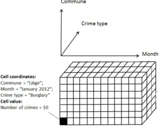
Most of OLAP models are based on multidimensional data warehouses which are conceptually described by a simple star schema [19]. An example is given in Figure 2. A dimension (branch of the star) is a finite set of members. For instance, “burglary” and “robbery” are members of the “crime type” dimension. These members can possibly be organized by a hierarchy made of children and parents belonging to different dimension levels. For instance, in the “time” dimension, “January 2012” member (belonging to the “month” level) is a child of “2012” member (belonging to the “year” level). Each possible combination of dimension members is called “fact” and a fact is always associated to a measure. For instance, “burglaries of January 2012 in Liege province” is a fact associated to a number of crimes (the measure). When it is not stored in the data warehouse, a measure (most of the time, a numerical value) is always the aggregation of fact measures belonging to a more detailed level of dimensions (more detailed facts). A
dimension can possibly be entirely aggregated. It would be the case of the “crime type” dimension if the fact was “crimes of January 2012 in Liege province” (including every crime type).
Figure 2. Example of a star schema.
An instance of a star schema is called “data hypercube” (or simply “data cube”). A cell of the cube is a fact, its value is the measure, and its coordinates in the multidimensional space are members which describe the fact. Physically, the data warehouse at least stores the “base data cube” (Figure 3). It is the cartesian product of all dimensions at the most detailed level (the set of all detailed facts). This base data cube is the minimum set of measures from which the measure of every possible fact can be computed by aggregation. In ROLAP, detailed facts are stored in a “fact table” of a relational datawarehouse. In MOLAP, detailed facts are stored in multidimensional arrays. The main advantage of ROLAP is that null facts (for which no crime is associated) do not have to be stored. In MOLAP on the other hand, even though all possible detailed facts (including unneccessary null facts) are stored, performances of aggregation operations (on rows and columns) are usually better [4][13].
Figure 3. Example of a base data cube.
Figure 4. Example of drilling and slice operations on a data cube. Typical OLAP operations are drillings and slices on dimensions. Figure 4 illustrates an example of drill down / roll up on the hierarchy of a time dimension. In this way, users can easily switch from an aggregation level of dimension to another one. The slice operations allow users to consider only one portion of the data cube. In Figure 4, the slice isolates facts linked to “Liege” member of “Province” level. By isolating a smaller data cube, slices reduce the number of aggregation operations necessary to compute the measures. On the other hand, a roll up, which shows less detailed facts, can imply heavy treatments. For this reason, in addition to the base data cube, several cuboids (data cubes at less detailed levels) can be stored in the data warehouse to speed up heavy aggregations computations [4]. Slices and drillings can be applied directly on table interfaces, charts but also maps in the case of SOLAP.
B. Raster SOLAP
In a classical SOLAP approach (vector SOLAP), data cubes handle spatialized dimensions [2][4]. Spatialized members are associated to one vector geometry (point, line or polygon) in order to represent spatialized facts on a map interface (like the one in Figure 1a). Sometimes, SOLAP involves spatialized measures which can be numeric values (distances, for instance) or geometries [15]. In this case, measures can be aggregated with spatial operations like union, intersection, etc.
In order to represent the spatial continuity, our original model considers geographical space in a very different way. Indeed, space is not a property of spatialized members anymore but it is directly included as X and Y dimensions in the star schema (Figure 5a). X and Y, simply called “spatial dimensions”, are cartographic coordinates of any point in the study area coverage [17].
Figure 5. Raster star schema and raster hypercube.
The instance of this star schema is a data hypercube where X and Y dimensions are respectively deducted from columns (C) and rows (R) of raster data (georeferenced images). It is simply called “raster hypercube” (Figure 5b). Details of the affine transformations between (X, -Y) and (C,
R) are described in [18]. In addition to X and Y, “other
dimensions” are non-spatial attributes that can be modelled in any classical OLAP environment: time, customer, product, etc.
X and Y are very particular dimensions. Spatial members
are actually pixels and they are always described by both X and Y. Like raster pyramids in GIS [26], several raster cuboids can be stored with different resolutions to represent spatial continuity at different detail levels (Figure 6). For the user, switching from a raster cube to another one is a roll up/drill down operation on spatial dimensions X, Y.
Including X and Y directly in the star schema also brings an important spatial flexibility in SOLAP. Since space is defined at the pixel level, any geographical member (Liege province, for instance) can be imported on the fly during the user’s analysis. A simple GIS operation, including a raster layer of geographical entities, identifies the space members (a set of pixels in the raster cube) which geometrically describe the new imported geographical members [18]. Then, slice and drilling operations can involve these new “geo-members” in maps, tables or charts.
Figure 6. Precomputed raster cuboids and spatial drillings.
Another original aspect of raster SOLAP comes from its physical implementation: the hybrid management of spatial and non-spatial dimensions. Indeed, spatial database management systems like PostGIS [29] or Spatial Oracle [26] allow the storage of raster arrays as attributes of relations. Therefore in our model, non-spatial dimensions can be implemented according to a classical ROLAP approach managed in SQL (ROLAP dimensions). Spatial dimensions are included in the raster attribute, considered as a measure in the ROLAP model. Aggregations of these measures are defined by map algebra [23] like in many continuous SOLAP researches: local map algebra for non-spatial aggregations and zonal map algebra for non-spatial aggregations [22][34][5][14][28]. Details of raster SOLAP operations in our model are given in [18]. Thereby, raster SOLAP inherits from advantages of ROLAP for non-spatial dimensions (null ROLAP facts do not need to be stored) but also from MOLAP advantages for raster spatial dimensions (fast spatial aggregations on rows and columns of arrays).
Let us note that by considering only the X and Y dimensions of the raster SOLAP model, a raster hypercube becomes a simple raster. As discussed in [18], there is almost no difference between a 2D MOLAP cube and a raster since they both are arrays whose coordinates refer to dimension members. In raster, the transformation from the raster space (C, R) to the geographical space (X, -Y) is always an affine transformation while other indexing techniques can be used in a MOLAP cube (depending on the modelled phenomena which can be ordered or not, continuous or discrete, etc.). As already mentioned, the raster SOLAP is implemented as a ROLAP in this research. Nevertheless, the implementation of a raster cube in a pure MOLAP environment would be an interesting perspective.
C. KDE SOLAP
The previous section introduced our original SOLAP model able to integrate raster data (raster hypercube). Since crime mapping uses KDE raster data for crime prevention, the following section presents the way KDE raster fields are integrated into a raster hypercube for SOLAP.
A KDE is a raster field where each pixel has a value depending on the number of points (like crimes) in its neighbourhood. Moreover, the distance of each neighbour point to the pixel centre also influences the KDE value. Close points have more influence than distant points.
The whole KDE raster represents a continuous surface in the geographical space (defined by X and Y). An example was given in Figure 1b. The KDE surface smoothing first depends on the KDE function itself: quartic, normal, triangular, uniform, etc. [10]. For most of KDE functions, the value of a pixel
p
j can be expressed by the following general formula:1 * ( , )
n
j i i ij
In (1), K is a KDE function (e.g., quartic),
v
i is the value of a pointi
,d
ij is the distance of a pointi
to the pixel centre j, r is a constant bandwidth and n is the number of points for whichd
ij< r. Most of the time in crime mapping,v
i
1
.When KDE is applied on a large amount of points, the treatment can be quite heavy because, for every pixel of the resulting raster,
d
ij has to be calculated for every point inside the bandwidth (a circle of radius r centred on the pixel). A raster SOLAP with KDE would imply lighter treatments during the analysis because every possible KDE raster measure (associated to a non-spatial fact) would be the result of an aggregation between pre-computed KDE raster measures (associated to detailed non-spatial facts). In this way, the number of operations to calculate a pixel value only depends on the number of detailed facts to aggregate (for instance, one fact for each month of the year). It does not depend on large amounts of points anymore. Nevertheless the total number of detailed facts in a hypercube exponentially grows with the number of dimensions [4]. For this reason, a raster hypercube cannot involve too many non-spatial dimensions to deliver rapid responses to the user.To integrate KDE fields in the raster SOLAP, the following KDE condition has to be fulfilled. Let A and B two disjoints sets of points, K(X) the raster result of a KDE function K on a set of point X:
( )
( )
(
)
K A
K B
K A B
In (2), the sum of
K A
( )
andK B
( )
is actually a local map algebra operation where the result is the sum of every homologous pixel (geometrically defined on the same geographical space). In the raster SOLAP, this formula means that the sum result of two KDE raster measures respectively associated to two facts (for instance, a fact for January and a fact for February) is the same as a KDE field computed with the points involved in both KDE facts (January and February). This condition is very important because all aggregation results given by the SOLAP have to be similar to the ones given by classical KDE computations, even if only the detailed non-spatial facts (or ROLAP facts) are pre-computed with KDE.In [18], it was demonstrated that the KDE condition is fulfilled if:
The parameters of the function K are constant: the KDE function itself (quartic, for instance) and bandwidth r.
The spatial metadata of raster fields K(A), K(B) and
( )
K A B are constant: coordinates reference
system, number of columns (C members) and rows (R members), affine transformation between raster
space (defined by C, R) and geographical space (defined by X, Y) including the raster resolution. Physically, all these parameters are defined as constraints in a metadata table of the data warehouse.
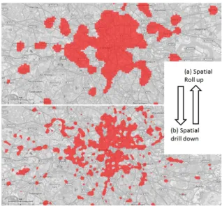
In order to adapt spatial drillings of raster SOLAP to KDE, the pre-computed raster cuboids (Figure 6) are associated to different resolutions but also to different bandwidths. For one same KDE function, bandwidth r influences the KDE surface smoothing [10][7]. In other words, the higher the KDE bandwidth is, the larger the hotspots will be. Therefore, a spatial roll up implies a more global analysis (larger hotspots) and a spatial drill down implies a more local analysis (smaller hotspots). An example is given by Figure 7 (only the first quintile of the KDE is shown to isolate hotspots).
Contrary to classical SOLAP tools where the spatial drilling is defined by semantic levels (e.g., street level, commune level, province level, etc.), this alternative spatial drilling, defined by resolution/bandwidth, is not influenced by artificial boundaries. However, the choice of the bandwidth in a KDE leads to another MAUP issue as it significantly changes the shape of the hotspots. As already mentioned in Section IIa, in classical KDE, the police analysts empirically determine an optimal bandwidth using several tests (computations with different bandwidth values). With KDE SOLAP, analysts can easily and quickly test the bandwidth values by simply drilling space (until they find the best scale analysis amongst the pre-computed cuboids). In the case study of the following section, four drillings levels are arbitrary determined in order to fit to the user’s needs and to the extent of the study area. A detailed methodology for the determination of these scale levels could be the subject of a future research about KDE SOLAP.
Figure 7. Spatial drilling on KDE SOLAP. (2)
IV. VALIDATION
In this section, a case study about Seattle crime data is first introduced. Then, our research is validated by a raster SOLAP prototype (Raster Cube) which integrates Seattle crime fields.
A. Case study
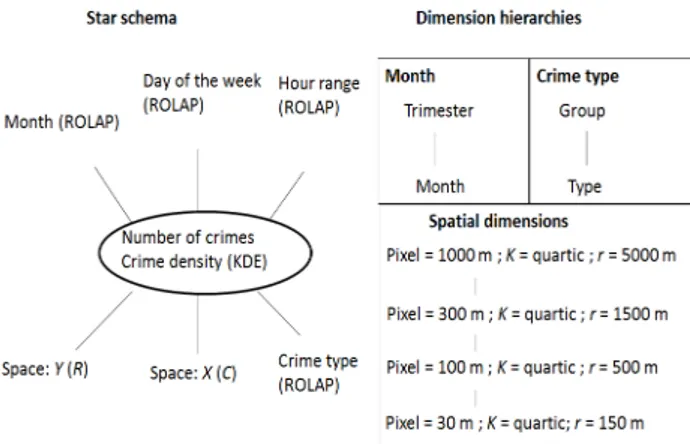
The SOLAP raster model is validated by a prototype including several data sets. Amongst them, a raster hypercube is built with Seattle crime data. These data come from 911 calls received during the year 2013 [30]. They represent around 800 000 crimes. The star schema and the description of dimension hierarchies are shown in Figure 8. Four non-spatial dimensions are modelled as ROLAP in a PostGIS data warehouse: three time dimensions (month, day of the week and range of three hours) and a crime type dimension. According to the number of detailed members for the four non-spatial dimensions, the theoretical number of detailed non-spatial facts is equal to the following: 12 (month) * 7 (day of the week) * 8 (hour range) * 25 (crime type) = 16 800. Actually, the ROLAP management of these dimensions allowed to store only 11 304 facts because 33% of the theoretical detailed facts were null (no crime).
The two spatial dimensions (X, Y) are included in the raster measures of the data warehouse. These raster measures have two distinct values: the number of crimes (used for tables and charts) and the crime density resulting from KDE (used for maps). The spatial dimensions have four pre-computed levels depending on raster resolution (30 m for the base cube, 100 m, 300 m and 1000 m for the different cuboids). As advised by [6], a quartic KDE function was used with a bandwidth r equal to the raster resolution multiplied by 5. The users can then drill the spatial dimensions until they find the best scale for their analysis.
Figure 8. Star schema and dimension hierarchies for Seattle crime data.
B. Raster Cube prototype
The prototype, called “Raster Cube”, is based on a web architecture. On the server side, the SOLAP, written in php, interrogates the PostGIS data warehouse and delivers results to the client side in HTML/Javascript. MapServer [21] was also used as a spatial data server. Raster Cube is accessible for demonstration at the following URL: http://nolap01.ulg.ac.be/rastercube .
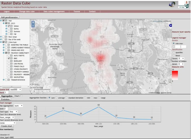
Figure 9 is a screenshot of the user interface. The dimension tree on the left shows non-spatial dimension members organized by hierarchies. The users can check all the members they choose to slice the raster hypercube before its aggregation. For instance, the slices defined in Figure 9 implies the aggregation of all crimes of the “bike” type that happened in the “winter” trimester for the whole study area (Seattle). When the “aggregation” button is pressed, “crime density” measures (KDE) are shown on the map and “number of crimes” measures are shown on charts. The map always shows the two spatial dimensions (X, Y) and charts show non-spatial dimensions. In Figure 9, one non-spatial dimension is shown by the chart: the hour range. With an additional dimension, the interface could also show, for instance, one “hour range” chart for each day of the week (still with the slices on “winter” and “bike”).
As already mentioned, in addition to the continuous map representation, raster SOLAP is also able to import new geographical members on the fly. Indeed, the users can interactively digitize spatial entities like police sectors and so add them to the dimension tree. These new “geo-members” can then be involved in spatial slices (to reduce the study area) or they can be considered as a dimension shown in charts. For instance, the evolution of “bike” crimes in the day could be easily compared with a chart for each police sectors imported on the fly.
As shown in Figure 7, space can be drilled by choosing the right cuboid and so the KDE map can be adjusted to the best analysis scale. It is also possible to generate an evolution map that for instance shows the density difference between trimesters “winter” and “spring”. This is very useful to quickly see where criminality increased and where it decreased. A few options also allow users to change the classification method of the map (linear, quantiles, etc.). Finally, a module was made to automatically build the raster hypercube from a vector data warehouse (where crimes are geometrically defined as points) and from an XML file defining the star schema. This includes the KDE computation of all non-spatial detailed facts that have to be stored in the raster data warehouse. Indeed, it is worth recalling that even if maps resulting from KDE SOLAP are identic to the one resulting from classical KDE, the way KDE are computed during the analysis is very different in this research. In a classical KDE, the field computation is based on a cloud of point (1). In KDE SOLAP, the field computation is an aggregation of pre-computed KDE raster fields which are stored in the data warehouse.
Figure 9. Raster cube interface with Seattle crime data. V. CONCLUSION AND FUTURE WORK
The aim of this paper was the presentation of a raster SOLAP model adapted to the needs of the police for the exploration of large crime data sets. A quick state of the art about crime mapping showed that police analysts generally use a KDE raster technique to represent crimes in continuous maps. At the same time, a state of the art about SOLAP showed that current tools are vector and so not compatible with KDE raster maps (despite a few researches that demonstrated the potential of raster SOLAP data cubes).
After a brief description of the main OLAP concepts (multidimensional analysis, star schema, data hypercube, drillings and slices operations), an original raster SOLAP model [18] was introduced. Opposite to vector SOLAP tools (where space is modelled with geometries associated to semantic dimension members), raster SOLAP directly includes space inside the star schema (X and Y dimensions). It offers two main advantages. First, the SOLAP can generate continuous raster maps resulting from classical drilling and slice operations (on space or other dimensions).
Then, geographical members can easily be imported on the fly during the user’s analysis.
By adapting the raster SOLAP model to KDE, the tool became able to generate continuous KDE maps like the ones usually computed by police analysts. For the police, it offers an intuitive interface to explore data warehouses, including tables, charts and continuous KDE maps. Therefore, any combination of dimension members (through OLAP operations) leads to a KDE map which is usually computed case by case by crime analysts. Moreover, drillings and slices on space respectively allow the interactive adjustment of the scale and the study area shown by the map. All these concepts were validated by an operational prototype integrating crime data from Seattle.
In conclusion, this paper explained an alternative way to integrate space in an OLAP. Compared to vector, raster SOLAP can be useful for any domain which implies a continuous representation of space (fields): crime mapping, but also ecology, agriculture, epidemiology, climatology, etc. Moreover, when a SOLAP involves fields like KDE, it suffers less from the influence of artificial boundaries (MAUP) which can bias the analysis done with a traditional
vector SOLAP. Nevertheless, raster and vector can be seen as two complementary approaches. Raster SOLAP, close to MOLAP, can handle dense data hypercubes described by few dimensions (global approach) and vector SOLAP, close to ROLAP, can handle less dense data hypercubes characterized by more dimensions (detailed approach). A hybrid (raster/vector) SOLAP, an interesting perspective of this research, could be a powerful tool allowing an efficient analysis of every type of spatial phenomena (discrete or continuous).
REFERENCES
[1] T. O. Ahmed and M. Miquel, “Multidimensional structures dedicated to continuous spatiotemporal phenomena”, Proceedings of the Twenty-Second British National Conference on Databases: Enterprise, skills and innovation, Sunderland : Springer-Verlag, 2005, pp. 29-40.
[2] Y. Bédard, “Spatial OLAP”, Forum annuel sur la R-D, Géomatique VI: Un monde accessible, Montréal, November 1997.
[3] Y. Bédard, “Beyond GIS: Spatial Online Analytical Processing and Big Data”, The 2014 Dangermond Lecture, Santa-Barbara, 2014.
[4] S. Bimonte, Integration of geographic information in data warehouses and online analysis: from modeling to visualization (Intégration de l’information géographique dans les entrepôts de données et l’analyse en ligne: de la modélisation à la visualisation), PhD, Institut National des Sciences Appliquées de Lyon, Lyon, 2007.
[5] S. Bimonte and M. A. Kang, “Towards a model for the multidimensional analysis of field data, in Proceedings of the Fourteenth east European conference on advances in databases and information systems”, B. Catania, M. Ivanovic and B. Thalheim, Eds. Berlin : Springer-Verlag, 2010, pp. 58-72.
[6] S. P. Chainey, L. Tompson and S. Uhlig, “The utility of hotspot mapping for predicting spatial patterns of crime”, Security Journal, vol. 21, 2008, pp. 4-28.
[7] S. Chainey, “Examining the influence of cell size and bandwidth size on kernel density estimation crime hotspot maps for predicting spatial patterns of crime”, Bulletin of the Geographical Society of Liege, vol. 60, 2013, pp. 7-19.
[8] T. Chee, L. K. Chan, M. H. Chuah, C. S. Tan, S. F. Wong and W. Yeoh, “Business Intelligence systems: state-of-the-art review and contemporary applications, Symposium on Progress in Information and Communication Technology”, Kuala Lumpur, 2009.
[9] E. F. Codd, S. B Codd and C. T. Salley, Providing OLAP (On-line Analytical Processing) to User-Analysts: An IT Mandate, E.F Codd and Associates, 1993.
[10] M. Di Salvo, M. Gadais and G. Roche-Woillez, The kernel density estimation : methods and tools (L’estimation de la densité par la méthode du noyau: méthodes et outils), Lyon : Certu, 2005.
[11] J. P. Donnay, “Formalization of geographic information in raster”. Revue internationale de géomatique, vol. 15, no. 4, 2005, pp. 415-438.
[12] J. E. Eck, S. P. Chainey, J. G. Cameron, M. Leitner and R. E. Wilson, “Mapping crime: Understanding hot spots”, Washington: National Institute of Justice, 2005.
[13] B. Espinasse, Data warehouses: OLAP systems: ROLAP, MOLAP and HOLAP (Entrepôt de données: Systèmes OLAP: ROLAP, MOLAP et HOLAP). Ecole Polytechnique Universitaire de Marseille, 2013.
[14] L. I. Gomez, S. A. Gomez and A. Vaisman, “A generic data model and query language for spatiotemporal OLAP cube analysis”. Proceedings of the Fifteenth International Conference on Extending Database Technology, Berlin : ACM, 2012, pp. 300-311.
[15] J. Han, N. Stefanovic and K. Koperski, “Selective materialization: an efficient method for spatial data cube construction”, Proceedings of the Second Pacific-Asia Conference on Knowledge Discovery and Data Mining, Melbourne : Springer-Verlag, 1998, pp. 144-158.
[16] Intelli³, available at <http://www.intelli3.com>, [retrieved : march, 2016].
[17] ISO 19123. Geographic information - Schema for coverage geometry and functions, 2005.
[18] J. P. Kasprzyk, Integration of spatial continuity in the multi-dimensional structure of a data warehouse – raster SOLAP (Intégration de la continuité spatiale dans la structure multidimensionnelle d’un entrepôt de données – SOLAP raster). PhD. Université de Liège, 2015, Available at <http://hdl.handle.net/2268/182360>.
[19] R. Kimball and M. Ross, The Data Warehouse Toolkit: The Definitive Guide to Dimensional Modeling, Third Edition, New York : John Wiley and Sons, 2013.
[20] J. Li, L. Meng, F. Z. Wang, W. Zhang and W. Cai. “A Map-Reduce-enabled SOLAP cube for large-scale remotely sensed data aggregation”, Computers and Geosciences, vol. 70, 2014, pp. 110-119.
[21] Mapserver 7.0.0 beta1 documentation, available at <http://mapserver.org/>, [retrieved: march, 2016].
[22] R. McHugh, Integration of the matrix structure in spatial cubes (Intégration de la structure matricielle dans les cubes spatiaux), Master thesis. Université Laval, Québec, 2008.
[23] J, Mennis, R. Viger and C. D. Tomlin, “Cubic Map Algebra functions for spatio-temporal analysis, Cartography and Geographic Information Systems”, vol. 30, no. 1, 2005, pp. 17–30.
[24] M. Miquel, Y. Bédard and A. Brisebois, “Conception of geospatial data warehouses from heterogeneous sources: application example in forestry” (Conception d’entrepôts de données géospatiales à partir de sources hétérogènes : Exemple d’application en foresterie), Ingénierie des Systèmes d’Information, vol. 7, no. 3, 2002, pp. 89-111.
[25] S. Openshaw, The modifiable areal unit problem. Norwick (Norfolk), Geo Books, 1983.
[26] Oracle, Georaster overview and concepts, available at <https://docs.oracle.com/html/B10827_01/geor_intro.htm>, [retrieved: march, 2016].
[27] Oracle, Business intelligence, available at
<http://www.oracle.com/us/solutions/business-analytics/businessintelligence/overview/index.htm>, [retrieved : march, 2016].
[28] M. Plante, Towards matrix cubes supporting on the fly spatial analysis in decision support (Vers des cubes matriciels supportant l’analyse spatiale à la volée dans un contexte décisionnel), Master thesis, Université Laval, Québec, 2014.
[29] P. Racine, and S. Cumming, Store, manipulate and analyze raster data within the PostgreSQL/PostGIS spatial database. FOSS4G, Denver, September 2011.
[30] Seattle Police, Seattle Open data, available at <https://data.seattle.gov/>, [retrieved: march, 2016].
[31] Spatialytics, Open Source GeoBI, available at <http://www.spatialytics.org/>, [retrieved: march, 2016].
[32] M. Trotta, C. Deprez and J. P. Donnay, “Impact of the environmental anisotropy in geographic profiling studies”, SAGEO 2014, Grenoble, october 2014.
[33] UK Police, Crime Map, available at <http://www.police.uk>, [retrieved: march, 2016].
[34] A. Vaisman and E. Zimanyi, “A multidimensional model representing continuous fields in spatial data warehouses”, Proceedings of the 17th ACM SIGSPATIAL International
Conference on Advances in Geographic Information Systems, Seattle : ACM, 2009, pp. 169-177.
[35] M. Zaamoune, S. Bimonte, F. Pinet and P. Beaune, “Integration of incomplete continuous data fields in OLAP: from conceptual modeling to implementation” (Intégration des données champs continus incomplets dans l’OLAP : de la modélisation conceptuelle à l’implémentation), 9e journées francophones sur les Entrepôts de Données et l'Analyse en ligne, Blois, 2013.