A Hybrid Spline Metamodel for Photovoltaic/Wind/Battery Energy Systems

O

pen

A

rchive

T

OULOUSE

A

rchive

O

uverte (

OATAO

)

OATAO is an open access repository that collects the work of Toulouse researchers and

makes it freely available over the web where possible.

This is an author-deposited version published in :

http://oatao.univ-toulouse.fr/

Eprints ID : 13773

To cite this version

_{: Zaibi, Malek and Layadi, Toufik Madani and}

Champenois, Gérard and Roboam, Xavier and Sareni, Bruno and

Belhadj, Jamel A Hybrid Spline Metamodel for

Photovoltaic/Wind/Battery Energy Systems. (2015) In: 6th

International Renewable Energy Congress - IREC 2015, 24 March

2015 - 26 March 2015 (Sousse, Tunisia)

Any correspondance concerning this service should be sent to the repository

administrator:

staff-oatao@listes-diff.inp-toulouse.fr

A Hybrid Spline Metamodel for

Photovoltaic/Wind/Battery Energy Systems

Malek Zaibi

, Toufik Madani Layadi

, G´erard Champenois

, Xavier Roboam

, Bruno Sareni

and Jamel Belhadj

1_{Universit´e de Tunis El Manar, LSE-ENIT, BP 37, 1002 Tunis Le Belv´ed`ere, Tunisia}

Email: malek.zaibi@univ-poitiers.fr – Jamel.Belhadj@esstt.rnu.tn

2_{Universit´e de Poitiers, LIAS-ENSIP, B25, TSA 41105 86073 Poitiers cedex 9, France}

Email: gerard.champenois@univ-poitiers.fr

3_{Universit´e Ferhat Abbas S´etif, S´etif 1, LAS, S´etif, Algeria}

Email: layaditm@gmail.com

4_{Universit´e de Toulouse, LAPLACE-ENSEEIHT, 2 Rue Camichel 31071 Toulouse Cedex, France}

Email: xavier.roboam@laplace.univ-tlse.fr – bruno.sareni@laplace.univ-tlse.fr

Abstract—This paper proposes a metamodel design for a

Photovoltaic/Wind/Battery Energy System. The modeling of a hybrid PV/wind generator coupled with two kinds of storage i.e. electric (battery) and hydraulic (tanks) devices is investigated. A metamodel is carried out by hybrid spline interpolation to solve the relationships between several design variables i.e. the design parameters of different subsystems and their associate response variables i.e. system indicators performance. The developed model has been successfully validated under real test conditions.

Keywords—Hybrid power systems, Metamodeling, Battery man-agement systems, Hydraulic systems.

I. INTRODUCTION

For complex systems like renewable energy sources, the design assigns highly computation-intensive process for analy-ses and simulations. Multiple techniques in engineering design and other disciplines have been developed to reduce the computational burden of evaluating numerous designs. Re-searchers have employed several metamodeling techniques in design and optimization, among which a simpler approximate model named “metamodel” can replace the original system process [1]. For example, the latter makes use of polynominal functions to solve the relationships between several design variables and one or more response variables. Many authors have suggested various types of metamodels among others: classical polynominal function models [2], stochastic models such as the Kriging interpolation model [3],[4],[5] and artificial neural network models [6], [7]. The aim of the present paper is to introduce another metamodel named as hybrid spline model. Due to the complexity of system (approximation model, design variable and problem formulation) the hybrid spline model will be developed. Hence, we use the metamodel to solve the optimization problem. This paper contains three major parts. First, the hybrid Photovoltaic (PV)/Wind Turbines (WT) sources with battery bank powering electrical and hydraulic loads is presented. Second, the metamodel-based global system process is carried out. The metamodel process is based on three steps: Design space sampling of the real-model, param-eter extraction of the metamodel and metamodel validation. Finally, the metamodel is used for assessing the hybrid system

performance.

II. SYSTEM DESCRIPTION

The present system includes hybrid Photovoltaic (PV)/Wind turbines (WT) sources with battery bank powering electrical loads and hydraulic network loads. The latter is composed of water pumping and Reverse Osmosis (RO) desalination unit to produce permeate water. Fig.1 presents the global system architecture. The PV/WT/Battery system consists of photovoltaic panels, wind turbines, battery bank and converters (DC/DC and AC/DC). The brackish water pumping and desalination process are composed of two motor-pumps, RO membrane, two water tanks and two (DC/AC) inverters. The different subsystems are coupled to DC Bus. The meteorological profiles: wind speed (𝑉𝑤𝑖𝑛𝑑),

solar irradiation (𝐼𝑟) and ambient temperature (𝑇𝑎) of a

typical region (North Tunisia) have been recorded for one year.

A. Hybrid Energy Models

1) PV generator model: The PV generator power is deter-mined from a model as defined in [8]-[9]:

𝑃𝑃 𝑉 = 𝜂𝑟⋅ 𝜂𝑝𝑐⋅ [1 − 𝛽 ⋅ (𝑇𝑐− 𝑁 𝑂𝐶𝑇 )] ⋅ 𝐴𝑃 𝑉 ⋅ 𝐼𝑟 (1)

where 𝜂𝑟 is PV efficiency, 𝜂𝑝𝑐 the power tracking

equip-ment efficiency, which is equal to 0.9 with a perfect maximum point tracker, 𝛽 the temperature coefficient, ranging from 0.004 to 0.006 per∘_{C for silicon cells, 𝑁 𝑂𝐶𝑇 normal operating PV}

cell temperature (∘_{C), 𝐴}

𝑃 𝑉 the PV panels area (m2) and 𝑇𝑐

the PV cell temperature (∘_{C) which can be expressed by [10]:}

𝑇𝑐 = 30 + 0.0175 ⋅ (𝐼𝑟− 300) + 1.14 ⋅ (𝑇𝑎− 25) (2)

where 𝑇𝑎 denotes the ambient temperature (∘C).

Fig. 1. Global system architecture

2) Wind turbine model: The wind turbine power is ex-pressed as follows [11]: 𝑃𝑤𝑡= 1 2⋅ 𝐶𝑝⋅ 𝜌 ⋅ 𝐴𝑤𝑡⋅ 𝑉 3 𝑤𝑖𝑛𝑑 (3)

where 𝐶𝑝 is the wind turbine power coefficient, 𝜌 the air

mass density and 𝐴𝑤𝑡 the wind turbine swept area.

3) Battery storage model: In this study, we propose an ideal model for the battery. During the charging and discharg-ing process, the state of charge (𝑆𝑂𝐶) vs time (𝑡) can be described by [12]: 𝑆𝑂𝐶(𝑡) = { 𝑆𝑂𝐶(𝑡 − Δ𝑡)+ 𝜂𝑐ℎ⋅𝑃𝐵𝑎𝑡_𝐶𝐵𝑎𝑡/𝑈𝑏𝑢𝑠 𝑛 ⋅ Δ𝑡 𝑆𝑂𝐶(𝑡 − Δ𝑡)+ 1 𝜂𝑑𝑖𝑠⋅ 𝑃𝐵𝑎𝑡/𝑈𝑏𝑢𝑠 𝐶𝐵𝑎𝑡 𝑛 ⋅ Δ𝑡 } (4) where Δ𝑡 is the time step (here, three minutes), 𝑃𝐵𝑎𝑡

represents the battery power, 𝜂𝑐ℎ and 𝜂𝑑𝑖𝑠 are respectively the

battery efficiencies during charging and discharging phases. 𝑈𝑏𝑢𝑠denotes the nominal DC bus voltage. 𝐶𝑛𝐵𝑎𝑡represents the

nominal capacity of the battery bank in Ampere hour (Ah). At any time step Δ𝑡, the 𝑆𝑂𝐶 must comply with the following constraints:

𝑆𝑂𝐶𝑚𝑖𝑛≤ 𝑆𝑂𝐶(𝑡) ≤ 𝑆𝑂𝐶𝑚𝑎𝑥 (5)

where 𝑆𝑂𝐶𝑚𝑖𝑛 and 𝑆𝑂𝐶𝑚𝑎𝑥are the minimum and

max-imum allowable storage capacities, respectively.

4) Electrical load profile: Typical power consumption (𝑃𝑙𝑜𝑎𝑑) data were acquired for a residential home. During

365 days with three minutes acquisition period, this profile describes the weekdays and weekend days consumption (see Fig.2).

B. Hydraulic network models

The hydraulic network is shown in Fig.1. It includes four principal subsystems: the motor-pump 1 which draws water from well, a water storage tank 1, the high pressure motor-pump 2 associated with a reverse osmosis desalination device and a water tank storage 2. this final storage is placed at the output of the desalination process to store fresh water.

1) Model of the motor-pump 1: The GRUNDFOS⃝R

motor-pump (“CRN” type) was selected for motor-pumping water from well to the tank water storage 1. The electric power 𝑃1required for

motor-pump 1 at head H and flow rate 𝑄1 can be calculated

as [13]:

𝑃1=

𝜌𝑤⋅ 𝑔 ⋅ 𝐻 ⋅ 𝑄1

𝜂𝑚⋅ 𝜂𝑝

(6)

where 𝜌𝑤 is the density of water (kg/m3), g the gravity

constant (m/s2_{), 𝜂}

𝑚 the motor efficiency and 𝜂𝑝 the pump

Fig. 2. Weekly power consumption profile

2) Model of the water storage tank 1: Water tank 1 is used to store brackish water. It is characterized by its water level 𝐿1

and its section 𝑆1. The level 𝐿1 can be calculated as follows:

𝐿1(𝑡) = 𝐿1(𝑡 − Δ𝑡) +

(𝑄1(𝑡) − 𝑄2(𝑡))

𝑆1

⋅ Δ𝑡 (7) This tank is fitted with four sensors measuring four differ-ent water levels: two minimum sublevels, i.e. high and low (𝐿1

𝑚𝑖𝑛𝐻 and 𝐿 1

𝑚𝑖𝑛𝐿) and two maximum sublevels, i.e high

and low (𝐿1

𝑚𝑎𝑥𝐻 and 𝐿1𝑚𝑎𝑥𝐿). The high and low levels are

separated by a hysteresis band. This hysteresis avoids the switch On/Off of the motor-pump during operation.

3) Model of the motor-pump 2 with reverse osmosis membrane: The GRUNDFOS⃝R _{motor-pump (“CRN” type)}

[13] was selected for water pumping from the tank water storage 1 to the tank water storage 2 via a reverse osmosis (RO) desalination system (ROMEMBRA⃝R _{TORAY RO}

membrane, “TM” type [14]). In this study, the RO membrane model is characterized by the nominal fresh (permeate) water production in day 𝐷𝑀 (m3_/d).

Three design configuration between the motor-pumps and RO membrane are used to develop a model (from a fitting approach). Fig.3 presents three RO membrane characteristics 𝐻2(𝑄2) and the Fig.4 shows three motor-pump characteristics

𝑃2(𝑄2) with their efficiencies.

The expression of the flow rate 𝑄2 is a function of the

electric power 𝑃2 and the nominal fresh water 𝐷𝑀 :

𝑄2= 4.77 ⋅ 10−6⋅ 𝑃20.54⋅ 𝐷𝑀2.843+ 0.025 ⋅ 𝑃20.578 (8)

Moreover, the expression of the minimal and maximal electri-cal powers, respectively 𝑃2𝑚𝑖𝑛 and 𝑃2𝑚𝑎𝑥 is a function of the

nominal fresh water 𝐷𝑀 : { 𝑃𝑚𝑖𝑛 2 = 53.64 ⋅ 𝐷𝑀0.63 𝑃𝑚𝑎𝑥 2 = 384 ⋅ 𝐷𝑀0.93 (9)

Fig. 3. Different RO membrane characteristics

Fig. 4. Different motor-pump characteristics

For the RO process, the flow rate 𝑄2is separated between

the permeate flow 𝑄2𝑎 and the concentrate flow 𝑄2𝑏.

{

𝑄2𝑎= 𝑇𝑐⋅ 𝑄2

𝑄2𝑏= 𝑄2− 𝑄2𝑎 (10)

where 𝑇𝑐 is the conversion rate of the RO membrane (i.e.

𝑇𝑐=20%).

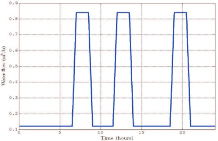
4) Modeling of the fresh water storage tank 2: Water storage tank 2 is the tank of the permeate (fresh) water. It is characterized by the level 𝐿2 and section 𝑆2. The level 𝐿2

can be calculated as follows:

𝐿2(𝑡) = 𝐿2(𝑡 − Δ𝑡) +

(𝑄2𝑎(𝑡) − 𝑄𝑙𝑜𝑎𝑑(𝑡))

𝑆2

⋅ Δ𝑡 (11) where 𝑄𝑙𝑜𝑎𝑑 is the water flow demand required by the

consumers. Fig.5 represents the daily water flow demand. As previously, this tank is fitted with four level sensors: two useful levels, i.e. high and low (𝐿2

𝑢𝐻 and 𝐿2𝑢𝐿) and two

maximum levels, i.e. high and low (𝐿2

𝑚𝑎𝑥𝐻 and 𝐿 2

𝑚𝑎𝑥𝐿). The

Fig. 5. Daily water flow profile

C. System indicators performance

To assess the performance of this complex system, three indicators are used as follows:

1) The Loss of electric Power Supply Probability (𝐿𝑃 𝑆𝑃𝐸), 𝐿𝑃 𝑆𝑃𝐸(%) = 𝑇 ∑ Δ𝑡=1 Δ𝑃 (Δ𝑡) ⋅ Δ𝑡 𝑇 ∑ Δ𝑡=1 𝑃𝑙𝑜𝑎𝑑(Δ𝑡) ⋅ Δ𝑡 (12) with Δ𝑃 = { 𝑃𝑙𝑜𝑎𝑑− 𝑃𝑟𝑒, 𝑆𝑂𝐶≤ 𝑆𝑂𝐶𝑚𝑖𝑛 0, 𝑜𝑡ℎ𝑒𝑟𝑤𝑖𝑠𝑒 (13)

where 𝑃𝑟𝑒 is the renewable source power and 𝑃𝑙𝑜𝑎𝑑

is the electrical load power.

2) The Loss of hydraulic Power Supply Probability (𝐿𝑃 𝑆𝑃𝐻), 𝐿𝑃 𝑆𝑃𝐻(%) = 𝑇 ∑ Δ𝑡=1 𝑄(Δ𝑡) ⋅ Δ𝑡 𝑄𝑙𝑜𝑎𝑑⋅ 𝑇 (14) where 𝑄= { 𝑄𝑙𝑜𝑎𝑑, 𝐿2= 0 0, 𝑜𝑡ℎ𝑒𝑟𝑤𝑖𝑠𝑒 (15)

3) The exchange energy by the battery (𝐸𝑒𝑥𝑐ℎ𝑎𝑛𝑔𝑒)

𝐸𝑒𝑥𝑐ℎ𝑎𝑛𝑔𝑒(𝑘𝑊 ℎ) = 𝑇

∫

0

∣𝑃𝐵𝑎𝑡∣ ⋅ 𝑑𝑡 (16)

To obtain the performance of the three system indica-tors, a dynamic simulator is developed using MATLAB⃝R

environment[12]. The different models of the studied system are integrated in the dynamic simulator. The latter during one year with sample time of three minutes allows us to simulate the system evolution.

III. METAMODEL-BASED PROCESS

The proposed metamodel process is summarized in Fig.6. The first step resides in the sampling of the design space with the dynamic simulator. Then the building of the metamodel is performed to deduce the predicted responses. finally the validation step of the metamodel is presented.

A. Design Space Sampling

The relationships between the design variables and the system indicators performance characterized from the dynamic simulator. Given a set of 𝑚 design sites 𝑆 = [𝑠1. . . 𝑠𝑚]𝑇

with 𝑠𝑖∈ ℜ𝑛 (n: numbers of design variables) and responses

𝑌 = [𝑦1. . . 𝑦𝑚]𝑇 with 𝑦𝑖∈ ℜ𝑝(p: numbers of responses). For

the design site 𝑠𝑖, the design variables is,

𝑠𝑖=

[

𝐴𝑝𝑣, 𝐴𝑤𝑡, 𝐶𝑛𝐵𝑎𝑡, 𝑆𝑂𝐶𝑢, 𝐿2𝑢, 𝑆2, 𝑃1, 𝐷𝑀

]

𝑖 (17)

The responses 𝑦𝑖versus the system indicators performance are,

𝑦𝑖 = [𝐿𝑃 𝑆𝑃𝐸, 𝐿𝑃 𝑆𝑃𝐻, 𝐸𝑒𝑥𝑐ℎ𝑎𝑛𝑔𝑒]_𝑖 (18)

The space filling design, the sample points around the border and only put few points in the interior of the design space:

𝑆= ⎛ ⎜ ⎜ ⎜ ⎜ ⎜ ⎜ ⎜ ⎜ ⎜ ⎜ ⎜ ⎜ ⎜ ⎜ ⎝ 𝐴𝑝𝑣: 𝑥1= {𝑥𝑚𝑖𝑛1 , 𝑥𝑚𝑖𝑛 1 +𝑥 𝑚𝑎𝑥 1 2 , 𝑥 𝑚𝑎𝑥 1 } 𝐴𝑤𝑡: 𝑥2= {𝑥𝑚𝑖𝑛2 , 𝑥𝑚𝑖𝑛 2 +𝑥𝑚𝑎𝑥2 2 , 𝑥 𝑚𝑎𝑥 2 } 𝐶𝑛𝐵𝑎𝑡: 𝑥3= {𝑥𝑚𝑖𝑛3 , 𝑥𝑚𝑖𝑛 3 +𝑥 𝑚𝑎𝑥 3 2 , 𝑥 𝑚𝑎𝑥 3 } 𝑆𝑂𝐶𝑢: 𝑥4= {𝑥𝑚𝑖𝑛4 , 𝑥𝑚𝑖𝑛 4 +𝑥 𝑚𝑎𝑥 4 2 , 𝑥 𝑚𝑎𝑥 4 } 𝐿2 𝑢: 𝑥5= {𝑥𝑚𝑖𝑛5 , 𝑥𝑚𝑖𝑛 5 +𝑥 𝑚𝑎𝑥 5 2 , 𝑥 𝑚𝑎𝑥 5 } 𝑆2: 𝑥6= {𝑥𝑚𝑖𝑛6 , 𝑥𝑚𝑖𝑛 6 +𝑥𝑚𝑎𝑥6 2 , 𝑥 𝑚𝑎𝑥 6 } 𝑃1: 𝑥7= {𝑥𝑚𝑖𝑛7 , 𝑥𝑚𝑖𝑛 7 +𝑥 𝑚𝑎𝑥 7 2 , 𝑥 𝑚𝑎𝑥 7 } 𝐷𝑀 : 𝑥8= {𝑥𝑚𝑖𝑛8 , 𝑥𝑚𝑖𝑛 8 +𝑥 𝑚𝑎𝑥 8 2 , 𝑥 𝑚𝑎𝑥 8 } ⎞ ⎟ ⎟ ⎟ ⎟ ⎟ ⎟ ⎟ ⎟ ⎟ ⎟ ⎟ ⎟ ⎟ ⎟ ⎠ (19)

B. Parameter extraction of the Metamodel

The design space data were used for the model fitting to ex-plore the best polynomial function. Those data were employed using MATLAB⃝R _{Model-Based Calibration Toolbox. In this}

toolbox, two main global linear models are developed such as polynomial or hybrid splines. After testing these models, the hybrid splines models are used to predict the system indicators performance. The hybrid spline model is a piecewise polynomial function, where different sections of polynomial are fitted smoothly together. The locations of the breaks are called knots. The required number of knots (up to a maximum of 50) and their positions are chosen. In this case all the pieces of curves between the knots are formed from polynomial of the same order (the order up to 3).

C. Metamodel validation

The predicted responses obtained from the hybrid spline model were compared with simulator dynamic responses for testing and validating the metamodel. Different points are used to validate the metamodel. There are two measures of the accurate model, defined as below:

∙ The Root Mean Square Error (𝑅𝑀 𝑆𝐸) is:

𝑅𝑀 𝑆𝐸= v u u u ⎷ 𝑁 ∑ 𝑖=1 (𝑦𝑖− ˆ𝑦𝑖)2 𝑁 (20)

Fig. 6. Metamodel design process

∙ The 𝑅 square value, coefficient of determination, (𝑅2₎

is: 𝑅2= 1 − 𝑁 ∑ 𝑖=1 (𝑦𝑖− ˆ𝑦𝑖)2 𝑁 ∑ 𝑖=1 (𝑦𝑖− 𝑦)2 (21)

where 𝑁 is the number of validation points;𝑦_ˆ𝑖is the predicted

value for the observed value 𝑦𝑖; 𝑦 is the mean of the observed

values at the validation points.

IV. RESULTS AND DISCUSSION

Following the proposed process, the constraints of the design variables are defined as

⎧          ⎨          ⎩ 30 m2_{≤ 𝐴} 𝑝𝑣 ≤ 90 m2 60 m2_{≤ 𝐴} 𝑤𝑡≤ 220 m2 400 Ah ≤ 𝐶𝐵𝑎𝑡 𝑛 ≤ 600 Ah 30 % ≤ 𝑆𝑂𝐶𝑢≤ 100 % 0.3 m ≤ 𝐿2 𝑢≤ 1.9 m 2 m2_{≤ 𝑆} 2≤ 20 m2 600 W ≤ 𝑃1≤ 1600 W 7 m3_{/d≤ 𝐷𝑀 ≤ 30 m}3_/d (22)

For each design variable, three values (minimal, mean and maximal) are used to obtain the following design space 𝑆,

𝑆= ⎛ ⎜ ⎜ ⎜ ⎜ ⎜ ⎜ ⎜ ⎜ ⎜ ⎝ 𝐴𝑝𝑣= {30, 60, 90} [m2] 𝐴𝑤𝑡= {60, 140, 220} [m2] 𝐶_𝑛𝐵𝑎𝑡= {400, 500, 600} [Ah] 𝑆𝑂𝐶𝑢= {30, 65, 100} [%] 𝐿2𝑢= {0.3, 1.1, 1.9} [m] 𝑆2= {2, 11, 20} [m2] 𝑃1= {600, 1100, 1600} [W] 𝐷𝑀 = {7, 18, 30} [m3_/d] ⎞ ⎟ ⎟ ⎟ ⎟ ⎟ ⎟ ⎟ ⎟ ⎟ ⎠ (23)

Therefore, 6561 (38_{) design configurations are simulated}

by the dynamic simulator. Then, the system indicators perfor-mance (i.e. responses) are deduced for these design sites. The

TABLE I. RESULTS OF METAMODELS MEASURES 𝐿𝑃 𝑆𝑃𝐸 𝐿𝑃 𝑆𝑃𝐻 𝐸𝑒𝑥𝑐ℎ𝑎𝑛𝑔𝑒

𝑅2

0.978 0.949 0.994 𝑅𝑀 𝑆𝐸 0.336 3.958 52.495

Fig. 7. Predicted responses based on hybrid spline model

TABLE II. CPU TIME OF DYNAMIC SIMULATOR AND HYBRID SPLINE METAMODEL

Technique CPU Time for 6561 design configurations Dynamic simulator 34769s

Hybrid spline metamodel 19s

expressions of the predicted system indicators performance are, ⎧    ⎨    ⎩ ˜ 𝐿𝑃 𝑆𝑃𝐸= 𝑓1(𝐴𝑝𝑣, 𝐴𝑤𝑡, 𝐶𝑛𝐵𝑎𝑡, 𝑆𝑂𝐶𝑢, 𝐿2𝑢, 𝑆2, 𝑃1, 𝐷𝑀, 𝜙) ˜ 𝐿𝑃 𝑆𝑃𝐻 = 𝑓2(𝐴𝑝𝑣, 𝐴𝑤𝑡, 𝐶𝑛𝐵𝑎𝑡, 𝑆𝑂𝐶𝑢, 𝐿2𝑢, 𝑆2, 𝑃1, 𝐷𝑀, 𝜙) ˜ 𝐸𝑒𝑥𝑐ℎ𝑎𝑛𝑔𝑒= 𝑓3(𝐴𝑝𝑣, 𝐴𝑤𝑡, 𝐶𝑛𝐵𝑎𝑡, 𝑆𝑂𝐶𝑢, 𝐿2𝑢, 𝑆2, 𝑃1, 𝐷𝑀, 𝜙) 𝜙= 𝐵(𝐴𝑤𝑡, 𝑛𝑘𝑛𝑜𝑡) (24) where 𝑓1, 𝑓2and 𝑓3are the second-order polynomial functions;

𝜙 is the B-spline function: degree 1, 𝑛𝑘𝑛𝑜𝑡 is the number of

knots (𝑛𝑘𝑛𝑜𝑡 = 1) and the knot position is the mean of 𝐴𝑤𝑡.

This metamodel design along with the predicted responses is shown in Fig.7 and an illustration example for 100 design configurations is presented in Fig. 8.

Table I and Fig.7 show that the hybrid spline metamodels performed quite well leading to a coefficient of determination close to 1 and small values of the 𝑅𝑀 𝑆𝐸 measure. It can be noted that first and second system performance indicators (i.e. 𝐿𝑃 𝑆𝑃𝐸 and 𝐿𝑃 𝑆𝑃𝐻) are better interpolated than the third

performance criterion (i.e. 𝐸𝑒𝑥𝑐ℎ𝑎𝑛𝑔𝑒).

In Table. II, the comparative CPU Time between the dynamic simulator and the hybrid spline model is presented. This results shows the most advantage of the hybrid spline metamodel when using a high number of system simulations such as the optimization process.

V. CONCLUSION

This work provides an application of the metamodel design for a Photovoltaic/Wind/Battery energy system. The

develop-Fig. 8. An illustration of predicted responses (100 design configurations)

ment in metamodelling is categorized according to the com-plexity of system: approximation model, design variable and problem formulation. Future developments will aim to use the metamodel instead of the dynamic simulator in an optimization process requiring a high number of system simulations. Such approach will benefit of the significant reduction of the CPU time and allow finding optimal configurations of the hybrid system with regard to the performance criteria.

ACKNOWLEDGMENT

The authors would like to thank the CMCU UTIQUE Program for financial support. This work was supported by the Tunisian Ministry of High Education and Research under Grant LSE-ENIT-LR 11ES15.

REFERENCES

[1] G. G. Wang and S. Shan, “Review of metamodeling techniques in support of engineering design optimization,” J. of Mechanical Design, vol. 129, pp. 370–380, 2006.

[2] F. Chlelaa, A. Husaunndeeb, C. Inardc, and P. Riederera, “A new methodology for the design of low energy buildings,” Energy and

Buildings, vol. 41, pp. 982–990, 2009.

[3] R. Coelho and P. Bouillard, “Multi-objective reliability-based optimiza-tion with stochastic metamodels,” Evoluoptimiza-tionary Computaoptimiza-tion, vol. 19, pp. 525–560, 2014.

[4] H. Wang, E. Li, G. Y. Li, and Z. H. Zhong, “Development of meta-modeling based optimization system for high nonlinear engineering problems,” Advances in Engineering Software, vol. 39, pp. 629–645, 2008.

[5] X. G. Song, L. Wang, S. H. Baek, and Y. C. Park, “Multidisciplinary optimization of a butterfly valve,” ISA Trans., vol. 48, pp. 370–377, 2009.

[6] E. Betiku and A. E. Taiwo, “Modeling and optimization of bioethanol production from breadfruit starch hydrolyzate vis-`a-vis response surface methodology and artificial neural network,” J. Renew. Energy, vol. 74, pp. 87–94, 2015.

[7] K. Fang, L. Runze, and A. Sudjianto, Design and Modeling for

Computer Experiments, T. . F. Group, Ed. Chapman & Hall/CRC, 2006.

[8] J. Hofierka and J. Ka ˚Auk, “Assessment of photovoltaic potential in urban areas using open-source solar radiation tools,” J. Renew. Energy, vol. 34, no. 10, pp. 2206 – 2214, 2009.

[9] B. Liu, S. Duan, and T. Cai, “Photovoltaic dc building module based bipv system: Concept and design considerations,” IEEE Trans. Power

Electronics, vol. 26 (5), pp. 1418–1429, 2011.

[10] F. Lasnier and T. Ang, Photovoltaic Engineering Handbook, 1st ed. Taylor and Francis, 1990.

[11] W. Shepherd and D. Shepherd, Energy Studies, 2nd ed. Imperial College Press, 2003.

[12] D. Abbes, A. Martinez, and G. Champenois, “Life cycle cost, embodied energy and loss of power supply probability for the optimal design of hybrid power systems,” J. Math. Comput. Simulat., vol. 98, pp. 46–62, 2014.

[13] Grundfos, The Centrifugal Pump, 1st ed. Department of Structural and Fluid Mechanics, 2013.

[14] Toray, Operation, Maintenance and Handling Manual for membrane