O
pen
A
rchive
T
OULOUSE
A
rchive
O
uverte (
OATAO
)
OATAO is an open access repository that collects the work of Toulouse researchers and
makes it freely available over the web where possible.
This is an author-deposited version published in :
http://oatao.univ-toulouse.fr/
Eprints ID : 15471
To link to this article : DOI :10.1016/j.fss.2015.03.018
URL :
http://dx.doi.org/10.1016/j.fss.2015.03.018
To cite this version : Lodwick, Weldon and Dubois, Didier Interval
linear systems as a necessary step in fuzzy linear systems. (2015) Fuzzy
Sets and Systems, vol. 281. pp. 227-251. ISSN 0165-0114
Any correspondance concerning this service should be sent to the repository
administrator:
[email protected]
Interval
linear
systems
as
a
necessary
step
in
fuzzy
linear
systems
Weldon
A. Lodwick
a,∗,
Didier Dubois
baDepartmentofMathematics,UniversityofColoradoDenver,CampusBox170,POBox173364,Denver,CO80217-3364,USA bIRIT,CNRSandUniversitéPaulSabatier,118routedeNarbonne,31062Toulousecedex9,France
Abstract
Thisarticleclarifieswhatitmeanstosolveasystemoffuzzylinearequations,relyingonthefactthattheyareadirectextension ofintervallinearsystemsofequations,alreadystudiedin aspecificintervalmathematicsliterature.Wehighlightfourdistinct definitionsofasystemsoflinearequationswherecoefficientsarereplacedbyintervals,eachofwhichbasedonageneralization of scalarequalitytointervals.Eachofthefourextensionsofintervallinearsystemshasacorrespondingsolutionsetwhosecalculation canbecarriedoutbyageneralunifiedmethodbasedonarelativelynewconceptofconstraintintervals.Wealsoconsiderthe smallestmultidimensionalintervalscontainingthesolutionsets.Weproposeseveralextensionsoftheintervalsettingtosystems of linearequationswherecoefficientsare fuzzyintervals.Thisunifiedsettingclarifiesmanyofthe anomalousor
inconsistentpublishedresultsinvariousfuzzyintervallinearsystemsstudies.
1. Introduction
There are many results associated with fuzzy or interval linear systems, among them [2,8–10,13,21,23,31,51,52, 54,65,66,73]. It is clear that interval analysis is not only useful but necessary to the understanding of fuzzy interval analysis (see [16,19]) especially in the context of linear systems. However, almost from the start of fuzzy linear system research, various anomalies arose (see for example [2,8–10]) which, in our opinion, are from an incomplete or lack of understanding of interval linear equations and the mathematical space of interval entities.
It can be argued that the 1964 article by W. Oettli [57]is the first interval linear system article which was soon followed by other articles and chapters by a variety of researchers (see, for example, [25–28,46,56]). Fuzzy linear systems appeared as a separate study at least by 1980 [13]. However, a conclusion in Buckley and Qu [9], p. 291, was that the extension principle approach was too restrictive in that many simple fuzzy equations have no solutions. So in a series of papers Buckley and Qu (see [8–10]) propose a method not based on the extension principle but on a combination of interval linear systems and possibility theory. It is clear that the space of intervals possesses neither
* Correspondingauthor.
additive nor multiplicative identities as recognized early on in interval analysis and the space of intervals was extended to obtain an algebraic structure with additive/multiplicative inverses (see for example [33]). The problem in extended spaces which possess inverses is that solutions no longer are proper intervals, which was known in the interval analysis literature at least by 1980. Eighteen years later, Friedman et al.[23]used left/right function (L–R functions) to embed fuzzy intervals into a Banach space with additive and multiplicative inverses for fuzzy interval numbers and solve fuzzy interval linear systems using these inverses. They seemed unaware of Kaucher’s 1980 article [33]which shows that, in the extension space with inverses, results are not always proper intervals, improper intervals can be a solution. An improper interval is one whose left endpoint is larger than the right endpoint. Clearly, improper intervals have their place in mathematics since they ensure the completion just as the negative numbers are a completion of subtraction of whole numbers and rational numbers are a completion of division of integers. These important and interesting issues are beyond the aim of this paper. Indeed, in practical applications, obtaining an improper interval as a solution comes down to finding an inconsistent problem. Therefore, it is clear, from what was known from interval linear systems, that these types of “inconsistencies” (improper intervals) will occur in the fuzzy setting as well. Over ten years after the publication of Friedman et al.[23], Allahviranloo et al.[2]showed that the solution one obtains from the Friedman et al.[23]approach, even in the weakest context (the so called weak solution), may result in a solution that is not a fuzzy interval vector in that at least one component is not a fuzzy interval, by giving an example where this occurs. There are two problems with the solutions coming out of the way current fuzzy linear systems are solved. The first is that resultant intervals’ associated α-levels are not always nested. The second problem is that when one extends (fuzzy) interval spaces into a space which has inverses, the α-levels coming from solutions may not be proper intervals. Such difficulties arise when one attempts to solve fuzzy linear systems, many of which are inconsistent.
We try to shed light on these difficulties and present a unified approach to interval linear systems of equations. When interval systems are solved by the methods that are proposed here, they return either an empty interval or a proper interval, never an improper one. Moreover, we show how to obtain a genuine fuzzy interval solution. The method used unifies four classical solution set types and four extended ones corresponding to rectangular approximations of the former, thus resulting in a coherent view of interval linear systems. In the process, the reason why researchers sometimes get anomalous, contradictory, and/or inconsistent results found in some of the fuzzy or interval linear systems published literature is shown and what needs to be done is indicated. Lastly, we indicate how to extend and interpret the interval approach developed here to fuzzy interval linear systems. We must nevertheless mention two recent approaches closely connected to our framework by Allahviranloo and Ghanbari [3] and Allahviranloo, Salashour, and Khezerloo [4]. The first article [3] adopts a methodology similar to our work since it begins with interval analysis and interval linear systems as we do. In this article they solve linear systems from the point of view of interval inclusions, which is one of the possible understandings of fuzzy linear systems pointed out in the following. The focus of our work is on the unifying theory and semantics associated with interval linear systems as they impact fuzzy linear systems. Our eight solution methods follow directly from the unified approach and include the earlier development of inclusion methods for linear and fuzzy linear systems found in [3]and [4].
This presentation is organized as follows. After this introduction, Section2introduces the problem of linear equa-tions with interval coefficients, along with some motivating examples highlighting some difficulties, and points out that part of the issues are due to the existence of two understandings of sets for knowledge representation. Section3
provides basics of interval and interval arithmetics in the light of the distinction between the epistemic and ontic views of sets, as well as four possible interpretations of interval linear equations. We show that the ontic/epistemic distinc-tion may be helpful when choosing between these extensions of systems of linear equadistinc-tions. Secdistinc-tion4contains the unified approach to interval linear systems. The penultimate section presents several ways to define and solve fuzzy interval systems, indicating when the solutions are proper fuzzy intervals and showing examples where the cuts of solutions are not nested. It is assumed that the reader is familiar with the basic results of interval analysis and fuzzy interval analysis as found in [19]and [49]. However, some concepts are presented as needed.
2. Issues in interval linear systems of equations
The problem we address is the extension to intervals of the usual real-valued (also called crisp) system of linear equations problem:
Fig. 1. United solution set.
where A is a given/known n × n matrix of real numbers and b is a given n × 1 real-valued vector. The variable x is the unknown and in this case it lies in a set of real-valued vectors that we know to be exclusively only one of three cases, (i) the empty set, (ii) a singleton (vector) set, or (iii) a set with infinite number of vectors – a region in Rn. The extension of (1)to the case where A is an n × n interval matrix and b an n × 1 is an interval vector is denoted by
[A]x ≈ [b] (2)
where [A] is a matrix whose entries are intervals, that is, [aij] = [aij, aij], aij ≤ aij, [bi] = [bi, bi], bi ≤ bi, 1 ≤ i, j ≤ n, and ≈ is a relation between intervals that coincides with scalar equality if the intervals reduce to point values.
2.1. Examples: getting intuition
If a solution exists, the variable x in the interval linear system of equations case ranges in a subset of Rn, though not necessarily a convex set as in the case of (1).
Example 1. To see this consider the interval linear system presented by Barth and Nuding in 1974[5](also see Gay 1982[24]),
[2, 4]x1+ [−2, 1]x2≈ [−2, 2]; [−1, 2]x1+ [2, 4]x2≈ [−2, 2],
The shaded area in Fig. 1is what is defined as the united (extension) solution, one of the four types of solutions which we define below. That is, one type of solution, the resultant x of the interval linear system, is the star-shaped region depicted in Fig. 1.
The solution set in the above example is not a two-dimensional interval (a rectangular box) even though the ma-trix and right hand-side of the linear interval equation from which the solution was calculated are interval-valued. On the other hand, one might call outer solution the smallest rectangular box (two-dimensional interval – which is
unique) that encloses the star-shaped region, which for this example is x1× x2= [−4, 4] × [−4, 4]. This set we call “never-lose-a-possible-value” (NLV) solution. This is another interpretation of solution. One might also choose an inner solution, a rectangular box (which is not, in general, unique) that fits inside the blue region (say, a box of maxi-mal area), for example, x1× x2= [−1, 1] × [−1, 1] or any subbox contained in [−1, 1] × [−1, 1] which is called an
inner solution. For methods to obtain inner solutions see Kupriyanova [37]. In these latter cases (outer/inner box), the solution is interval-valued (more generally a union of multidimensional intervals).
We will denote the solution set as ˇx, where the mathematical entity (the set) that the solution encodes will depend on the meaning of solution. Fig. 1already alerts us to the fact that solutions to interval linear systems can be a bit more complex than perhaps is imagined at first glance. Thus, our interval linear problem is stated as follows,
[A] ˇx ≈ [b], (3)
where ˇxis a subset that will be associated with what is meant by ≈ and a solution.
We wish to emphasize that indeed there are significant differences between real-valued linear systems and interval-valued linear systems, which require special attention even at the conceptual level and in the simplest of cases. Consider for example the two real-valued linear systems (also see [66])
Ax = b Ax − b =0.
For problems in Rn, these two problems are precisely the same. However, consider the interval version of these two real-valued interval linear systems, using set-equality for ≈:
[A] ˇx = [b] (4)
[A] ˇx − [b] = [0, 0]. (5)
The first interval system (4)is well-defined mathematically since we have a mathematical set on the left and on the right and equality of sets is well-defined, though we see from Fig. 1that we may need some careful and perhaps more complex analysis. Classical set equality is one interpretation of equality – the only one from the point of view of classical set theory and is precisely the restrictiveness that Buckley and Qu [9]encountered when they first solved fuzzy linear systems.
However, the second interval system (5)does not make sense from the point of view of classical interval analysis because the left side for any non-zero width component of [A] and/or [b] will always lead to a non-zero width interval and the right side is a zero-width interval [0, 0], a real number. Whenever we subtract non-zero intervals, there is no way to turn a non-zero width interval using classical interval analysis into a zero-width interval. Even when we use non-naive interval arithmetic (subdividing intervals into subintervals whose diameters go to zero) this problem does not make sense from the point of view of classical interval analysis. In fact, besides (5)not making sense from a classical interval analysis point of view, as is known, when subtracting two intervals using the standard Moore interval arithmetic [46,50](the usual interval arithmetic), the width of the result is the sum of the widths of the intervals. That is, we cannot get from (4)to (5)by subtracting a non-zero width [b] from a non-zero width [A] ˇx to get [0, 0] when one uses the usual classical interval arithmetic. While (5)has no meaning from a classical interval analysis point of view, both (4)and (5)can be directly dealt with from the point of view we will present in a direct way and the results returned are meaningful proper interval solutions. In particular, using the theoretical framework presented here, it is possible to have [b] − [b] = [0, 0] so that (5)is well-defined. So it is crucial that we understand what we mean by (4)
and (5)first before trying to solve (fuzzy) interval linear systems.
Applied problems have an additional component that does not exist when one regards (3)as simply a mathematical definition of interval linear equation, that is, when [A] and [b] are mathematical entities of interval matrices and
vectors respectively. Intervals can be used to encode a variety of types of knowledge, which will affect the solution method. We discuss two types next.
2.2. Data representations
Sets as mathematical entities exist only abstractly. Real-valued linear systems, that is, a linear system with input parameters A and b being real-valued matrices and vectors respectively (1), possess a mathematical analysis that is well-known and theoretically straightforward. There is only one meaning to equality regardless of what the application encoding of the input parameters A and b is as long as they are real number matrices or vectors respectively.
For linear interval systems (3)we are confronted with an additional challenge besides the lack of inverses and what we mean by solution and that is what the parameter sets [A] and [b] represent in the context in which they are being used, from where the input parameters [A] and [b] arise, and what they in fact encode. This means that any parameter that occurs in an interval linear system problem will need to be understood more deeply. We restrict ourselves to two set representations which D. Dubois and H. Prade [18]call conjunctive and disjunctive. They state (p. 4 [18]),
“In some cases, a set represents a collection of (sometimes physical) items that has objective existence as a lumped entity. It is then a conjunction of its elements. An element inside such a set C is a component of a precisely described, composite entity... In other cases, sets are epistemic constructions and represent incomplete information about the world. In this case, a set is used as a disjunction of possible items or of values of some underlying quantity, one of which is the right one.”
Definition 1. A set representing a population of items or a collection of elements forming a composite object is called conjunctive or ontic.
Example 2. Conjunctive set: Suppose we are lecturing on Fuzzy Systems from 10:00 to 11:00. The set [10, 11] is conjunctive, it is a composite whole, modeling a real entity, here the time span of the lecture.
Definition 2. A set representing an incomplete information state about a single unknown object is called disjunctive or epistemic.
Example 3. Disjunctive set: Suppose we only know with certainty that the height of a certain mathematics researcher we are to meet at the airport is between 1.7 meters and 1.9 meters. The set representing this is the disjunctive set [1.7, 1.9] since the actual height of the individual is not the interval, but a number in the interval. That is, the [1.7, 1.9] interval does not exist in fact, it exists as the state of my knowledge of the individual. Thus, this interval is disjunctive or epistemic.
Since a disjunctive set represents the epistemic state of an agent, it does not exist as a concrete object. Its character-istic function can be interpreted as a possibility distribution [76]. In contrast, each element in a conjunctive set refers to a particular object in a collection, or to a component of a composite entity.
Example 4. Suppose we are interested in knowing the output of a 10 ohm resistor with guaranteed accuracy of ±5%. In this case [9.5, 10.5] is disjunctive. Now, suppose that we wish to account for all possible errors in a large collection of 10 ohm resistors with guaranteed accuracy of ±5%. The set representing this case is the conjunctive set [9.5, 10.5] since every value in it corresponds to an actual resistor. Both cases are encoded by the same interval [9.5, 10.5] but arise from two different questions or uses of the same encoding.
The sets themselves, in Examples 2, 3, and 4, as mathematical entities, are intervals. That is, the encoding is the same, an interval, but what the sets represent may be distinct. Thus, for interval analysis, and even more so fuzzy interval analysis, it is crucial to know what the input data sets represent, that is, what the intervals [A] and [b] represent. So, let us look at what a solution in the context of intervals is and how the choice between ontic and epistemic affects the analysis.
3. From intervals to interval linear systems
We leave the analysis of mathematical spaces in which additive and multiplicative inverses exist aside (see [12,33, 42–44]) except to say that our approach does not assume we have (fuzzy) interval inverses unlike many fuzzy interval linear methods, most notably [23]. We note that most interval linear systems methods do not embed intervals into spaces with interval inverses and thus these interval methods avoid the problems many fuzzy interval linear system methods often face. We first look at the notion of interval, then at the problem of what the equality relationship means in the context of interval linear systems.
3.1. Intervals
A word about intervals. A proper interval is denoted and defined as [a, b] such that a ≤ b where a, b ∈ R
An improper interval is an interval [c, d], c, d ∈ R for which c > d. When we use the word “interval” we mean a proper interval. We next look at two views of an interval:
1. The first view of an interval is the usual one, that of the set
[a, a] = {r|a ≤ r ≤ a}. (6)
It has an ordered pair denotation, as a point in R2:
(a, a), where a ≤ a, (7)
which is, essentially, the classical way to denote an interval, by its endpoints. This representation is adapted to ontic intervals, from now on denoted by boldface letters, e.g., a.
2. The second view of an interval is that of an ill-known value x restricted by the interval [x, x], that we from now on denote by [x]. So, x is an arbitrary real number in the interval [x] we call instantiated. If we have a different variable y known to lie in the interval [y], we may have that [x] = [y] even if these two identical ranges refer to distinct quantities. This representation is adapted to epistemic intervals.
Alternatively, one may encode the second representation by means of a continuous and monotonic function f (λx) : [0, 1] → [x, x] such that
f (0) = x, f (1) = x, f non-decreasing (8)
which we call a general constraint interval. We restrict ourselves for this presentation to f (λx)being linear and increasing, that is,
f (λx) = x + wxλx, wx= x − x ≥ 0, 0 ≤ λx≤ 1 (9)
called constraint interval. It was the original approach used in the so-called constraint interval arithmetic (CIA) in Lodwick [40](see also [41], and [42]). The set of constraint intervals belongs to a mathematical space that is different and richer in properties than that associated with the traditional algebraic space of intervals (6), (7)with the Moore algebra [46](see [42]for an analysis). In this study we are more interested in computing than in the spaces to which intervals belong.
It is clear that a particular instantiation x in the interval [x] corresponds to a particular λx∈ [0, 1], so that the two representations [x] and f (λx)will be equivalent in the linear case.
Example 5. If [x] = [2, 7], then its constraint interval is {f (λx) =2 + 5λx, |λx∈ [0, 1]}. The instantiated interval is simply x ∈ [2, 7] or 2 ≤ x ≤ 7.
Clearly, all the encodings (an ordered pair, constraint interval, instantiation), refer to the same set, albeit the ordered pair presentation is a short-hand for a set which is uniquely defined by its endpoints. Moore [50](and perhaps War-mus[74]and Sunaga [72]) may have had in mind the complex numbers whose arithmetic is defined by two numbers,
the real and imaginary parts. However, a problem arises immediately with the two endpoint representation which does not arise in complex numbers and that is that for an interval, the endpoints represent a non-singleton set whereas a complex number is a point (a singleton). Moreover, the space of complex numbers is the entire plane R2whereas the space of intervals as ordered pairs (7)(the left endpoint smaller or equal the right) is the upper part of the half-plane delineated by the line (45 degree) y = x including the line itself which is where the zero-width intervals, the real-numbers, are found. The half-plane which is down and to the right of y = x, is where the “missing” inverses (both additive and multiplicative) of the intervals are found. The operations, if we wish to remain in the upper half-plane, are those of the usual interval arithmetic or of CIA. In fact, the first point of view (7)is the classical point of view of the independent founders of interval arithmetic [50,72], and [74]which we will call the Warmus–Sunaga–Moore interval arithmetic or WSMIA. The second point of view (6)is that of a scalar value encoded by a single-valued increasing function over a compact domain whose associated operations are the usual ones, and those of functions. It is when we operate with these entities (ordered pair, functions) that the differences in the two views appear. The second point of view (9)of [40]has the advantage in terms of solving systems of interval equations in that it unifies interval linear systems theory.
3.2. Interval arithmetics
Here we recall several forms of interval arithmetics that are useful when solving interval linear equations.
Definition 3. Let ∗ ∈ {+, −, ×, ÷}. Instantiation interval arithmetic (IIA) is [x] ∗ [y] where [x] ∗ [y] =
· min
x∈[x],y∈[y]x ∗ y,x∈[x],y∈[y]max x ∗ y ¸
. (10)
Note that adopting the epistemic stance, IIA performs a sensitivity analysis due the ill-known value x.
Expression (10)is precisely how Moore [50]defined interval arithmetic. However, this definition was translated into the usual WSMIA. It is interesting to note that all three versions of interval arithmetic (Warmus, Sunaga, Moore) made the same translation into the usual interval arithmetic but they impose independence on the arithmetic operations.
From a constraint interval point of view, the arithmetic equivalent to (10)is constraint interval arithmetic, [x] ∗ [y] = · min 0≤λx,λy≤1 n ¡x + wxλx¢ ∗ (y + wyλy)o, max 0≤λx,λy≤1 n ¡x + wxλx¢ ∗ (y + wyλy)o ¸ , where ∗ ∈ {+, −, ×, ÷}. (11)
It appears that a constraint interval merely transforms x ∈ [a, b] into x = a + (b − a)λ, for some λ ∈ [0, 1]. It is true if one thinks of transforming a particular single value x. However, a constraint interval as defined by (9)is the function f (λx)whose domain is 0 ≤ λx≤ 1 that explicitly keeps track of dependencies and lack of dependencies all in one representation and operates on the level of expressions.
Instantiated interval arithmetic and constraint interval arithmetic behave the same. However, the ontic view and the CIA–IIA view differ. Consider
[x] − [x] = [f (λx) − f (λx)] (12)
= [x − x] (13)
= [0, 0] = 0
where (12)is the CIA view and (13)is the IIA view. IIA and CIA do not impose independence. This is a different arith-metic than the Moore aritharith-metic since [a, b] − [a, b] = [a − b, b − a], which, equates [x] − [y] if [x] = [y] = [a, b], assuming unrelated variables x, y. So, instantiation/constraint interval arithmetic distinguishes between [x] − [x] and [x] − [y] even when the intervals are the same. Likewise, it can easily be seen that
[x] ÷ [x] = [x ÷ x] = [1, 1] = 1, if 0 /∈ [x], which is distinct from the usual interval arithmetic.
Remark 1. CIA/IIA uses an instantiation of values inside the interval. Computing with these single instantiated values makes solving equations possible since each instantiation is a real-value and possesses additive and multiplicative inverses. This is what the subdivided WSMIA does in the limit while CIA/IIA does this directly from the start without limits.
In physical systems, this distinction between repeated intervals and independent ones, possibly of equal values, occurs when we have the same interval values coming from two different measurements or parts such as two different resistors which are outputting the same interval values in a circuit, or if one has two rheostats controlling a system of lights. If the two different rheostats have the same output, the combined output is different than if one rheostat output is used twice. IIA is able to distinguish between expressions [x] ∗ [y] involving independent but identical intervals [x] and [y], and expressions involving 100% dependent entities such as [x] ∗ [x].
In fact, instantiation/constraint interval arithmetic also has the following property in contrast with WSMIA: [x]([y] + [z]) = [x][y] + [x][z].
Remark 2. General Constraint Interval Arithmetics may account for more general dependencies between variables than IIA. Indeed, it can capture dependencies of the form x = φ(y) for general functions φ while IIA–CIA only captures the constraint x = y. In computations, IIA is often simpler. To obtain general results, it is quite useful to use GCIA. CIA, the linear version of GCIA, can be thought of as normalized IIA. Regardless, they provide a unifying approach to the various meanings of equality in interval linear equation systems.
There is a newer arithmetic called single-level constraint interval arithmetic (SLCIA [11]). Single level uses a single λ ∈ [0, 1] to parameterize all intervals, that is, all instantiations are represented by a single linear function
f[a,b](λ) = a + λ(b − a), λ ∈ [0, 1] (14)
= a + λ(b − a) (15)
regardless of the interval. It is more constrained than CIA.
SLCIA [11]uses a single parameter on the width for all intervals involved in all expressions where its associated arithmetic, SLCIA is [x] ∗ [y] = · min 0≤λ≤1 n ¡x + wxλ¢ ∗ (y + wyλ)o, max 0≤λ≤1 n ¡x + wxλ¢ ∗ (y + wyλ)o ¸ (16)
SLCIA (16)does not distinguish between [x] − [x] and [x] − [y] when the intervals are the same in contrast with IIA/CIA (10), (11). SLCIA always presupposes strong dependence between variables having the same range. In par-ticular, for SLCIA,
[x] − [y] = [x] − [x] = [0, 0]
whenever intervals are equal [x] = [y] even if x and y are distinct variables. The same is true for division. This is the opposite of the Moore approach where distinct instances of intervals are supposed to bear unrelated variables. When [x] 6= [y], SLCIA introduces a linear dependence between x and y. For instance, under SLCIA
[x] − [y] = {x − y + λ(x + y − x − y)|λ ∈ [0, 1]} = [min(x − y, x − y), max(x − y, x − y)]
Since single-level constraint interval expressions use a single parameter λ for all intervals involved in an expression, what one obtains as a result is a subset of the possible values obtained in the unconstrained case. SLCIA has some remarkable properties (see [11]).
3.3. Formal statements of interval linear systems
Interval linear system research, almost from the beginning, has dealt with the interpretation of what is meant by equality and solution in the context of interval linear systems (see [25,26,52,58,71]); see also the textbooks [1,53]. Shary (see [67–69]) has provided very cogent interpretations of what is meant by a solution from a control engineering
point of view which is insightful. We will use and extend it in this study. It is clear from (2)that we are dealing with sets and thus, we have a set-valued problem and since we are dealing with sets, four cases of (2)naturally emerge from the four usual set-extensions of scalar equality:
Case 1: [A] ˇx ⊆ [b], with solution set denoted by Ä∀∃, Case 2: [A] ˇx ⊇ [b], with solution set denoted by Ä∃∀, Case 3: [A] ˇx = [b], with solution set denoted by Ä∀∀, Case 4: [A] ˇx ∩ [b] 6= ∅, with solution set denoted by Ä∃∃.
Clearly, Case 3 is Case 1 and Case 2 combined. Solution sets associated with the four cases do not always yield solutions that are intervals, for example, Case 4 on Example 1yields the star-shaped set on Fig. 1above. Interestingly in Case 4 we do have that [A]x ≈ [b] is equivalent to [A]x − [b] ≈ {0}, since [A] ˇx ∩ [b] 6= ∅is clearly the same as requiring that 0 ∈ [A]x − [b]. In fact, Case 4 is the classical interval analysis view of (2), and the solution ˇxof Case 4 is never empty assuming that there exists at least one invertible matrix A ∈ [A]. It is obtained by sensitivity analysis on A−1b(if the matrices A are invertible).
Each of the four solution sets of an interval linear system has a unique minimal interval enclosure, the smallest interval box containing the solution set (its interval hull), which we call a never-lose-a-value, NLV solution. We are interested in NLV solutions to Cases 1–4 because to obtain the actual solution set to which ˇxbelongs is often NP-Hard and to obtain the NLV solution is easier.
Cases 1–4 are well-defined mathematical problems that lead to real set solutions and consequently the NLV so-lutions (interval hulls) are always the “tightest” proper interval enclosures and never improper intervals. That is, we always obtain a real-valued set ˇx (be it empty) as a solution to Cases 1–4 above which may be like the star-shaped region like that of Fig. 1above. Thus, any interval hull, for example [−4, 4] × [−4, 4] from Fig. 1, is always a proper interval box containing the united solution. It makes no sense to obtain improper interval solutions arising from Cases 1–4. It is clear that when we apply interval inverses from embeddings, we may obtain such improper intervals when the actual solution sets of Cases 1, 2, 3 are empty.
3.4. Semantics of the four basic solution types
Mathematically we can state four problems and get four different solution sets. What intervals represent in an application should guide which of the four types of interpretation of equality ≈ will address the problem at hand. Let us look at what each of the linear interval systems problem means in the context of their use keeping in mind the two different types of set representations, conjunctive/ontic and disjunctive/epistemic.
The following notation will be used to distinguish these two types. When an interval matrix or interval vector is an interval as a whole, that is, it is conjunctive or ontic, we use boldface – A and/or b. When an interval is disjunc-tive/epistemic representing possible values one of which is the real one, we will use the interval notation as before, [A] or [b], and the symbol between brackets highlights the ill-known precise quantity referred to:
• Case 1 – We have a constraint b that should be respected representing a set of allowed values not to be trespassed. The equation states that the range values [A]x should not go outside b, where the matrix A is partially known or ill-known in an uncontrollable way and x is a decision variable. We look for values of x that ensure that [A]x lies inside of b no matter what the actual value of A is. Here b is ontic, [A] is epistemic and the solution set ˇxis said to be robust. In the terminology of possibility theory [15], we ensure that the degree of necessity of b is 1 based on the 0 − 1 possibility distribution of A. Symbolically, we have
[A] ˇx ⊆ b. (17)
• Case 2 – We have a tolerance range Ax that depends on the decision variable x, and we wish to find the set of vectors x that ensure that any ill-known, non-controllable parameter set b for which we are only sure that it lies in [b] is attained. For instance, [b] is a zone including ill-located malignant cells and Ax is the range attained by some radiation deposit destroying the cells. In this case we have the opposite of Case 1 in that A is ontic and [b] is epistemic. We try to find decisions x such that the necessity of Ax is 1. Symbolically, we have
• Case 3 – We have a solid block Ax and a solid block right-hand side b that must be equated. These solid blocks (e.g. tolerance intervals, or even sections of real objects) must be adjusted precisely one against the other. Here x controls the width and position of the block Ax. Symbolically, we have
Ax = b.ˇ (19)
Note that using the epistemic view on this case, the equation [A]x = [b] means that we require that our knowledge about the precise vector Ax be the same as our knowledge about vector b, which is a strange requirement that neither implies that Ax = b nor is implied by it [18](since even if Ax = b is true in the real world, we may have independent pieces of prior knowledge about A and about b).
• Case 4 – We have a partially known A ∈ [A] and a partially known b ∈ [b], ill-known in an uncontrollable way and we seek the possible values x for which Ax = b. In this case both parameter sets [A] and [b] are epistemic. What we are interested in here is how the uncertainty pervading A and b affects the solution to the equation Ax = b, viewing the influence of A, b on x as causal. This is a sensitivity analysis problem.
Symbolically, we have:
[A] ˇx ∩ [b] 6= ∅. (20)
Other interpretations of the equations stemming from the four extensions of equality where ontic and epistemic aspects are combined in a different way could perhaps be thought of. For instance, Horˇcík [31]considers the case where some entries of A of b will be quantified universally (they are uncontrollable) while other are existentially quantified (they are controllable), so that A and b can be partly ontic and partly epistemic. However the four semantics proposed above seem to be the most widely encountered in practice. These considerations should be useful in order to formalize problems involving intervals in the proper way.
3.5. One-variable interval linear equations
As an example we deal with the one-dimensional case, where the NLV solutions are solutions. We suppose here [A] = [a] = [a, a] and consider the four possible meanings of the equation [a, a]x ≈ [b, b]. What we show here is that the form of the solution depends on the signs of the end-points of the intervals:
Case 1: Ä∀∃=©x | [a, a]x ⊆ [b, b]ª. It is clear that for Case 1, we require
b ≤ ax ≤ b, ∀a ∈ [a, a].
We distinguish between several cases according to the signs of the end-points of the intervals. However, one can readily see that if
[a, a] = [0, 0] and 0 ∈ [b, b] then Ä∀∃= (−∞, ∞), otherwise Ä∀∃= ∅. 1. a > 0, (a) b ≥ 0 – Then b ≤ ax ≤ b H⇒ b a ≤ x ≤ b
a, ∀a ∈ [a, a].
This means that the most constraining case is when the leftmost value is largest and the rightmost value is smallest so that
Ä∀∃= [b a,
b a]
(b) b ≤ 0 – Then b ≤ ax ≤ b H⇒ b
a ≤ x ≤ b
a, ∀a ∈ [a, a].
This means that the most constraining case is when we have the smallest negative on the left and the largest negative on the right so that
Ä∀∃= [ b a,
b a]
which is non-empty if and only if it is a proper interval: ba≤ba. 2. a < 0,
(a) b ≥ 0 – Then b ≤ ax ≤ b H⇒ b
a ≤ x ≤ b
a, ∀a ∈ [a, a].
This means that the most constraining case is when we have the smallest negative on the left and the largest negative on the right so that
Ä∀∃= [ b a,
b a]
which is non-empty if and only if it is a proper interval: ba≤ba. (b) b ≤ 0 – Then b ≤ ax ≤ b H⇒
b a ≤ x ≤
b
a, ∀a ∈ [a, a].
The fractions are non-negative and this means that the most constraining case is when we have the largest positive on the left and the smallest positive on the right so that
Ä∀∃= [ b a,
b a]
which is non-empty if and only if it is a proper interval: ba≤ba. 3. a = 0 (which means a < 0), (a) b > 0 – Then Ä∀∃= ∅. (b) b = 0 – Then Ä∀∃= [ba, 0]. (c) b < 0 – Then Ä∀∃= ∅. (d) b = 0 – Then Ä∀∃= [0, ba]. (e) 0 ∈ (b, b) – Then Ä∀∃= [ba, b a]. 4. a = 0 (which means a > 0), (a) b > 0 – Then Ä∀∃= ∅. (b) b = 0 – Then Ä∀∃= [0, ba]. (c) b < 0 – Then Ä∀∃= ∅. (d) b = 0 – Then Ä∀∃= [ba, 0]. (e) 0 ∈ (b, b) – Then Ä∀∃= [ba, ba].
5. 0 ∈ (a, a): Then [a, a] = [a, 0] ∪ [0, a] and we have the union of Cases 1–3 and Cases 1–4. Case 2: Ä∃∀=©x | [b, b] ⊆ [a, a]xª.
We distinguish between several cases according to the signs of the end-points of the intervals. However, one can readily see that if
then
Ä∃∀= ∅. 1. a > 0,
(a) b ≥ 0 – [b, b] ⊆ [a, a]x we have a positive interval on the left and a positive interval on the right so that any solution x must be non-negative so that
[b, b] ⊆ [ax, ax]
H⇒ ax ≤ b and ax ≥ b.
The smallest interval will be when we have equality, which means
x = b a and x = b a. Then Ä∃∀= [ b a, b a]
which is non-empty if and only if it is a proper interval: ba≤ ba.
(b) b ≤ 0 (and so b < 0) – [b, b] ⊆ [a, a]x we have a negative interval on the left and a positive interval on the right so that any solution x must be negative so that
[b, b] ⊆ [ax, ax]
H⇒ ax ≤ b and ax ≥ b.
The smallest interval will be when we have equality, which means
x = b a and x = b a. Then Ä∃∀= [ b a, b a]
which is non-empty if and only if it is a proper interval: ba≤ b a. 2. a < 0,
(a) b ≥ 0 – [b, b] ⊆ [a, a]x we have a positive interval on the left and a negative interval on the right so that any solution x must be negative so that
[b, b] ⊆ [ax, ax]
H⇒ ax ≤ b and ax ≥ b.
The smallest interval will be when we have equality, which means
x = b a and x = b a. Then Ä∃∀= [ b a, b a]
(b) b ≤ 0 (and so b < 0) – [b, b] ⊆ [a, a]x we have a negative interval on the left and a negative interval on the right so that any solution x must be positive so that
[b, b] ⊆ [ax, ax]
H⇒ ax ≤ b and ax ≥ b.
The smallest interval will be when we have equality, which means
x =b a and x = b a. Then Ä∃∀= [ b a, b a]
which is non-empty if and only if it is a proper interval: ba≤ba. 3. a = 0 (which means a < 0),
(a) b ≥ 0 – [b, b] ⊆ [a, 0]x we have a positive interval on the left and a negative interval on the right so that any solution x must be negative. Then
[b, b] ⊆ [a, 0]x = [0, ax]
so that the smallest set containing [b, b] will be for x =ba and Ä∃∀= [ba, 0].
(b) b ≤ 0 – [b, b] ⊆ [a, 0]x we have a negative interval on the left and a negative interval on the right so that any solution x must be positive. Then
[b, b] ⊆ [a, 0]x = [ax, 0]
so that the smallest set containing [b, b] will be for x =ba and Ä∃∀= [0, ba]. (c) 0 ∈ (b, b) – Then Ä∃∀= [b
a, b a]. 4. a = 0 (which means a > 0),
(a) b ≥ 0 – [b, b] ⊆ [0, a]x we have a positive interval on the left and a positive interval on the right so that any solution x must be positive. Then
[b, b] ⊆ [0, a]x = [0, ax]
so that the smallest set containing [b, b] will be for x =ba and Ä∃∀= [0, b a].
(b) b ≤ 0 – [b, b] ⊆ [0, a]x we have a negative interval on the left and a positive interval on the right so that any solution x must be negative. Then
[b, b] ⊆ [0, a]x = [ax, 0]
so that the smallest set containing [b, b] will be for x =ba and Ä∃∀= [ba, 0]. (c) 0 ∈ (b, b) – Then Ä∃∀= [ba, ba].
5. 0 ∈ (a, a): Then [a, a] = [a, 0] ∪ [0, a] and we have the union of Cases 2–3 and Cases 2–4. Case 3: [a, a]x = [b, b].
We put the Cases 1 and 2 results together. 1. a > 0, b > 0. Then Ä∀∀= {x|ba≤ x ≤ b a ≤ x ≤ b a}. It enforces b a= b
a. So there is a positive number c such that ac = b and ac = b. Then Ä∀∀= {c}. Otherwise, Ä∀∀= ∅.
2. a < 0, b ≤ 0. Then, like for item 1, Ä∀∀6= ∅ if and only if there is a positive number c such that ac = b and ac = b. Then Ä∀∀= {c}.
3. a < 0, b > 0: Then Ä∀∀= {x|ba≤ x ≤abE ≤ x ≤ba}. It enforces ab=ba. So there is a negative number c such that ac = b and ac = b. Then Ä∀∀= {c}. Otherwise, Ä∀∀= ∅.
4. a > 0, b < 0; a < 0, b ≤ 0. Then, like for item 3, Ä∀∀6= ∅ if and only if there is a negative number c such that ac = b and ac = b. Then Ä∀∀= {c}.
5. a < 0 < a, b > 0. Then Ä∀∀= ∅. 6. a > 0, b < 0 < b. Then Ä∀∀= ∅. 7. a < 0 < a, b < 0 < b: Ä∀∀= " max(b a, b a),min( b a, b a) # ∩ ÃÃ −∞, min(b a, b a) # ∪ " max(b a, b a), +∞ !!
which is not empty only if
– Either there is a positive number c such that ac = b and ac = b. Then Ä∀∀= {c}. – Or there is a negative number c such that ac = b and ac = b. Then Ä∀∀= {c}.
– Or intervals are symmetric around 0: a = −a and b = −b and Ä∀∀= {−c, c} where ac = b.
Case 4: [a, a]x ∩ [b, b] 6= ∅ which means that ∃a ∈ [a, a], ∃b ∈ [b, b], such that ax = b or x =ba where we exclude division by zero.
1. a > 0, b > 0. The equation enforces b ≥ ax and ax ≥ b with x > 0. So, Ä∃∃= [ab, ba] 6= ∅ as this is always a proper interval.
2. a < 0, b ≤ 0: Ä∃∃= [ba, ba] 6= ∅ as this is always a proper interval in the positive reals.
3. a < 0, b > 0: The intervals are disjoint if x ≥ 0. Hence [a]x = [ax, ax]. The equation enforces b ≥ ax and ax ≥ b with x < 0. So Ä∃∃= [ba, ba] 6= ∅ as this is always a proper interval in the negative reals. 4. a > 0, b < 0: same solution as the previous item.
5. a < 0, a > 0, b > 0: if x ≥ 0 it requires ax ≥ b only; if x ≤ 0 it requires ax ≥ b only. So Ä∃∃= [ba, ba] 6= ∅ (it contains x = 0).
6. a > 0, b < 0, b > 0: if x ≥ 0 it requires b ≥ ax only; if x ≤ 0 it requires ax ≥ b only. So Ä∃∃= [ba, ba] 6= ∅ (it contains x = 0).
7. a < 0 < a, b < 0 < b: This case is trivial as 0 ∈ [b] ∩ [a]x, ∀x. So, Ä∃∃= R. 4. A unified approach to solving interval linear systems of equations
There are three different, though related, sets involved in solving (2):
1. The first are the coefficient or parameter sets [A] = [A, A], [b] = [b, b], where A, b (resp. A, b) are the matrix and vector of upper (resp. lower) bounds of coefficients.
2. The second is the set of solutions ˇx which solves (2)according to one of the four definitions of a solution to the linear equality problem and four associated extensions.
3. The third is called the range set [A] ˇx.
In this section, we formalize the derivation of solution sets in the context of the different interpretations of Eq.(2)
and their NLV counterparts.
4.1. Computing sets of solutions
On top of the four already known solution types obtained by interval analysis researchers (see Lodwick [39], Rohn [59–61], and Shary [67–70]) we denote by Ä (with differing subscripts), we consider four other ones which are extended solution types we call NLV that we denote by [Ä] (with differing subscripts). We modify the nomenclature used by Shary and Rohn. Suppose, for simplicity, that all A ∈ [A] are invertible.
Case 1 Robust∀∃solution set – “for all A there is b” set: [A] ˇx ⊆ b
Note that if Ä∀∃6= ∅, then {Ax | A ∈ [A], x ∈ Ä∀∃} ⊆ b. That is, the set b should contain the range set. Some authors (see [59,69]) call Ä∀∃the tolerance solution set.
From an IIA point of view, the solution set can be described as follows:
Ä∀∃= \ A∈[A] {x | ∃b ∈ b, such that Ax = b} = \ A∈[A] [ b∈b n A−1bo.
Case 2 Robust∃∀solution set – “there is A for all b” set: A ˇx ⊇ [b]
Ä∃∀= {x | ∀b ∈ [b], ∃A ∈ A, such that Ax = b} That is, for some subset of matrices {A′} ⊆ A,
{A′}x = [b]
in the classical mathematical sense. Note that if Ä∃∀6= ∅, then {Ax | A ∈ A, x ∈ Ä∃∀} ⊇ [b].
In other words, the range of all real matrix instantiations of A contains all of [b]. Some authors [67–70]call Ä∃∀a control solution set. From an IIA point of view, the solution set can be described as follows:
Ä∃∀= \ b∈[b]
{x | ∃A ∈ A, such that Ax = b} = \ b∈[B]
[ A∈A
n A−1bo.
Case 3 Classical solution set – A ˇx = bwhich is A ˇx ⊆ band A ˇx ⊇ b
Ä∀∀=©x | such that A ˇx ⊆ b and A ˇx ⊇ bª = Ä∀∃∩ Ä∃∀
This set is what [39]calls the pessimistic set. This condition is quite restrictive for intervals and even more so for fuzzy interval linear systems as was observed by [9,10]and requires that Ä∀∃⊆ Ä∃∀and Ä∀∃⊇ Ä∃∀. Case 4 United solution set (see [59,68]) – [A] ˇx ∩ [b] 6= ∅
Ä∃∃= {x | ∃A ∈ [A], and ∃b ∈ [b] such that Ax = b} .
Note that if Ä∃∃6= ∅ then {Ax | A ∈ [A], x ∈ Ä∃∃} ∩ [b] 6= ∅. Lodwick [39]calls Ä∃∃the optimistic solution
set. From an IIA interpretation, we can also write
Ä∃∃= {x|Ax = b, A ≤ A ≤ A, b ≤ b ≤ b} = [ b∈[B] [ A∈[A] n A−1bo.
If Ä is one of the solution sets obtained above, then, the NLV solution set is the smallest interval (box) that contains Ä, that is [Ä] = ×ni=1[Ä]i where the interval range of the it hcoordinate of [Ä] is the projection of Ä on the xi dimension, given by [Ä]i= · min x∈Äxi,maxx∈Äxi ¸ (21)
The set [Ä] will always be the smallest interval box (or the empty set) containing Ä, its interval hull. In particular, if [Ä] is empty, then we know that Ä is empty. The NLV counterpart to solution sets corresponding to Cases 1 to 4 are thus obtained as above for Ä = Ä∀∃, Ä∃∀, Ä∀∀, Ä∃∃respectively.
The construction of the NLV solution sets [Ä∀∃], [Ä∃∀], [Ä∀∀], and [Ä∃∃] from a constraint interval approach, is carried out as follows:
1. Robust∀∃NLV solution set: It is the set [Ä∀∃] defined by
[Ä∀∃] =£Ä∀∃, Ä∀∃¤ = · max A∈[A] ½ min b∈bA −1b¾, min A∈[A] ½ max b∈b A−1b ¾¸ .
2. Robust∃∀NLV solution: It is the set [Ä∃∀] defined by: [Ä∃∀] =£Ä∃∀, Ä∃∀¤ = · max b∈[b] ½ min A∈AA −1b¾,min b∈[b] ½ max A∈AA −1b¾¸.
3. Classical NLV solution set: Compute [Ä∀∃] and [Ä∃∀]. If these two sets are equal, either is [Ä∀∀]. Otherwise, [Ä∀∀] = ∅.
4. United NLV solution set: It is the set [Ä∃∃] defined by:
[Ä∃∃] = [Ä∃∃, Ä∃∃] = · min A∈[A],b∈[b]A −1b, max A∈[A],b∈[b]A −1b¸.
The reader can check that the above definitions will give back the interval solutions of one-dimensional interval linear equations of Section3.5. For instance, consider Case 1, item 5 (a < 0 < a, b < 0 < b):
Ä∀∃= "
max
a∈[a]b≤b≤bmin b/a,a∈[a]minb≤b≤bmax b/a #
.
Now maxa∈[a]minb≤b≤bb/a =maxa∈[a]b/aif a > 0 (then we get b/a) and maxa∈[a]b/a, if a < 0 (then we get b/a). We retrieve the lower bound for this case, max(b/a, b/a).
It is clear that for the eight solution types described so far (the four basic ones and their NLV counterparts), that:
1. Ä ⊆ [Ä], for each of the four types, 2. Ä∀∀⊆ Ä∀∃⊆ Ä∃∃⊆ [Ä∃∃], 3. Ä∀∀⊆ Ä∃∀⊆ Ä∃∃⊆ [Ä∃∃].
Some more comments are in order:
• The expressions of the two robust solutions (Cases 1 and 2) make it clear that the solution set can be empty, as we maximize on the left side and minimize on the right hand side of the intervals, over the unknown parameter set (A and b in Cases 1 and 2 respectively).
• The classical equality problem Case 3 (let alone its interpretation difficulty), is often left without any solution. In particular, Friedman et al.[23]fuzzy linear systems come down to solving the classical equality A ˇx = [b], where A is a known matrix, and the solution is searched in the form of an interval box [x] = ×ni=1[xi]. However, it is clear that in general, the range set A[x] will generally not have the form of an interval box such as [b] (it will be a polyhedron), as the linear function encoded by A will rotate and distort the interval box [x]. So the equation makes sense only for a very restricted range of matrices A (those that come down to a mere exchange of coordinates). Interestingly this remark was made in the paper by Friedman et al.[23]. It suggested that this line of research is barren. It is strange that this result did not deter a lot of scholars to pursue research and publish papers on this topic.
• The united solution set, Ä∃∃, is not always an interval box as was seen in the classic example of Fig. 1. For
Example 1that generated Fig. 1, it is trivial, once one has the star shaped region, to obtain the interval hull, the smallest box containing Ä∃∃. Likewise, the robust solution sets will not be interval boxes, in general.
• We could equivalently parameterize the interval matrices and run the linear CIA approach. It gives the same results as the IIA above.
• It is not clear how one would go about computing the solution sets since there are an uncountably infinite possible number of solutions. However, the NLV interval solution results in problems for which we have approximate methods, since they come down to constrained global non-linear optimization problems at least in principle. We also need to find an expression for A−1which for the general case is hard, but we are interested, at this point, only with a theoretical, unifying framework.
4.2. Examples of the unified approach
The unified approach can be understood via examples. We compute the four NLV solution sets [Ä] in the one and two-dimensional cases. We use the IIA approach and could have used the CIA approach as well.
4.2.1. Example 1: 1 × 1 case
The 1-dimensional cases all have the property that Ä = [Ä] so we compute just the four NLV solution sets [Ä] assuming the intervals refer to unrelated variables. Solve
[1, 2]x ≈ [4, 6].
Case 1 Ä∀∃= [maxa∈[1,2]minb∈[4,6]b/a, mina∈[1,2]maxb∈[4,6]b/a] = [maxa∈[1,2]4/a, mina∈[1,2]6/a] = [4, 3] = ∅ as we get an improper interval.
Case 2 Ä∃∀= [maxb∈[4,6]mina∈[1,2]b/a, minb∈[4,6]maxa∈[1,2]b/a] = [maxb∈[4,6]b/2, minb∈[4,6]b] = [3, 4]. Case 3 As a consequence Ä∀∀= ∅.
Case 4 Ä∃∀= [mina∈[1,2],b∈[4,6]b/a, maxa∈[1,2],b∈[4,6]b/a] = [2, 6].
4.2.2. Example 2: 2 × 2 case
We consider the motivating Example 1of Section2.1whose united solution set is depicted in Fig. 1(see [5], also see [24], and [49]pp. 88, 89):
[2, 4]x1+ [−2, 1]x2≈ [−2, 2] (22)
[−1, 2]x1+ [2, 4]x2≈ [−2, 2] (23)
If we are interested in the smallest interval enclosure of the united solution, then we can see by inspection from Fig. 1
that x1× x2= [−4, 4] × [−4, 4] is this smallest/tightest interval enclosure. We consider the IIA approach to solving
(22)and (23)in the NLV case. We deal with equations of the form: a11x1+ a12x2= b1
a21x1+ a22x2= b2
for which it is well-known that xi= A−1bi of the form · x1 x2 ¸ = " a 22b1−a12b2 a11a22−a12a21 −a21b1+a11b2 a11a22−a12a21 # ,
where a11, a22∈ [2, 4], a12∈ [−2, 1], a21∈ [−1, 2], b1, b2∈ [−2, 2]. Note that the range of the determinant a11a22− a12a21is [2, 20]. We consider the robust solution of Case 1 and the united one.
Case 1 The robust∀∃NLV solution set, Ä∀∃is the set of x bounded as follows:
max a∈[A] −2(a22+ a12) a11a22− a12a21 ≤ x1≤ min a∈[A] 2(a22+ a12) a11a22− a12a21 if a12∈ [0, 1] max a∈[A] 2(a12− a22) a11a22− a12a21 ≤ x1≤ min a∈[A] 2(a22− a12) a11a22− a12a21 if a12∈ [−2, 0] max a∈[A] −2(a11+ a21) a11a22− a12a21 ≤ x2≤ min a∈[A] 2(a11+ a21) a11a22− a12a21 if a21∈ [0, 2] max a∈[A] 2(a21− a11)
a11a22− a12a21 ≤ x2≤ mina∈[A]
2(a11− a21)
a11a22− a12a21 if a21∈ [−1, 0]
It can be checked that for instance, that x1∈ [−0.5, +0.5], which is attained for a11= 2, a22= 4, a12= 0, a21= 2, b1= −2, ∀b2∈ [−2, 2] and a11= 4, a22= 4, a12= 0, a21= −1, b1= 2, ∀b2∈ [−2, 2]. And x2∈ [−0.2, 0.2] which is attained for the a11= 2, a12 = 0 in the numerator and in the denominator, a11 = 4, a12= −2, a21= 2, a22= 4, where b2= −2, ∀b1∈ [−2, 2].
Case 4 The united NLV solution [Ä∃∃] is the set of x bounded as follows (we can easily solve it for [b]):
min a∈[A]
−2(a22+ a12)
a11a22− a12a21 ≤ x1≤ maxa∈[A]
2(a22+ a12)
a11a22− a12a21 if a12∈ [0, 1] min a∈[A] 2(a12− a22) a11a22− a12a21 ≤ x1≤ max a∈[A] 2(a22− a12) a11a22− a12a21 if a12∈ [−2, 0] min a∈[A] −2(a11+ a21) a11a22− a12a21 ≤ x2≤ max a∈[A] 2(a11+ a21) a11a22− a12a21 if a21∈ [0, 2] min a∈[A] 2(a21− a11)
a11a22− a12a21 ≤ x2≤ maxa∈[A]
2(a11− a21)
a11a22− a12a21 if a21∈ [−1, 0]
It can be checked that for instance the optimal NLV box is such that x1, x2∈ [−4, +4] (as is clear on Fig. 1). Remark 3. If we were to use SLCIA then we must now solve
· 2 + 2λ −2 + 2λ −1 + 3λ 2 + 2λ ¸ · x1 x2 ¸ =· −2 + 4λ −2 + 4λ ¸
whose solution is of the form · x1 x2 ¸ = " 8λ−4 −λ2+8λ+1 2λ2−7λ+3 −λ2+8λ+1 # .
This means that for the NLV united solution, we get " min0≤λ≤1 8λ−4 −λ2+8λ+1 min0≤λ≤1−λ2λ22−7λ+3+8λ+1 # ≤ min 0≤λ≤1 " 8λ−4 −λ2+8λ+1 2λ2−7λ+3 −λ2+8λ+1 # ≤· x1 x2 ¸ · x1 x2 ¸ ≤ max 0≤λ≤1 " 8λ−4 −λ2+8λ+1 2λ2−7λ+3 −λ2+8λ+1 # ≤" max0≤λ≤1 8λ−4 −λ2+8λ+1 max0≤λ≤1−λ2λ22−7λ+3+8λ+1 # .
Therefore, elementary calculus shows that · −4 −14 ¸ ≤ " 8λ−4 −λ2+8λ+1 2λ2−7λ+3 −λ2+8λ+1 # ≤ ·1 2 3 ¸ .
Note that the SLCIA solution is contained in the IIA solution, that is, · [−4, 1 2] [−14,3] ¸ ⊂· [−4, 4] [−4, 4] ¸
. However, unlike the IIA result, it is difficult to interpret what this SLCIA solution set means in the context of interval linear systems. It is not, for example, an inner solution nor an outer solution.
Remark 4. This exposition is interested in finding outer solution sets, that is, the smallest interval set that encloses, contains, all possible solutions. IIA (CIA) is a direct implementation of the united extension (see [46,48,49]) whereas WSMIA is not nor is SLCIA. What SLCIA obtains is a subset of IIA and what WSMIA obtains is a superset of IIA. We show how to implement SLCIA in the context of interval linear system and at the same time show that SLCIA solutions for interval linear systems are hard to interpret and thus SLCIA is not as insightful as IIA for the issue of interest to this study. For this reason we do not pursue the use of SLCIA beyond the examples given.
4.3. Complexity and computational issues
It is known that the interval linear problem is NP-Hard (see for example Rohn [60]and Kreinovich et al.[35,36]
who address the complexity issue). Interval linear system enclosures of Ä∃∃can be obtained numerically (guaranteed enclosures including computer roundoff) using INTLAB [32]. Computing Ä∃∃for x ≥ 0 is polynomial in time (see p. 61 of [60]). For the IIA or CIA methods, global optimization is required. If interval global methods are used to approximate solutions, see for example [34], enclosures are obtained for each of our NLV solution sets, [Ä]. We note that the global optima of Cases 1 and 2 NLV occur at the endpoints (see [21]) so that the complexity in these cases will be on the order of O(2n).
5. Fuzzy interval linear systems
We briefly discuss fuzzy linear systems. Linear systems, as transformations, are continuous functions. A first natural extension of interval linear systems to the fuzzy case is to apply the interval definitions to all α-cuts. Another approach is to emphasize the epistemic view and rely on possibility theory. In this section we point out several formulations of linear equations with fuzzy interval coefficients.
5.1. The α-cut approach
Thus, to compute the membership function of the solution set, the α-cut of solution sets can be defined via a transformation of the α-cuts of the fuzzy coefficients, that is, the α-cut of the function (transformation) is the function of the α-cut of its fuzzy arguments (see [55]). We define for ˜A, ˜bfuzzy interval matrices and vectors, respectively,
˜ A ˇx ≈ ˜b
m
[A(α)] ˇx(α) ≈ [b(α)] ∀ α ∈ [0, 1],
(24)
for the four interpretations of ≈. This means that we are back to the interval analysis case for each α-level. This is, in principle, straight-forward. However, there is no a priori guarantee that for any of the four approaches and their boxed versions that the interval solution exists (as a non-empty real-valued set in Cases 1, 2, 3, and 4, or as non-empty interval boxes in the NLV approach). Moreover, for a fuzzy interval, we need also to check that
ˇ
x(β) ⊆ ˇx(α),when α ≤ β.
Should nestedness not occur, the solution is not a fuzzy interval. However, the solution may not be entirely without meaning should the α-cuts not be nested. Extensions of fuzzy sets to non-nested α-cuts naturally appear in a number of situations (see for instance the works of Herencia [29,30]on graded numbers, Dubois and Prade [17,22]on gradual numbers, D. Sánchez et al. RL-representations [64], and Martin et al.[38,45]Xµrepresentations).
The united solution, Case 4, will remain nested as can be seen by the next theorem.
Theorem 1. Let 0 ≤ α ≤ β ≤ 1, where for the interval matrix A(β) ⊆ A(α), the interval vector b(β) ⊆ b(α), and the
equations
A(α) ˇxα∩ b(α) 6= ∅, A(β) ˇxβ∩ b(β) 6= ∅.
Then ˇxβ⊆ ˇxα.
Proof. Recall that ˇxα and ˇxβ are sets (solution sets) which are not necessarily intervals. Let xβ∈ ˇxβ. Since equality means the united solution equality, this means that ∃ Aβ∈ A(β) and ∃ bβ ∈ b(β), such that Aβxβ= bβ. However, since A(β) ⊆ A(α) and b(β) ⊆ b(α), Aβ∈ A(α) and bβ∈ b(α). Thus ∃ Aαand ∃ bαsuch that Aαxβ= bα. Therefore, xβ∈ ˇxαand the theorem is proved. ✷
Corollary 2. Let the fuzzy interval linear system satisfy the conditions of Theorem 1. Then £ ˇxβ¤NLV⊆£ ˇxα¤
NLV.
Proof. The proof is straightforward since ˇxβ⊆ ˇxα. ✷
In fact the fuzzy solution in Case 4 can be obtained by the 50-year old extension principle of Zadeh [75]with membership function:
µ4xˇ(x) = sup A∈[A],b∈[b]
min(µ[A]x(Ax), µ[b](b)), ∀x ∈Rn,
as well as the NLV solution, since for each projection of ˇx, we can compute: µ4xˇ
i(r) = sup
A∈[A],b∈[b]yi=r
On this ground, it is obvious that Theorem 1and its corollary hold, that is the solution sets for α-cuts are nested in the proper way.
For Cases 1 and 2 definitions of equality, the fuzzy interval linear system is much more constrained than its interval counterparts since it is equivalent to a continuum of such interval equations. Moreover, they fail the nesting property. Namely, for instance, if ˇxα and ˇxβ are robust solution sets to A(α) ˇxα ⊆ b(α), A(β) ˇxβ ⊆ b(β) for α > β, it does not follow that ˇxβ⊆ ˇxα. It can easily be observed on the one-dimensional interval equation case of Section3.5, for solving [a(α), a(α)] ˇxα⊆ [b(α), b(α)]. If the two fuzzy numbers lie in the positive half of the real line the solution is
ˇ
xα= [a(α)b(α), b(α)a(α)] when the interval is proper. It is clear that while b(α) (resp. a(α)) is increasing (resp. decreasing) with α, b(α)a(α) may fail to be increasing with α. And, likewise for the other end-point of the interval ˇxα. This interval may also be proper for some values of α and improper for other values.
This means that for the inclusion problems of Cases 1 and 2:
• There may exist solutions for some choice of α but not for other choices.
• The lack of nestedness implies that we cannot interpret the solution as a fuzzy interval, which does not mean that
such a solution is useless. Such a solution is a generalized α-cut map. The meaning of solution then depends on what “the choice of α” means in a given practical problem.
It is clear that the fuzzy counterpart of Case 3 using the α-cut approach will be very strongly constrained, as it means an infinity of set-equality constraints, one per α-cut. So, this problem is not only hard to interpret in terms of uncertainty handling (only the ontic view seems to make sense), but will generally have no solution in the strict sense. Retrospectively, it is strange that this problem, a special case of which is discussed in the influential Friedman et al. paper [23], has been the topic of numerous papers proposing various algorithms. However the solutions provided by these algorithms often have a very unclear meaning, especially considering that the fuzzy version of Case 3 linear systems will not have solutions most of the time.
5.2. Illustrative examples
We illustrate the above considerations with simple fuzzy linear system examples.
Example 6. Let us solve the fuzzy interval linear equation ˜a ˇx ≈ ˜bwhere ˜a and ˜bare triangular fuzzy intervals, ˜a with support [1, 3] and core {2} (it can be written ˜2), and ˜bwith support [3, 5] and core {4} (it can be written ˜4) respectively. That is, we are solving ˜2x ≈ ˜4. The α-level equations are
[α + 1, −α + 3]A˜x ≈ [α +3, −α + 5]b˜ and let us look at the various cases of equality.
Case 1: Robust for-all-there-exists:
The fuzzy set extension of this case can be written as ˜a ˇx ⊆ ˜busing fuzzy set inclusion. It comes down to ˜a(α) ˇx ⊆ ˜b(α), ∀α ∈ (0, 1]
m
min ˜a(α)x ≥ min ˜b(α)and max ˜a(α)x ≤ max ˜b(α) and we try to find the range of x such that
(α +1)x ≥ α + 3 and (−α + 3)x ≤ −α + 5, which yields α +3 α +1≤ x ≤ −α + 5 −α + 3
Note that for α < 1, we have α+3α+1>−α+5−α+3. So in general there is no solution. Only for α = 1 do we have a solution.
Fig. 2. Fuzzy robust solution Ä∃∀.
Case 2: Robust there-exists-for-all: The fuzzy set extension of this case can be written as ˜a ˇx ⊇ ˜b using fuzzy set inclusion. It comes down to
˜a(α) ˇx ⊇ ˜b(α), ∀α ∈ (0, 1] m
min ˜a(α)x ≤ min ˜b(α)and max ˜a(α)x ≥ max ˜b(α) and we try to find the range of x such that
(α +1)x ≤ α + 3 and (−α + 3)x ≥ −α + 5, which yields α +3 α +1 ≥ x ≥ −α + 5 −α + 3
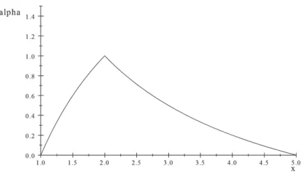
Note that for 0 ≤ α ≤ 1, the interval −α+5−α+3,α+3α+1 is proper. Moreover, the function −α+5−α+3 is increasing with α and the function α+3α+1is decreasing, which results in the following genuine fuzzy interval solution (Fig. 2). Case 4: United solution:
The fuzzy set extension of this case can be written as requiring that the fuzzy set ˜ax ∩ ˜b with membership function min(µ˜ax, µb˜)be a normal fuzzy set (intersecting cores), and we try to find the united solution for all cuts. It comes down to
[ ˜a(α) ˇx ∩ ˜b(α) 6= ∅, ∀α ∈ (0, 1] m
min ˜a(α)x ≤ max ˜b(α)and min ˜b(α) ≤ ˜a(α)x
It reads (α + 1)x ≤ −α + 5 and α + 3 ≤ (−α + 3)x, in other terms: α +3
−α + 3≤ x ≤
−α + 5 α +1
which results in the following genuine fuzzy set solution (Fig. 3).
It should be noted that the “there-exists-for-all”, Ä∃∀solution is contained in the “there-exists-there-exists”, Ä∃∃solution as expected. Since this is a one dimensional case, the NLV [Ä] solutions are the Ä solutions.
The following examples indicate that the robust solution of Case 1 may lead to cuts of the solution set that are not nested or even nested in the wrong direction, which prevents its interpretation as a fuzzy set.
Example 7. Suppose symmetric linear fuzzy intervals where ˜a has support [2, 12] and core {7}, and ˜bhas the same support as ˜a but a wider core [5, 9] The cuts are of the form ˜a(α) = [2 + 5α, 12 − 5α] and ˜b(α) = [2 + 3α, 12 − 3α].
Fig. 3. Fuzzy united solution Ä∃∃.
Clearly the Case 1 equation for cuts is of the form [2 + 5α, 12 − 5α]x ⊆ [2 + 3α, 12 − 3α]
which has solutions for all α > 0 of the form ˇx(α) = [2+3α2+5α, 12−3α12−5α]. The solution is such that ˇx(1) = [5/7, 9/7] and at the limit, ˇx(0) = {1}. Clearly the function 2+3α2+5α is decreasing with α and the function 12−3α12−5α is increasing, which is the opposite of what is hoped for fuzzy set cuts. If we interpret 1 − α as the level of confidence that a ∈ ˜a(α) and that ˜b(α) is the proper tolerance constraint, we see that the imprecision of the description of the information about parameter a considerably increases when the confidence requirement is relaxed (reaching a plausible value 7) while the tolerance range remains significant. It provides some degree of freedom for the choice of x, if we are lenient about confidence. On the contrary, if we require full safety about the value of a, then its imprecision range equates the tolerance range so that the only possible decision is x = 1. So the interpretation of this gradual set solution looks plausible anyway.
5.3. Connection with fuzzy relational equations
Note that the above examples have to do with elementary fuzzy interval equations studied independently by several scholars since the 1980’s; among other ones, for instance [6,14,62,63,77]. Especially, Sanchez[63]pointed out the connections of the robust formulation (Cases 1 and 2) with the fuzzy relational equations that he was the first scholar to study. To see it, it is clear that the equation ˜A ˇx ⊆ ˜bcan be written by means of the extension principle as follows:
sup A,x:b=Ax
min(µ[A]x(Ax), µxˇ(x)) ≤ µ[b](b), ∀b
a fuzzy relational equation of the form R ◦ ˇx ⊆ [b], where ◦ is the max min composition, and µR(A, x) = µ[A]x(Ax), whose solution is known to be of the form
µ1xˇ(x) =inf
b,Aµ[A]x(Ax) →Gµ[b](b), (25)
where r →Gs =1 if r ≤ s and s otherwise (Goedel implication). Indeed min(µ[A]x(Ax), µxˇ(x)) ≤ µ[b](b)if and only if µxˇ(x) ≤ µ[A]x(Ax) → µ[b](b). Note that this expression yields a genuine (possibly subnormalized) fuzzy set, contrary to the set of solution sets obtained by solving Case 1 equations for all α-cuts. In fact, systems of fuzzy linear equations can be cast in a more general fuzzy set-theoretic algebraic setting involving t-norms, and co-norms and residuated implications[31].
5.4. The possibilistic approach
Besides, when moving from the crisp interval linear system problem to the fuzzy linear interval problem, there are even more extensions of the equality between scalars than what we have presented here. We want to emphasize that,