O
pen
A
rchive
T
OULOUSE
A
rchive
O
uverte (
OATAO
)
OATAO is an open access repository that collects the work of Toulouse researchers and
makes it freely available over the web where possible.
This is an author-deposited version published in :
http://oatao.univ-toulouse.fr/
Eprints ID : 18474
To link to this article : DOI:10.1103/PhysRevE.96.033103
URL :
http://dx.doi.org/10.1103/PhysRevE.96.033103
To cite this version : Renaudière de Vaux, Sébastien and Zamansky,
Rémi and Bergez, Wladimir and Tordjeman, Philippe and Haquet,
Jean-François Destabilization of a liquid metal by nonuniform Joule
heating. (2017) Physical Review E, vol. 96 (n° 3).
pp.033103/1-033103/10. ISSN 2470-0045
Any correspondence concerning this service should be sent to the repository
administrator:
[email protected]
Destabilization of a liquid metal by nonuniform Joule heating
Sébastien Renaudière de Vaux,1,2 Rémi Zamansky,1 Wladimir Bergez,1 Philippe Tordjeman,1,* and Jean-François Haquet2
1Institut de Mécanique des Fluides de Toulouse (IMFT), Université de Toulouse, CNRS-INPT-UPS, Toulouse, France 2CEA, DEN, Cadarache, SMTA/LPMA, F13108 St Paul lez Durance, France
We study the effect of an impressing AC magnetic field at the bottom of a liquid metal layer of thickness h. In this situation the fluid is set in motion by the buoyancy forces caused by internal heat sources. The heat sources, caused by the Joule effect induced by the AC field, present an exponentially decaying profile, with characteristic length δ. As the magnetic field is horizontal, the Lorentz force has no influence on the dynamics of the system since it contributes only to the magnetic pressure. We propose an analysis of both the transient and fully developed regimes using linear stability analysis (LSA) and direct numerical simulations (DNSs). The transient period is governed by the temporal evolution of the temperature field as well as the development of the convective instability, which can be concomitant and therefore requires adopting a transient LSA algorithm to track these two effects. The DNSs have been performed for various distributions of the heat sources and various total heat input. This corresponds to independently varying δ/h in the range 0.04 6 δ/h 6 0.45 and a Rayleigh number 1.1×1046 Ra 6 1.2×10⁵. We observe the relaxation of the temperature up to the steady conductive profile before the transition to the nonlinear regime when Ra is small, whereas for larger Ra, nonlinear effects appear during the relaxation of the temperature profile. The unsteadiness of the temperature field significantly alters the development of the instability because of a much smaller growth rate. Surprisingly, we observe that δ/h has only a limited influence on averaged quantities as well as on the patterns for both the linear and nonlinear regimes. This comes with the fact that the profiles present an apparent reflectional symmetry, despite the asymmetry of the governing equations. DOI:10.1103/PhysRevE.96.033103
I. INTRODUCTION
When a liquid layer is confined between two horizontal walls, natural convection can occur in two different cases: on the one hand, when a temperature difference is applied between the two walls, this case corresponding to the conditions of Rayleigh-Bénard convection (RBC) and widely studied in the literature [1–3], and on the other hand, when temperature gra-dients in the liquid layer result from an internal heating. This latter case is encountered in many practical applications, such as metallurgy [4] and nuclear safety [5], chemical engineering, or the nuclear industry [6]. Here the internal heat sources are produced by magnetic induction (the Joule effect), chemical reactions, and nuclear disintegrations, respectively. Compared to RBC, the theory of convection resulting from an internal heating has received less attention, despite the importance of industrial applications. In this situation, the convection appears quickly during the transient diffusion of the temperature field. To understand how the transient temperature is coupled to the fluid dynamics, we consider, in this paper, both linear stability analysis (LSA) with a transient base state for the temperature and velocity fields, and direct numerical simulations (DNSs). In the case of horizontal layers subject to uniform internal sources, the Rayleigh number Ra can be defined proportionally to the heating rate (in K/s). The marginal stability of this case has been investigated by Sparrow et al. [7] using the steady conductive profile as the base state to compute the critical Rayleigh number Rac. For a fluid at rest, the establishment
of this profile is governed by the characteristic heat diffusion time τκ = h2/κ, with h a characteristic length and κ the fluid
thermal diffusivity. Note that in physical systems, this
charac-*[email protected]
teristic time can be τκ = O(103s). This, combined with large
Ra numbers, implies that the intermediate steady conductive profile may never be reached: the onset of convection appears simultaneously with the transient heat conduction. In that event, the transient conduction has to be taken into account in linear stability analysis in order to understand the transient flow development. It was indeed shown by Kolmychkov et al. [8] that the patterns in the transient regime significantly differ from the patterns in the established regime.
Aside from the transient aspects, we consider the influence of the distribution of the thermal source term. Actually the internal sources are rarely uniform, and in the case of induction heating by an AC magnetic field, the source terms concentrate in the skin depth δ =√2η/ω, with η the magnetic diffusion coefficient and ω the pulsation of the magnetic field. Here we consider the effect of a high-frequency harmonic magnetic field (δ/h < 1) of amplitude B0 imposed at the bottom of a
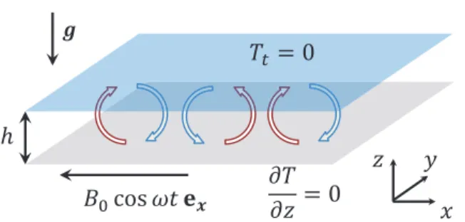
horizontal fluid layer of liquid metal, as depicted in Fig.1. The diffusion of the magnetic field induces electric currents directly inside the fluid and a Lorentz force. However, with this config-uration of the magnetic field, due to B · ∇B = 0, the Lorentz force has only a contribution through the magnetic pressure. This contrasts with RBC in the presence of DC magnetic fields, where the Lorentz force has a stabilizing role [9,10]. The heat source decays exponentially with z over a characteristic scale δ/2h. For this configuration, Tasaka and Takeda [11] analyzed the marginal stability of the flow. They showed that increasing δ/ hslightly increases the marginal stability criterion and hence tends to delay convection. In the present paper, we observe that, in both the linear and nonlinear regimes, the pattern dynamics present a great similarity irrespective of the geometry of the energy deposition (keeping the total energy input constant). Moreover, except in the very early transient period, the flow presents an apparent reflectional symmetry about the
FIG. 1. Studied configuration: an unbounded horizontal layer of liquid metal confined by two walls. The bottom wall is insulating, and the top wall is a perfect conductor. g is the acceleration of gravity. For the DNS, the infinite extent of the domain is approximated by periodic boundary conditions.
horizontal midplane contrary to the governing equations. This result departs from the numerical and experimental results for the steady regime of homogeneously internally heated layers (see Ref. [12] for a review). In particular, for 1066 Ra 6 1010
[as defined below in (20)], Goluskin and van der Poel [13] showed that velocity profiles are not symmetrical.
The paper is organized as follows. In Sec.IIwe present the geometry, the characteristic scales of the problem, and the equations with boundary conditions. In Sec.IIIthe numerical results obtained by the DNS approach are presented. The LSA method around a transient base temperature field is introduced in Sec.IValong with the analysis of the linear regime. Final analysis and discussion are provided in Sec.V.
II. FORMULATION OF THE PROBLEM
We consider a horizontal layer of height h of an electrically conducting fluid, initially at the same temperature as the surroundings. This layer is subjected to gravity −gezand to a
horizontal AC magnetic field of amplitude B0imposed at the
bottom wall, as described in Fig.1. In this study, we use the thermal diffusion time τκ= h2/κas the reference time scale.
The layer is infinitely wide in (x,y) directions. The bottom wall is electrically and thermally insulating. At the top, we assume a perfect thermal and electrical conductor. In addition, we consider that the characteristic magnetic diffusion time τη =
h2/ηis much smaller than the advective time and the viscous and thermal diffusion times. These conditions correspond to small magnetic Reynolds Rm = Uh/η, and Prandtl Pm = ν/η numbers hypothesis, with U a characteristic velocity and ν the kinematic viscosity. We assume constant physical properties of the fluid, and the order of magnitude of the thermal and magnetic Prandtl numbers corresponding to liquid metal as gallium [14,15] are Pr = ν/κ = 0.025 and Pm = 1.55×10⁻⁶.
As Rm ≪ 1 is considered, the nondimensional equations for the electromagnetic field are independent of the velocity field and are given by
∂B ∂t = Pr Pm △B, (1) j = δ h∇ × B, (2) ∇ · j = ∇ · B = 0, (3) B(z = 0,t) = cos ωt ex, B(z = 1,t) = 0, (4)
where j is the electric current density scaled by j0= B0/µ0δ,
and ω is the nondimensional pulsation.
Equation (4) corresponds to the boundary conditions for the magnetic field. All the Cartesian coordinates are scaled by the thickness h. The solution of this system, as obtained by Fourier expansion, is given by
B = " cos(ωt)[1 − z] + ∞ X n=1 (α1,n+ α2,n) sin(λnz) # ex, (5) j = δ h " − cos(ωt) + ∞ X n=1 λn(α1,n+ α2,n) cos(λnz) # ey, (6) where α1,n= 2ω λn ( £ λ2nsin(ωt) Pr±Pm−ω cos(ωt)¤+ω e−λ2ntPr/Pm ¡ λ2nPr±Pm¢2+ω2 ) , (7) α2,n= 2 λn e−λ2ntPr/Pm, (8) with λn= nπ.
Owing to the large Pr/Pm ratio, the exponential terms in (5) and (6) are vanishingly small, and one can assume that the profiles of the magnetic induction and electric current are instantaneously established.
In line with the inductive heating applications [16], we consider only very small periods of the AC magnetic field: ω ≫ 1. As a consequence of the high frequency of the applied magnetic field, we can consider the Joule effect and Lorentz force averaged over a time τa much larger than the period
of the magnetic forcing and much smaller than the other relevant time scales of the flow. In this limit one obtains the magnetohydrostatic approximation [17]. When normalized by j2
0/σ, the time-average power deposited in the liquid is
given by hj2i = τ1 a Z t +τa t j2(t′) dt′. (9)
In the δ/h ≪ 1 limit, it can be shown that the solution for hj2
i from Eq. (6) reduces to
hj2i = exp µ
−δ/ h2z ¶
, (10)
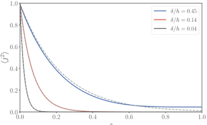
which corresponds to exponentially decaying source term [16]. Figure2compares hj2
i computed from Eq. (6) and obtained in the semi-infinite limit (10), for δ/h = 0.45, 0.14, and 0.04. As it can be observed, (10) gives a good approximation of the energy distribution in the liquid volume even for δ/h = 0.45. We now introduce the nondimensional average power Ŵ =R01hj2i dz. Its value is given by the spatial distribution
of the heat sources. In the δ/h ≪ 1 limit, Ŵ reduces to Ŵ = 2hδ
·
1 − expµ −2hδ ¶¸
0.0 0.2 0.4 0.6 0.8 1.0 z 0.0 0.2 0.4 0.6 0.8 1.0 j 2 δ/h = 0.45 δ/h = 0.14 δ/h = 0.04
FIG. 2. Nondimensional Joule term (solid lines) profile computed from averaging Eq. (9). The dashed lines represent the semi-infinite solution given by Eq. (10).
The power input caused by Joule effect concentrates in the region of thickness δ close to the bottom wall. This, in turn, generates buoyancy forces that could lead to fluid motion. In the case of standard RBC inception for liquid metals (small Pr), the conduction equilibrium temperature profile is reached before destabilization [9]. This is in contrast with the present study, where the rate of heat deposited in the volume, coupled with the adiabatic condition at the bottom wall, is observed to cause destabilization before the thermal conduc-tion equilibrium state is reached. This motivates us to derive the transient temperature profile T0(z,t) driven by thermal
conduction, i.e., without convection. The nondimensional heat conduction equation with boundary conditions and isothermal initial conditions are
∂T0 ∂t = △T0+ 1 Ŵhj 2 i, (12) ∂T0 ∂z (z = 0,t) = 0, T0(z = 1,t) = 0, T0(z,t = 0) = 0. (13) The characteristic temperature difference is defined, similarly to Ref. [13], as 1T =Ŵτκj 2 0 ρcpσ , (14)
where ρ is the density, cp is the specific heat capacity of the
liquid metal, and σ its electrical conductivity. Assuming that hj2i and Ŵ obey (10) and (11), the steady-state temperature solution is T∞(z) = 1 Ŵ · −(δ/h) 2 4 exp µ −2z δ/ h ¶ + az + b ¸ , where a = −2hδ and b = 2hδ · 1 +2hδ exp µ −2hδ ¶¸ . (15) Note that with the choice of 1T (14), the heat balance imposes dT∞/dz = −1 at z = 1. The transient temperature field is
T0(z,t) = T∞(z) − T′(z,t), where T′(z,t) = ∞ X n=1 [31,n+ 32,n+ 33,n] × cosµ 2n − 1 2 π z ¶ × exp µ −2n − 12 π t ¶ , (16) and 31,n= −2µ δ 2h ¶2 2δ h + (−1) nζ n ¡δ 2h ¢2 exp(−2h/δ) ¡δ h ¢2 ζn2+ 4 , (17) 32,n= 2a ζn(−1)n− 1 ζn2 , (18) 33,n= 2b(−1) n ζn , (19)
with ζn= (2n − 1)π/2. We note that the fluid temperature
difference between the top and bottom scales as 1T and corresponds to the maximum temperature in the liquid layer. This scale is used to define the Rayleigh number Ra:
Ra = gβ1T h3/νκ. (20) The convective motions are described by the Navier-Stokes system in the Boussinesq approximation and the magnetohy-drostatic approximation [17]: ∂u ∂t + (u · ∇)u = −∇p ⋆ + Pr △ u + Ra Pr T ez, (21) ∇ · u = 0, (22) ∂T ∂t + (u · ∇)T = △T + 1 Ŵhj 2 i, (23)
where u = (U,V,W) is the fluid velocity in units of κ/h, T is the fluid temperature normalized by 1T , and p⋆is the pressure
supplemented by the magnetic pressure in units of ρ(κ/h)2.
The boundary conditions for the temperature are the same as in (13), and we impose no-slip boundary conditions for the velocity. Moreover, all the physical quantities in (21)–(23) are averaged over τa as in (9). It is to note that due to the
presence of a thermal source term in (23), the system does not have the reflectional symmetry about the midplane, contrary to the classical RBC configuration within the Boussinesq approximation [18,19]. Also, the difference between the top and bottom walls for thermal boundary conditions participates in the asymmetry.
The nondimensional numbers that appear in the set of Eqs. (21)–(23) are δ/h (through Ŵ), Pr, Pm, and Ra. We will study the effects of varying the two main nondimensional parameters Ra and δ/h while keeping the other parameters constant.
III. RESULTS FROM THE DIRECT NUMERICAL SIMULATIONS
We solve Eqs. (21)–(23) by direct numerical simulation (DNS) with the finite volume code Jadim [20] with the prescribed profile of hj2
TABLE I. Studied points Pr = 0.025, Pm = 1.55×10⁻⁶. The ratio δ/h is the relative skin depth, Ra is the Rayleigh number, s(t = ∞) is the growth rate calculated by LSA with T0= T∞, and kmaxis the nondimensional wave number in the steady regime.
δ/ h 0.45 0.14 0.14 0.14 0.04 0.04
Ra 1.1×10⁴ 1.1×10⁴ 3.7×10⁴ 1.2×10⁵ 1.1×10⁴ 1.2×10⁵
Ŵ 0.216 0.070 0.070 0.070 0.022 0.022
s(t = ∞) 3.51 4.12 12.1 28.9 4.19 29.4
kmax 3.20 3.33 3.80 4.50 3.20 4.44
given in Fig. 2. The code uses a third order Runge-Kutta scheme for temporal integration. The spatial derivatives are calculated with second order accuracy. The incompressibility is achieved through a projection method. The viscous terms are calculated using a semi-implicit Crank-Nicolson scheme. The case is solved in a biperiodic box of aspect ratio 10 (see Fig.1), with Nx×Ny×Nz= 512×512×128. This mesh
is chosen to satisfy the criteria from Grötzbach [21]. We have checked that the numerical results are independent of a further refinement of the numerical mesh. In particular, we have compared two numerical simulations in a box with aspect ratio 1, for 1283 and 2563 grid points at Ra = 1.2×10⁵ and
δ/ h = 0.04. We observe that both velocity and temperature profiles are identical, and integral quantities agree within an error of 1%. For all simulations the initial conditions are given by uncorrelated random velocity and temperature fields with zero mean and a nondimensional amplitude of 10−9.
We investigate the effect of both the heterogeneity and the intensity of the source term. For that, we studied by DNS six cases presented in Table I. We compare three cases at the same Ra = 1.1×10⁴ and δ/h = 0.04, 0.14, and 0.45;
two cases at the same δ/h = 0.04 and Ra = 1.1×10⁴ and
1.2×10⁵; and three cases at the same δ/h = 0.14 and Ra =
1.1×104,3.7×104, and 1.2×10⁵. In all those simulations
we set Pr = 0.025, Pm = 1.55×10⁻⁶. In our configuration,
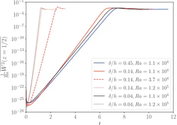
because of the invariance of B in the horizontal directions, the Lorentz force contributes only through Maxwell pressure. As a consequence, the set of parameters studied can be understood as varying the magnitude and pulsation of the applied magnetic field. 0 2 4 6 8 10 12 t 10−28 10−25 10−22 10−19 10−16 10−13 10−10 10−7 10−4 10−1 1WRa 2(z = 1/ 2) δ/h = 0.45, Ra = 1.1 × 10⁴ δ/h = 0.14, Ra = 1.1 × 10⁴ δ/h = 0.14, Ra = 3.7 × 10⁴ δ/h = 0.14, Ra = 1.2 × 10⁵ δ/h = 0.04, Ra = 1.1 × 10⁴ δ/h = 0.04, Ra = 1.2 × 10⁵
FIG. 3. Time evolution of kinetic energy. Both time and kinetic energy are normalized by the thermal diffusion scale.
We first present the temporal evolution of the kinetic energy in the system. In Fig.3, we consider the following quantity as characteristic of the kinetic energy, which is directly given by LSA: W2(z = 1/2) = 1 A Z Z A W2(z = 1/2) dx dy, (24) with A the area of the wall. We observe that all the curves present the same behavior. Due to the small magnitude of the initial fields, the early dynamics can be considered linear, as long as nonlinear convective terms remain vanishingly small. But the rate of variation of the kinetic energy, defined as
s(t) =1 2
d dt log[W
2(z = 1/2)], (25)
presents a nontrivial evolution. In the first moments, one observes a decrease of the kinetic energy, followed by a quasiexponential growth of the kinetic energy. The dependence of s(t) with time is caused by the transient development of the temperature profile. The initial temperature gradients are not large enough to set the fluid in motion and the initial perturbation is damped. Then the temperature gradient becomes sufficiently large for the Rayleigh instability to develop. The last stage observed in Fig. 3 is a steady-state regime in which W2∼ Ra, as expected from general scaling
theories in thermal convection [22], and as obtained with DNS for DC magnetic fields [9]. We note that, for a purely conductive heat flux in (12), the transient period of the temperature is of the order of τκ (or t = 1 with our choice
of normalization). As seen in Fig.3, for the largest Rayleigh numbers the steady-state regime is reached for t ≈ 1, meaning that in such cases, the conductive equilibrium temperature T∞ in (15) is never reached.
For all cases, the convection significantly influences the temperature profiles of the steady-state regime, as seen in Fig. 4, where those profiles are compared with T∞ for the various δ/h. As the heat flux is fixed at the upper wall by the heat balance in the liquid, the average temperature gradient at z = 1 in the steady state is equal to −1 (according to the temperature scaling). As a consequence the bottom (adiabatic) wall temperature decreases with Ra for a same δ/h. Also observed in Fig.4, increasing Ra induces a more homogeneous temperature in the liquid, which corresponds to an approximate uniform temperature in the liquid core. Finally, it is observed that the value of δ/h has a mild effect on the temperature profile. At δ/h = 0.45, we observe a regular temperature profile, with a monotonous evolution of the mean temperature gradient dT /dz, while for δ/h = 0.04 and 0.14 at the same Ra, the evolution is more complex with a shape reminiscent of a sigmoid function.
0.0 0.2 0.4 0.6 0.8 1.0 z 0.0 0.2 0.4 0.6 0.8 1.0 T δ/h = 0.45 Ra = 1.1 × 10⁴ δ/h = 0.14 Ra = 1.1 × 10⁴ Ra = 3.7 × 10⁴ Ra = 1.2 × 10⁵ δ/h = 0.04 Ra = 1.1 × 10⁴ Ra = 1.2 × 10⁵
FIG. 4. Time and (x,y) direction averaged temperature profiles for the three Ra in the steady-state regime. The circles represent T∞ from (15) for δ/h = 0.45 (blue), 0.14 (red), and 0.04 (black).
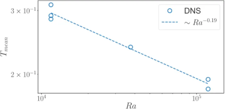
For homogeneous heating Goluskin and van der Poel [13] showed that the nondimensional mean temperature Tmean=
1 V
R
VTdV scales as Tmean∼ Ra−1/5, with V the volume of
the layer. Figure5presents the plot of Tmeanas a function of
Ra for all our DNS. First, consistently with the smallness of the δ/h effect on the T profiles, it is observed that the points for the different δ/h are quasisuperimposed for a given Ra. Furthermore, we observe that the scaling proposed in Ref. [13] remains valid even if, in our case, the heating is concentrated in the skin layer.
Figure 6 presents the normalized averaged profiles of tangential velocitypU2+ V2 and vertical velocitypW2 in the nonlinear steady-state regime, for all the cases in TableI. We observe in this figure that all velocity profiles are nearly symmetrical about the midplane, with in particular the same boundary layers on both top and bottom walls [Fig. 6(a)] and maximum vertical velocity at z = 1/2 [Fig. 6(b)]. This apparent symmetry is surprising since, in contrast with the standard RBC for which a temperature difference is imposed on the wall, due to the source term and the different boundary conditions, Eqs. (21)–(23) are not invariant with this symmetry.
104 105 Ra 2 × 10⁻¹ 3 × 10⁻¹ Tm ea n DNS ∼Ra−0.19
FIG. 5. Tmeanvs Ra. The dashed line is a linear fit of the data.
0.0 0.2 0.4 0.6 0.8 1.0 0.00 0.25 0.50 0.75 1.00 U 2+ V 2/max U 2+ V 2 (a) 0.0 0.2 0.4 0.6 0.8 1.0 z 0.00 0.25 0.50 0.75 1.00 W 2/ max W 2 (b) δ/h = 0.45 Ra = 1.1 × 10⁴ δ/h = 0.14 Ra = 1.1 × 10⁴ Ra = 3.7 × 10⁴ Ra = 1.2 × 10⁵ δ/h = 0.04 Ra = 1.1 × 10⁴ Ra = 1.2 × 10⁵
FIG. 6. Average over time and (x,y) direction of (a) the velocity tangential to the wallspU2+ V2 and of (b) the vertical velocity magnitudepW2.
Additionally, the comparison of the normalized velocity profiles in the steady state does not show significant difference although the volume of energy deposition varies strongly with the layer thickness δ/h. As seen in Fig.3 the velocity magnitude scales as √Ra (in the steady state). Owing to the large value of (Ra − Rac)/Rac≈ 10–100 imposed in our
simulations, the convection efficiently homogenized the tem-perature fluctuations and cancels out the transient effects and the geometry of energy deposition at long time. This causes the weak dependence in δ/h. Moreover, the profiles of horizontal and vertical velocities are correlated; a maximum vertical velocity corresponds to a minimum of the horizontal velocity. However, this minimum is not very pronounced, indicating that the convection in the cell core is three-dimensional. Increasing Ra tends to reduce the boundary layer thickness and to broaden slightly the vertical velocity profiles.
For a constant Ra = 1.1×10⁴ and the three values of
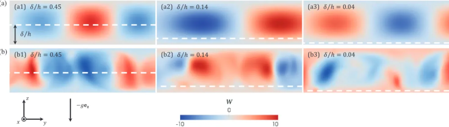
the penetration depth, Fig.7 compares the vertical velocity patterns in the linear regime and in the steady-state regime. The snapshots show the presence of convective cells in the linear regime similarly to RBC. These cells are symmetrical about the z = 1/2 plane. In the nonlinear regime, the cells disappear and evolve to irregular patterns with smaller unsteady structures (Fig. 7). However, there is no clear effect of δ/h on the instantaneous velocity fields: the same color scale is used for the three values of δ/h and qualitatively the same patterns are observed. In this regime, the structures fluctuate intensively along with a broadening of the velocity spectrum.
For Ra = 3.7×10⁴, the cells of the linear regime are
characterized by a nondimensional wave number k ≈ 3.8 constant during the linear regime, as seen in Fig.8. This wave
(a)
(b)
FIG. 7. Color maps of instantaneous W velocity (red is upward and blue is downward) in a plane parallel to gravity at Ra = 1.1×10⁴(a) in the linear regime and (b) in the steady regime. The horizontal dashes show the skin depth: (a1 and b1) δ/h = 0.45, (a2 and b2) δ/h = 0.14, and (a3 and b3) δ/h = 0.04. The width of each panel is 1/3 of the total width. The top panels are normalized by the instantaneous W amplitude, and the bottom panels share the same color scale indicated in panel (b).
number is also observed to be independent of δ/h. When Ra increases, we observed from our DNS that k increases and tends to a value k ≈ 4.5. At the end of the linear regime the DNS shows a broadening of the horizontal spectrum of the vertical velocity. We can assume that this broadening is due to the inertia term coupled with three-dimensional effects. At the transition between the linear and the steady-state regime, the spectrum broadens. In the nonlinear regime the energy spectral density (ESD) for k > 5 is superimposed with the ESD at the maximum kinetic energy, but the main peak is located around k ≈ 2.6. We observe a similar behavior for all cases studied by DNS.
IV. LINEAR STABILITY ANALYSIS
We use the adjoint method to solve the LSA [23]. Indeed, for short time t . 1, the linear operators are time dependent due to the transient temperature field in the medium. Here the initial state is u(x,t = 0) = 0 and T (x,t = 0) = 0. The velocity perturbation υ(x,t) is defined relatively to the zero-velocity base state. The temperature perturbation ϑ(x,t) is
0.0 2.5 5.0 7.5 10.0 12.5 15.0 17.5 20.0 k 0.0 0.1 0.2 0.3 0.4 0.5 0.6 0.7 E S D t = 1.26, k 3.8 t = 2.58, k 3.8 t = 3.18, k 2.6
FIG. 8. Normalized energy spectral density (ESD) for the case δ/ h = 0.14 and Ra = 3.7×10⁴ in the linear regime (blue), at maximum kinetic energy (orange), and in the stationary regime (green). The wave number k in the legend indicates the main peak location.
defined relatively to the purely conductive temperature profile which evolves with time. This base state transient temperature profile T0(z,t) is given by (12) and (13). This is in contrast
with usual linear stability studies, where the base profile is assumed to be given by the steady conduction solution (u,T ) = (0,T∞) (see, for example, Refs. [9,11,16]). In this study, this equilibrium state is not systematically reached because the onset of convection appears during thermal relaxation.
Following Refs. [9,24], we consider only the perturbation of the velocity in the vertical direction w. At first order, (w,ϑ) is governed by ∂△w ∂t = Pr △ 2 w + Ra Prµ ∂ 2ϑ ∂x2 + ∂2ϑ ∂y2 ¶ , (26) ∂ϑ ∂t = △ϑ − w dT0(z,t) dz . (27)
Equation (26) is the linearized z component of −∇×∇× (21). Here, the pressure p⋆ in (21) does not appear in Eq. (26)
because this force is irrotational and does not contribute to the instability development. Note that in (27), the Joule effect is included in the evolution of T0(z,t). Considering disturbances
as two-dimensional waves in the horizontal plane, with wave vector k = (kx,ky), we obtain µ w ϑ ¶ = µ w0(k; z,t) ϑ0(k; z,t) ¶ | {z } X(k;z,t) exp i(kxx + kyy). (28)
Here w0(k; z,t) and ϑ0(k; z,t) are the perturbation amplitudes
corresponding to the k mode. Equations (26) and (27) can be put in the form of a nonautonomous linear system:
L1
dX
dt = L2(t)X, (29) with the operators
L1=µPr (D 2 − k2) 0 0 1 ¶ and (30) L2(t) =µPr (D 2 − k2)2 −Ra Pr k2 −DT0(t) (D2− k2) ¶ , (31)
with D ≡ d dz and k
2
= kx2+ k 2
y. In this differential system
only the L2 operator is time dependent. Following the same
boundary conditions as for DNS, we consider an infinitely thermally conducting wall on the top and an insulated bottom wall. The boundary conditions, following the no-slip conditions, continuity, and thermally insulating or conducting walls are
w0= Dw0= Dϑ0= 0, for z = 0, (32)
w0= Dw0= ϑ0= 0, for z = 1. (33)
Following the adjoint method, the eigenvectors ˆXn, their
adjoint ˆX†
m, and the corresponding eigenvalues λnand λ † mare
given by the following system:
λnL1ˆXn= L2ˆXn,
λ†mL1ˆX†m= L †
2ˆX†m, (34)
where L†
2 is the adjoint of L2. Due to the non-normality of
the system, ( ˆXn)n∈N and ( ˆX †
m)m∈N form two nonorthogonal
basis. The condition of orthogonality is here defined by the identity (L1ˆXn| ˆX
†
m) = δnm, where δnm is the Kronecker
symbol. This orthogonality condition also imposes λn= λ † n
for real eigenvalues.
For each k mode, the perturbation amplitude can be decomposed on the eigenvectors basis:
X(k; z,t) =X n αn(k; t) ˆXn(k; z,t), (35) with dαn dt = λn(t)αn− X m µ L1d ˆXm dt ¯ ¯ ¯ ¯ˆX † n ¶ αm. (36)
Equation (36) is obtained by substituting (35) into (29) and using the orthogonality of the direct and the adjoint modes (34). From (36), we see that the amplitude growth is due to (1) the instability of the mode n (λn>0) and (2) the time
dependence of the base state (d ˆXm/dt 6= 0). It implies that
the coupling between the variations of all the eigenvectors can participate in the growth of the unstable k mode for t . 1. When t ≫ 1, this coupling vanishes, and the most unstable kmode grows exponentially with the asymptotic growth rate λn(t → ∞).
To solve the system (34), we approximate the operators L1,L2, and L†2 with second order finite difference schemes.
Details on the numerical schemes can be found in Ref. [9]. To obtain the velocity profile, the perturbations w0(k; z,t) are
summed up over for Nk= 48 linearly spaced wave numbers
between 0 < k < 10. Here we used Nz= 256 grid points. We
checked that further increases in Nzand Nkhad no influence
on the results.
The z component of the velocity field is thus obtained as W(x,t) =
Z Z
w0(k; z,t) exp i(kxx + kyy) dkxdky. (37)
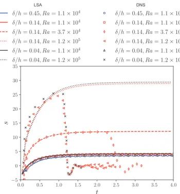
This enables us to compute the growth rate of the perturbation s(t) =12dlog Wdt 2 in order to compare with the DNS. Figure9 presents the evolution of s(t) obtained from the DNS and
0.0 0.5 1.0 1.5 2.0 2.5 3.0 3.5 4.0 t −5 0 5 10 15 20 25 30 35 s LSA δ/h = 0.45, Ra = 1.1 × 10⁴ δ/h = 0.14, Ra = 1.1 × 10⁴ δ/h = 0.14, Ra = 3.7 × 10⁴ δ/h = 0.14, Ra = 1.2 × 10⁵ δ/h = 0.04, Ra = 1.1 × 10⁴ δ/h = 0.04, Ra = 1.2 × 10⁵ DNS δ/h = 0.45, Ra = 1.1 × 10⁴ δ/h = 0.14, Ra = 1.1 × 10⁴ δ/h = 0.14, Ra = 3.7 × 10⁴ δ/h = 0.14, Ra = 1.2 × 10⁵ δ/h = 0.04, Ra = 1.1 × 10⁴ δ/h = 0.04, Ra = 1.2 × 10⁵
FIG. 9. Comparison of s computed with LSA (lines) and DNS (symbols).
the LSA for all the DNS cases. It is seen that initially s presents negative values. The system is linearly stable because of the absence of the temperature gradient in the initial condition. Subsequently, s increases up to a constant value within a characteristic time τκ (equal to 1 with our choice of
normalization). A very good agreement between the results of DNS and LSA in the linear regime is observed. At the end of the linear regime, the growth rate from DNS falls to a minimum value before becoming zero on average in the nonlinear steady-state regime. For t ≫ 1, the LSA prediction for s converges to an asymptotic value. It is worth noticing that the evolution of s(t) appears to be independent of δ/h.
In Fig. 10we present the dependence of the asymptotic value of s with the parameters Ra and δ/h. It confirms that δ/ hhas little influence on the growth rate at first order in the range 0.03 < δ/h < 0.5. On the other hand, s is an increasing function of Ra. We observe that the marginal stability criterion is Rac≈ 1200, which is consistent with the computation
of Tasaka and Takeda [11]. We also present the result of the marginal stability for δ/h = 0 and δ/h → ∞ [12]. The limit δ/h = 0 corresponds to a system with bottom heating. The second limit δ/h → ∞ corresponds to a homogeneous heating. These results of the literature confirm the minor effect of δ/h on the convection, which has been observed by DNS for t > 1 and Ra > Rac.
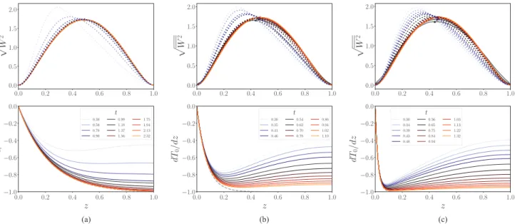
The time dependence of the vertical velocity perturbations calculated by LSA is presented in Fig.11 for t . 3, Ra = 1.1×10⁴and the three δ/h values. These profiles are compared
to those obtained by DNS for t > 0.50. The very good agreement between LSA based on the adjoint method, and DNS shows the two methods are consistent.
For all δ/h, we observe that the profile of the velocity perturbation is asymmetrical in the first moments and then
0.1 0.2 0.3 0.4 0.5 δ/h 103 104 105 106 R a marginal stability 0 40 80 120 160 200 240 s
FIG. 10. Contours of s(t = ∞) in the (Ra,δ/h) plane. The circles represent the DNS. The black line is the marginal stability. The gray triangle is the critical Rayleigh Rac(δ/h) computed by Tasaka and Takeda [11]. The gray squares correspond to the limiting cases δ/ h = 0 and δ/ h → ∞, as given by Goluskin [12].
evolves towards a symmetrical profile as time increases. This behavior is linked with the temporal evolution of the temperature gradient of the base state, dT0/dz. It is observed
in Fig. 11 that dT0/dz presents a local minimum close to
the bottom wall during the establishment of the stationary conductive temperature profile, which lasts for t = O(1). The position of the dT0/dzminimum moves closer to the lower
wall, and its amplitude increases as δ/h is decreased. The presence of a maximum temperature gradient magnitude in the volume is responsible for a local high buoyancy force, and consequently of the asymmetry of the velocity profile. Indeed, for δ/h = 0.45 the minimum is weak and the symmetry of the velocity profile restored quickly, whereas for δ/h = 0.04, there is a sharp local minimum and the asymmetry of the velocity perturbation is more persistent. For small Rayleigh
numbers regardless of the value of δ/h, the velocity profile becomes symmetrical before the end of the transient linear regime. For larger Ra, we observed that the nonlinear regime starts before that the steady conductive temperature profile T∞ is reached and therefore the symmetry of the velocity is not restored during the linear regime. As seen from (27), the source term is given by the product of the dT0/dzwith w, is
asymmetrical. Therefore at high Ra, the asymmetry of the base temperature profile has more impact on the perturbations. On the other hand, the advective transport of the temperature tends to homogenize the temperature fluctuations in the nonlinear regime.
V. DISCUSSION AND CONCLUSION
In this work, we studied the thermal convection of a liquid metal under AC magnetic field by DNS and LSA. Here, the two control parameters are the Rayleigh number Ra characteristic of the deposited power, and the nondimensional skin depth δ/h, which represents the power spatial distribution. Physically, these parameters can be tuned through the magnetic field amplitude B0and pulsation ω. In this study, we realized
DNS for three δ values smaller than half of the liquid thickness. The two important scales that govern the thermal convection are the temperature and the time scales, 1T and τκ. 1T
that fixes Ra is a function of ω and the power applied to the liquid. In opposition to the thermal convection under a DC magnetic field, imposing a horizontal AC magnetic field has no additional stabilization effect since only the magnetic pressure contributes to the Lorentz force. For all cases, we observe two flow regimes, a linear one and a nonlinear one. According to (25), the growth rates of the kinetic energy s(t) computed by LSA are compared to DNS in Fig.9. In LSA and for all the cases, s increases to a constant value with a characteristic time which is trivially equal to τκ, the characteristic time of heat
diffusion. We observe a very good agreement between the
0.0 0.2 0.4 0.6 0.8 1.0 0.0 0.5 1.0 1.5 2.0 W 2 0.0 0.2 0.4 0.6 0.8 1.0 z −1.0 −0.8 −0.6 −0.4 −0.2 0.0 dT 0 /dz t (a) 0.0 0.2 0.4 0.6 0.8 1.0 0.0 0.5 1.0 1.5 2.0 W 2 0.0 0.2 0.4 0.6 0.8 1.0 z −1.0 −0.8 −0.6 −0.4 −0.2 0.0 dT 0 /dz t (b) 0.0 0.2 0.4 0.6 0.8 1.0 0.0 0.5 1.0 1.5 2.0 W 2 0.0 0.2 0.4 0.6 0.8 1.0 z −1.0 −0.8 −0.6 −0.4 −0.2 0.0 dT 0 /dz t (c)
FIG. 11. Evolution of velocity profiles (top panel, DNS: lines; LSA: circles) and temperature gradients computed from (15) and (16) (bottom panel), for (a) δ/h = 0.45, (b) δ/h = 0.14 and (c) δ/h = 0.04 at Ra = 1.1×10⁴. The triangles in the top panel represent the maximum of√W2. The velocity profiles are normed by their integral. The dashed line is T∞from (15).
results of DNS and LSA in the linear regime. The growth rate calculated by DNS falls to a minimum value at the transition between linear and nonlinear regimes, and becomes zero in average in the nonlinear regime. We found that s(t) is independent of δ/h at constant Ra. Moreover, the asymptotic values of the growth rate predicted by LSA seem to be a linear increasing function of Ra. As a consequence, as long as the transition to a nonlinear regime occurs at t > 1 (i.e., for times larger than τκ), the kinetic energy grows as W2∼ exp[2s(Ra)t]
where s(Ra) is displayed in Fig.10. In the nonlinear regime, we recall that the kinetic energy scales in Ra, W2
∼ Ra, as observed in RBC and in thermal magnetoconvection with a constant magnetic field (small Rm).
The hydrodynamic patterns are classically studied by DNS. While LSA selects a main wave number that corresponds to a maximum growth rate, the DNS shows a widening of the wave number spectrum of the horizontal patterns (Fig.8). We can assume that this broadening is due to the inertial term coupled with three-dimensional effects. In the nonlinear regime we systematically observe that the wave number spectrum extends to large k values.
The transient dynamics of the system is determined (1) by the time dependence of the temperature field, which tends to relax from the isothermal to a purely conductive heat flux temperature profile T∞; (2) by the growth of the convective instability. In the linear regime, two behaviors are identified depending on the value of Ra. At small Ra, the growth rate of the instability is small enough to allow the relaxation of the temperature up to the steady conductive profile before the transition to the nonlinear regime. Conversely, for large Ra, the nonlinear effects appear for t < 1. This is in contrast with RBC and thermal convection with DC magnetic field, for which the thermal relaxation is usually much quicker than the develop-ment of the instability [9]. For usual liquid metals (gallium, sodium, bismuth, etc.) and for h of order 0.1 to 1m, the charac-teristic thermal diffusion τκvaries from 500 to 5000 s. In these
conditions, we expect that the transient dynamics is relevant for the study of the convection in the presence of magnetic fields. In the linear and nonlinear regimes, Eqs. (21)–(23) present reflectional symmetry when δ/h → 0. This symmetry
disappears when δ/h → ∞, which corresponds to homo-geneous heating. In these limiting cases, the solutions and consequently the dynamic patterns follow the equation sym-metry [13]. In this paper, we consider intermediate values of δ/ hfor which the equations are nonsymmetrical. For t ≪ 1 and in the linear regime, the solutions and the patterns are also nonsymmetrical (Fig.11). On the other hand, for t & 1 and independently of the flow regime, the solutions and the patterns are surprisingly symmetrical. In the linear regime, the conductive equilibrium temperature field is reached, and consequently the source term w dT0/dz is indeed almost
symmetrical because dT0/dz ≈ −1 except close to the walls
where w ≈ 0 (as seen in Fig.11). In the nonlinear regime, the symmetry of solutions is attributed to the relative importance of the temperature advection at large Ra, which mitigates the effect of the heterogeneous energy deposition.
If we compare the results between AC and DC magnetic fields, we observe large similarities of behavior, as a transition between linear and nonlinear regimes for a same scaling W2
∼ Ra. We also observe differences as Ra dependence on s in the linear regime, the presence of transient temperature base state, and the variety of patterns for DC magnetic field.
In perspective, a systematic study in the nonlinear regime is necessary to understand the dissipation mechanisms and the apparition of substructures. From a fundamental point of view, it is also interesting to address the transition from linear to nonlinear when t < 1 for which the steady-state conductive temperature field is not yet reached. Finally, the magnetohydrodynamic effects have no influence in this study. These effects can change the conclusions at large Rm.
ACKNOWLEDGMENTS
The present study is funded by the French Atomic Energy Commission (CEA) and the ECM Company. The work was granted access to high performance computing from Calmip (Project No. P0910) and Genci-Cines (Grant No. A0022B07400). The authors greatly acknowledge the help of Annaïg Pedrono for the numerical developments in the Jadim code.
[1] E. Bodenschatz, W. Pesch, and G. Ahlers, Recent developments in Rayleigh-Bénard convection,Annu. Rev. Fluid Mech. 32,709
(2000).
[2] G. Ahlers, S. Grossmann, and D. Lohse, Heat transfer and large scale dynamics in turbulent Rayleigh-Bénard convection,
Rev. Mod. Phys. 81,503(2009).
[3] D. Lohse and K. Q. Xia, Small-scale properties of turbulent Rayleigh-Bénard convection,Annu. Rev. Fluid Mech. 42,335
(2010).
[4] V. R. Gandhewar, S. V. Bansod, and A. B. Borade, Induction furnace—A review, Int. J. Eng. Tech. 3, 277 (2011).
[5] C. Journeau, P. Piluso, J. F. Haquet, E. Boccaccio, V. Saldo, J. M. Bonnet, S. Malaval, L. Carénini, and L. Brissonneau, Two-dimensional interaction of oxidic corium with concretes: The VULCANO VB test series,Ann. Nucl. Eng. 36,1597(2009).
[6] F. J. Asfia and V. K. Dhir, An experimental study of nat-ural convection in a volumetrically heated spherical pool bounded on top with a rigid wall,Nucl. Eng. Des. 163, 333
(1996).
[7] E. M. Sparrow, R. J. Goldstein, and V. K. Jonsson, Thermal instability in a horizontal fluid layer: Effect of boundary conditions and non-linear temperature profile,J. Fluid Mech.
18,513(1964).
[8] V. V. Kolmychkov, O. S. Mazhorova, and O. V. Shcheritsa, Numerical study of convection near the stability threshold in a square box with internal heat generation,Phys. Lett. A 377,
2111(2013).
[9] S. Renaudière de Vaux, R. Zamansky, W. Bergez, Ph. Tordjeman, and J. F. Haquet, Magnetoconvection transient dynamics by numerical simulation,Eur. Phys. J. E 40,13(2017).
[10] U. Burr and U. Müller, Rayleigh–Bénard convection in liquid metal layers under the influence of a horizontal magnetic field,
J. Fluid Mech. 453,345(2002).
[11] Y. Tasaka and Y. Takeda, Effects of heat source distribution on natural convection induced by internal heating,Int. J. Heat Mass Transf. 48,1164(2005).
[12] D. Goluskin, Internally Heated Convection and Rayleigh-Bénard Convection (Springer International Publishing, Switzerland, 2016).
[13] D. Goluskin and E. P. van der Poel, Penetrative internally heated convection in two and three dimensions,J. Fluid Mech. 791,R6
(2016).
[14] J. M. Aurnou and P. L. Olson, Experiments on Rayleigh-Bénard convection, magnetoconvection and rotating magnetoconvec-tion in liquid gallium,J. Fluid Mech. 430,283(2001). [15] M. J. Assael, I. J. Armyra, J. Brillo, S. V. Stankus, J. Wu, and
W. A. Wakeham, Reference data for the density and viscosity of liquid cadmium, cobalt, gallium, indium, mercury, silicon, thallium, and zinc, J. Phys. Chem. Ref. Data 41, 033101
(2012).
[16] P. A. Davidson, An Introduction to Magnetohydrodynamics (Cambridge University Press, New York, 2001).
[17] R. J. Moreau, Magnetohydrodynamics (Springer Science & Business Media, Dordrecht, 1990), Vol. 3.
[18] K. Boro´nska and L. S. Tuckerman, Extreme multiplicity in cylindrical Rayleigh-Bénard convection. II. Bifurcation diagram and symmetry classification,Phys. Rev. E 81,036321
(2010).
[19] J. D. Crawford and E. Knobloch, Symmetry and symmetry-breaking bifurcations in fluid dynamics,Annu. Rev. Fluid Mech.
23,341(1991).
[20] J. Magnaudet, M. Rivero, and J. Fabre, Accelerated flows past a rigid sphere or a spherical bubble. Part 1. Steady straining flow,
J. Fluid Mech. 284,97(1995).
[21] G. Grötzbach, Spatial resolution requirements for direct numer-ical simulation of the Rayleigh-Bénard convection,J. Comp. Phys. 49,241(1983).
[22] S. Grossmann and D. Lohse, Scaling in thermal convection: a unifying theory,J. Fluid Mech. 407,27(2000).
[23] P. J. Schmid and D. S. Henningson, Stability and Transition in Shear Flows(Springer Science & Business Media, New York, 2001), Vol. 142.
[24] S. Chandrasekhar, Hydrodynamic and Hydromagnetic Stability (Clarendon Press, Oxford, 1961).