Modeling the fish community population dynamics and forecasting the eradication success of an exotic fish from an alpine stream

OATAO is an open access repository that collects the work of Toulouse

researchers and makes it freely available over the web where possible

Any correspondence concerning this service should be sent

to the repository administrator:

tech-oatao@listes-diff.inp-toulouse.fr

This is an author’s version published in:

http://oatao.univ-toulouse.fr/20862

To cite this version:

Laplanche, Christophe and Elger, Arnaud and Santoul,

Frédéric and Thiede, Gary P. and Budy, Phaedra Modeling

the fish community population dynamics and forecasting the

eradication success of an exotic fish from an alpine stream.

(2018) Biological Conservation, 223. 34-46. ISSN 0006-3207

Official URL:

https://doi.org/10.1016/j.biocon.2018.04.024

Modeling the fish community population dynamics and forecasting the

eradication success of an exotic fish from an alpine stream

Christophe Laplanche

, Arnaud Elger

, Frédéric Santoul

, Gary P. Thiede

, Phaedra Budy

b _{Dept of Watershed Sciences and The Ecology Center, Utah State University, USA} c _{US Geological Survey, Utah Cooperative Fish and Wildlife Research Unit, USA}

Keywords: Invasive species Population dynamics Bayesian methods Management action Conservation A B S T R A C T

Management actions aimed at eradicating exotic fish species from riverine ecosystems can be better informed by forecasting abilities of mechanistic models. We illustrate this point with an example of the Logan River, Utah, originally populated with endemic cutthroat trout (Oncorhynchus clarkii utah), which compete with exotic brown trout (Salmo trutta). The coexistence equilibrium was disrupted by a large scale, experimental removal of the exotic species in 2009–2011 (on average, 8.2% of the stock each year), followed by an increase in the density of the native species. We built a spatially-explicit, reaction-diffusion model encompassing four key processes: population growth in heterogeneous habitat, competition, dispersal, and a management action. We calibrated the model with detailed long-term monitoring data (2001–2016) collected along the 35.4-km long river main channel. Our model, although simple, did a remarkable job reproducing the system steady state prior to the management action. Insights gained from the model independent predictions are consistent with available knowledge and indicate that the exotic species is more competitive; however, the native species still occupies more favorable habitat upstream. Dynamic runs of the model also recreated the observed increase of the native species following the management action. The model can simulate two possible distinct long-term outcomes: recovery or eradication of the exotic species. The processing of available knowledge using Bayesian methods allowed us to conclude that the chance for eradication of the invader was low at the beginning of the experi-mental removal (0.7% in 2009) and increased (20.5% in 2016) by using more recent monitoring data. We show that accessible mathematical and numerical tools can provide highly informative insights for managers (e.g., outcome of their conservation actions), identify knowledge gaps, and provide testable theory for researchers.

1. Introduction

Biological invasions are one of the principal causes of declines in biodiversity, a stressor exacerbated by destruction of habitat, pollution, climate change and overexploitation of living resources (Millennium Ecosystem Assessment, 2005). The loss of biodiversity caused by exotic species notably results from competition, hybridization or predation on native species (Kraus, 2015). Furthermore, biological invasions are re-sponsible for the alteration of ecosystem function and services, and can cause important economic losses (Gutierrez et al., 2014; Walsh et al., 2016).

Strategies for managing exotic species are diverse, depending on species and geography, and include, for instance, the use of biocides or other disturbance events such as wildfire, the use of natural enemies of exotic species, and harvesting, capturing or trapping methods (Knapp and Matthews, 1998; Nordström et al., 2003; Knapp et al., 2007;

Kettenring and Adams, 2011; Pluess et al., 2012; Gaeta et al., 2014; Saunders et al., 2014). Eradication (i.e., elimination of a exotic species from a given area) can often be set in action, at a cost (Fraser et al., 2006). However, in practice, eradication is still largely empirical, and management success is highly variable (Sheley et al., 2010). Eradica-tion attempts not only fail to reduce the demography of exotic species, but can even lead to an increase in the abundance and distribution of the invasive species (the so-called ‘hydra effect’), due to age- or density-dependent overcompensation processes, as shown for plant, insect, and fish populations (reviewed byZipkin et al., 2009 and Abrams, 2009). To avoid such problems, and also the long-term costs of recurrent man-agement, the eradication of exotic species can be targeted on specific locations or life stages (Maezono and Miyashita, 2004; Syslo et al., 2011; Hill and Sowards, 2015). Successful eradications have been re-ported for a wide range of organisms (seePluess et al. (2012) for a review). Various factors influence the feasibility and cost-effectiveness

https://doi.org/10.1016/j.biocon.2018.04.024

⁎Corresponding author.

of exotic eradication, including biological traits of organisms, their limitation to some habitats (e.g. man-made habitats) and the timing of eradication attempt relative to the time the invasion started (Fraser et al., 2006; Pluess et al., 2012).

Although a global unifying theory is still lacking, several modeling approaches have proved to be useful to predict the distribution of in-vasive species (reviewed by Higgins and Richardson, 1996; Gallien et al., 2010; Hui et al., 2011). Some attempts have been made to predict the ‘invasiveness' of organisms, as well as the invasibility of ecosystems (Barrat-Segretain et al., 2002; Hovick et al., 2012; Szymura et al., 2016). General concepts from community ecology can also be used for invasive species, and their distributions can be predicted, for example, using empirical habitat suitability models or by niche modeling based on species attributes (Thuiller et al., 2005; Buisson et al., 2008; Sharma et al., 2011; Marras et al., 2015). Similarly, invasion dynamics can be simulated by using mechanistic models. This latter modeling approach is also capable of providing a forecast of the species distribution once invasion draws to a close. Several mathematical frameworks have been considered for that purpose: individual based models which simulate dynamics based on rules for individuals (Prévosto et al., 2003; Nehrbass et al., 2006), metapopulation models which consider individual movements between spatially separated subpopulations (Hanski, 1998), cellular automatas which consider rules at the spatial unit scale with finite sets of states (Balzter et al., 1998; Vorpahl et al., 2009), and re-action-diffusion models based on partial differential equations (PDE) either in their continuous form or discretized and approximated by fi-nite-difference (Okubo et al., 1989; Holmes et al., 1994; Hui et al., 2011). It is generally accepted that models need to be spatially-explicit in order to account for spatial heterogeneity of species density and/or of environmental factors (Holmes et al., 1994; Perry and Bond, 2004; Rammig and Fahse, 2009). Still, the superiority of mechanistic models lies in their ability to represent complex systems with a limited number of key attributes (e.g., parsimony), which results in scenario simulation (e.g., eradication action) and the ability to extrapolate to other systems. Freshwater fish are one of the most common species introduced worldwide, and the ecological impacts of exotic freshwater fishes op-erate from genetic to ecosystem levels (Cucherousset and Olden, 2011). Among freshwater fish, salmonids are the most introduced organisms worldwide with varying impacts on native fish depending on the eco-system, fish community, and ecological integrity (Krueger and May, 1991; Korsu et al., 2010). In many cases, invasive salmonids are det-rimental to native salmonid populations due to the negative effects of competition and predation (e.g.,Morita et al., 2004). Generally, this overlap leads to a decline of the native species and a decrease in po-pulation growth (herein and after, ‘growth’ means popo-pulation growth), density, and survival (Benjamin and Baxter, 2012; van Zwol et al., 2012; Houde et al., 2015; Hoxmeier and Dieterman, 2016). More commonly, however, the negative effects of hatchery or exotic trout on native results in habitat segregation (e.g.,Heggenes and Saltveit, 2007) that are often then expressed as strong longitudinal patterns of allo-patric species distributions (reviewed inBudy and Gaeta, 2017). In this case native trout often choose or use different habitat in allopatry versus sympatry with exotic trout (e.g.,Glova, 1987).

Brown trout (Salmo trutta) and rainbow trout (Oncorhynchus mykiss) are two of the most pervasive and successful invaders worldwide and are ubiquitous across the Intermountain West (IMW), USA (Mcintosh et al., 2011). Brown trout is the foundation of extremely popular and economically significant sport fisheries, despite well-established nega-tive effects on nanega-tive fishes and ecosystems. This paradox results in very challenging, and often opposing, conservation and management goals (Budy and Gaeta, 2017).

Our objective in this paper is to illustrate that spatially-explicit, mechanistic models, even simple ones, are very useful tools to guide management efforts aimed at eradicating exotic fish species from riv-erine ecosystems. We illustrate this presentation with the study of the Logan River, Utah, which currently sustains one of the largest

remaining meta-populations of Bonneville cutthroat trout (Oncorhynchus clarkii utah). However, lower elevation reaches of the watershed are dominated by exotic brown trout (Salmo trutta fario) (Budy et al., 2007, 2008; Mcintosh et al., 2011). The Logan River is in several ways ideal as a case study to fulfill our objective because (1) the Logan River was the site of a large-scale experimental mechanical re-moval of exotic brown trout in 2009–2011 (Saunders et al., 2014), (2) the Logan River has been monitored since 2001 thus providing quan-tification of abundance and distribution of both trout species before, during, and after the mechanical removal, and (3) the Logan River has been intensively studied including quantification of vital rates and population trend (Budy et al., 2007, 2008), competition and predation experiments and modeling at large and small, controlled scales (McHugh and Budy, 2005; Meredith et al., 2015), and attempts to better understand the role of the longitudinal gradient in physical fac-tors on the distribution and abundance of native and exotic trout (De La Hoz Franco and Budy, 2005; Meredith et al., 2017).

Data are presented first, followed by a short preliminary statistical analysis, which highlights some major aspects of the system under study. We then present a spatially-explicit, mechanistic model of brown trout and cutthroat trout growth, dispersal, and competition. The model is first calibrated, and as a second step is used to make a forecast of the outcome of the 2009–2011 mechanical removal. Notably, it is im-portant to stress out that we follow a top-down approach, starting with a simple model which provides an integrated view of the system's working. We then model processes with more details, and discuss the strengths and weaknesses of the latter in the discussion. Such a dis-cussion allows us to highlight knowledge gaps and make suggestions for future data collection and modeling efforts. The discussion ends with the consideration of models to guide management efforts aimed at eradicating exotic fish species from riverine ecosystems.

2. Material & methods

2.1. Study area and data collection 2.1.1. Study area

The Logan River originates in southeastern Idaho in the Bear River Mountain Range and continues to its confluence with the Bear River in northern Utah. The climate throughout the Logan River watershed is characterized by cold snowy winters and hot, dry summers. Winter ice formation, specifically anchor ice, is also prevalent in high elevation stream reaches. As a result, the hydrograph is dominated by spring snowmelt floods (ca. 16 m3_.s−1_{) and base flow conditions (ca.}

3 m3_.s−1_{) that persist from August to April. Average summer}

tem-peratures range from approximately 9°C (headwaters and tributaries) to 12°C (mid-elevation mainstem), and diel fluctuations are up to 9°C (De La Hoz Franco and Budy, 2005). Above a series of small low elevation dams in the lower river, there are no barriers to fish movement in either the upstream or downstream direction, and the river is characterized as high quality, connected habitat (Mohn, 2016).

2.1.2. Fish community

As noted earlier, the Logan River sustains one of the largest re-maining meta-populations of endemic Bonneville cutthroat trout (Oncorhynchus clarkii utah). However, this sub-species of native trout has experienced range-wide reductions in abundance and distribution due to the usual suspects of habitat degradation, reduced connectivity, exotic parasites, and the negative effects of exotic species. Cutthroat trout compete with exotic brown trout (Salmo trutta fario) which occur in some of the highest densities reported in the world (Budy et al., 2007, 2008; Mcintosh et al., 2011). Exotic brown trout were historically stocked, largely in the lower river, starting in the 1800’s and propagule pressure was quite high (Budy and Gaeta (2017); but seeMeredith et al. (2017)). In addition to endemic Bonneville cutthroat trout and exotic brown trout, resident fish in the Logan River include stocked rainbow

trout (O. mykiss), brook trout (Salvelinus fontinalis), mountain whitefish (Prosopium williamsoni), and mottled sculpin (Cottus bairdii) (Budy et al., 2007, 2008).

2.1.3. Large-scale removal effort (2009–2011)

During 2009 through 2011, as part of a larger study (Saunders et al., 2014), we mechanically removed brown trout from a 2-km river section encompassing the Third Dam reach. A total of 3855 age-1 and older brown trout were removed in the lower river (1086 in 2009, 2010 in 2010, 759 in 2011).

2.1.4. Monitoring

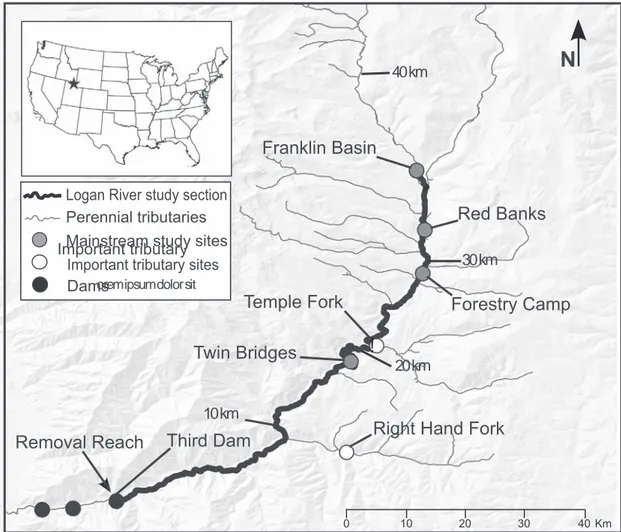
For this study, we used data from one of two primary headwater reaches (Franklin Basin) and four mainstem reaches (Red Banks, Forestry Camp, Twin Bridges, and Third Dam; Third Dam is the most upstream barrier in the river) and our sites span the range of most physical and biological conditions in the Logan River(Fig. 1; Table 1). Abiotic site characteristics are summarized in De La Hoz Franco and Budy (2005). We collected fish once a year in 2001–2016, during base-flow conditions (approximately 2.8 m3.s−1_{; conducted annually}

be-tween 15 July and 10 August) using a three-pass, electrofishing de-pletion technique with block nets at the lower and upper ends of each sampling reach. We counted all captured fish by pass and used a de-pletion model in Program MARK (Huggins, 1989) to estimate fish densities for each sample reach and each species (White and Burnham,

1999). No density estimates were possible in 2011 at three sample reaches (Franklin Basin, Forestry Camp, and Twin Bridges) due to high river flows which make sampling impossible. Monitoring surveys in 2009–2011 were conducted before (2009), during (2010), and after (2011) the mechanical removals at the Third dam reach.

2.1.5. System under study

In this study, we include the section of the Logan River mainstem spanned by the 5 sampled sites (Fig. 1), thus covering a wide range of

Third Dam

Right Hand Fork

Twin Bridges

Temple Fork

Forestry Camp

Franklin Basin

Red Banks

Removal Reach

0 10 20 30 40 Km

orem ipsum dolor sit

Important tributary

10 km

20 km

30 km

40 km

!

Logan River study section

Perennial tributaries

Mainstream study sites

Important tributary sites

N

Dams

Fig. 1. Section of the Logan River in northern Utah, USA, considered in this study. The section of the Logan River which is considered in this study (thick line) includes the mainstem river which is upstream the most upstream barrier in the river (Third dam reach; 0 km; dams are represented as black dots) up to one of two primary headwater reaches (Franklin Basin; 35.4 km). The river is characterized as high quality, connected habitat (Mohn, 2016). Five reaches have been sampled in 2001–2016 (Third Dam, Twin Bridges, Forestry Camp, Red Banks, Franklin Basin; grey dots). Some 3855 age-1 and older brown trout were mechanically removed from the lower river in 2009–2011. Two tributaries were sampled in 2001–2016 (white dots) as part of a larger study.

Table 1

Study reach features. Study reaches are located along 35.4 km of the mainstem river (Fig. 1) over a 514 m elevation range. River width (mean) and coin-cidental habitat space decrease in the upstream direction. Detailed abiotic and biotic characteristics of each site can be found inDe La Hoz Franco and Budy (2005). Location name Elevation (m) River width (m) Sampled length (m) Distance to Third Dam (km) Franklin Basin 2023 8.6 103.7 ± 9.7 35.4 Red Banks 1923 11.3 186.9 ± 21.2 30.9 Forestry Camp 1855 12.2 200.0 ± 0.0 27.9 Twin Bridges 1691 12.1 203.4 ± 29.5 17.2 Third Dam 1509 13.6 203.0 ± 14.6 0

physical and biological conditions and no barriers to fish movement. Although there are other fishes present in the fish community, their densities are extremely low relative to cutthroat trout and brown trout. Consequently, for statistical/modeling purposes herein, we believe it is fair to ignore the other fish species. We also excluded age-0 cutthroat trout and brown trout from the analysis. In the IMW cutthroat trout are spring spawners and are too small in summer to sample effectively such that densities of age 0+ are dramatically underestimated. Moreover, age-1 and older trout densities are more robust indicators of population status, especially in high-gradient, high-velocity, highly-productive habitat like the Logan River where age-0 and age 1 survival of trout in mountain streams is extremely low (usually < 10 %), variable, and hard to estimate because small fish are rarely captured with electro-fishing (e.g.,Hilderbrand, 2003). We thus aggregated age-1 and older trout densities (≥ 100 mm TL) together (simply referred to as ‘observed densities' in the following), which provides an index of subadult and adult densities. Cutthroat trout and brown trout densities observed at the 5 sites for the full period are illustrated as Appendix S1. Bilinear interpolation of these values provide a better view of the spatio-tem-poral variation of trout densities (interactive 3D plot;http://www.usu. edu/fel/laplanchetrout).

2.2. Preliminary statistical analyses

The time period covered by sampling is split in two (2001–2009 and 2010–2016) in order to investigate the effect on trout populations of the mechanical removal which took place in 2009–2011.

2.2.1. Before the mechanical removal (2001–2009)

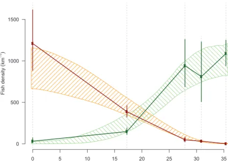
Aggregated density data prior to the mechanical removal are illu-strated inFig. 2. Brown trout have largely displaced cutthroat trout in upstream sections (as described inDe La Hoz Franco and Budy, 2005; Budy et al., 2008). Brown trout are dominant downstream (96.9 ± 1.6 % of the total), and progressively decline to complete absence upstream (0.0 ± 0.0 %). Deviations of density to the locality mean are log-nor-mally distributed (Shapiro-Wilk test after the removal of 6 outliers; p = 0.12): this property will be used later in the modeling process. Notably, density deviations are proportional to densities and are the greatest for high densities, as illustrated inFig. 2. Density profiles along the river have changed little across the 2001–2009 period (ANOVA partition of sum of squares of log-densities; spatial effect: 90.2%;

temporal: 2.5%; spatio-temporal: 7.3%). The resulting location of the inflection point for species dominance (x = 19.7 ± 1.7 km; intersection of linearly interpolated observed densities) is consequently fairly stable (p = 0.07; linear regression). Therefore, we assumed that the ecological system reached a steady state prior to the mechanical removal.

2.2.2. Response to the mechanical removal (2010–2016)

Brown trout are still completely absent upstream in 2010–2016 (0.0 ± 0.0 %, see Appendix S1). In addition, the dominance of brown trout downstream is less severe following the mechanical removal (74.9 ± 15.1 % of the total at Third Dam reach; only 51.8% in 2014; see Appendix S1), whereas cutthroat trout density reached its maximum density at the Third Dam reach (0.464 km−1_{) in 2014, after removal.}

Temporal variation in density at the Third Dam reach (algebraic dif-ferences between two subsequent years) is log-normally distributed (p = 0.58). From this statistical property, we observed that both the decline in brown trout density (2011 → 2012; p = 0.013) and the in-crease in cutthroat trout density (2012 → 2013 → 2014; p = 0.00039) following the mechanical removal, due purely to chance, are highly unlikely. While immigration into the removal reach and high natural variability in fish densities lessened the response to mechanical re-moval, based on the large number of fish removed and our under-standing of species interactions in this system, it is safe to conclude that the large-scale mechanical removal caused a decline in the density of the exotic species. This decline in the exotic species then lead to an increase in the density of the native species (Saunders et al., 2014). Somewhat unsurprisingly, there was no visible effect of the mechanical removal on trout populations at upstream reaches (17.2 km upstream Third Dam reach or further; see Appendix S1).

2.3. Modeling

2.3.1. Mathematical model

Time (in years) is denoted t. Let x ∈ (0,xup_{) denote the location along}

the river mainstem (curvilinear distance in km from Third Dam study reach; positive upstream; x = xup_{= 35.4 at Franklin Basin). Densities of}

age-1 and older trout of the exotic (here brown trout) and native (cutthroat trout) species in the river channel are denoted by E(x,t) and N(x,t) (km−1_{). Spatio-temporal variation in densities along the river}

mainstem are modeled with a 1-D, PDE-based model, using the Fisher reaction-diffusion equation with competition (Okubo et al., 1989;

Location along the mainstem (km)

Fish density ( km − 1) 0 5 10 15 20 25 30 35 0 500 1000 1500

Fig. 2. Observed and modeled trout densities at steady state. The mean (dots) of 2001–2009 density data of the exotic (dark red) and the native (dark green) species are estimated at the 5 sampling sites, which are located along the river mainstem (dotted lines); 95% confidence intervals of the observed mean (vertical thick lines) illustrate inter-annual variation, which are log-normally distributed, and conse-quently high at high density and low at low density. The 95% confidence interval of the densities which were issued in the steady state model are superimposed on the plot (polygons with shading lines). Prior to the management action of re-moval, the exotic species was dominant downstream and is progressively less dense to absent upstream.

Andow et al., 1990; Holmes et al., 1994): ⎧ ⎨⎩ ∂ ∂ = ∂ ∂ + − + − ∂ ∂ = ∂ ∂ + − + E t D E x r E E N α K x R x t N t D N x r N N E α K x / / (1 ( / )/ ( )) ( , ) / / (1 ( / )/ ( )) , E E N E N N E N 2 2 2 2 ₍₁₎

which models fish displacement (DEand DNare diffusion coefficients in

km.year−1_{), logistic growth (r}

E and rN are intrinsic growth rates in

year−1_{; K}

E(x) and KN(x) are carrying capacities in km−1), and

com-petition (αNand αEare competition coefficients; dimensionless).

Com-petition coefficients represent the relative amount of habitat of one species lost due to the presence of the other (the smaller the more competitive). Growth and competition terms aggregate different pro-cesses, including the indirect effects of limited resources/space on growth and size (e.g.,Hilderbrand, 2003; Leeseberg and Keeley, 2014), territoriality (reviewed in McHugh and Budy, 2006), and the direct effects of inter-specific competition, which can be environmentally mediated (Fausch and White, 1981; McHugh and Budy, 2005; McHugh and Budy, 2006; Öhlund et al., 2008; Korsu et al., 2009).

The PDE model further requires boundary conditions to be fully specified (plus initialization, see Appendix). Our choices of boundary conditions ascertain the observed complete absence of the exotic spe-cies at the upstream boundary (E(xup_{,t) = 0 and N(x}up_{,t) = K}

N(xup) for

all t) with no flux from/to upstream (∂E/∂x(xup_{,t) = ∂N/∂x(x}up_{,t) = 0),}

thus avoiding the specification of values at the downstream boundary where the mechanical removal took place. We additionally consider unequal carrying capacities, which are modeled as linear as a first ap-proximation ⎧ ⎨⎩ = + − = + − K x K K K x x K x K K K x x ( ) ( ) / ( ) ( ) / , E Edown E up Edown up N Ndown Nup Ndown up (2)

Where KEdown, KEup, KNdownandKNupdenote the carrying capacities in km−1

of the exotic/native species downstream (for x = 0) and upstream (x = xup_{). In order to model possible inhospitability of the}

up-/down-stream portion of the river, we allow for negative values for KEdown, KEup,

KNdownandKN

up_{, in that case, K}

E(x) and KN(x) are forced to zero when

negative. We also consider in the dynamical model the large-scale re-moval of the exotic species via the term R(x,t) (km−1_.year−1_{). Most}

processes which are relevant to the population dynamics and basic autoecology of both species, as well as their interactions, are considered by this simple model; however, there are other important complexities not considered but discussed later.

2.3.2. Steady state reached before the mechanical removal

The state of a reaction-diffusion model can, depending on the model, converge to a steady-state, which describes the constant state which is approached asymptotically by the system. The situation where the steady state would be reached before the mechanical removal oc-curred is mathematically defined as the values of E and N such that ∂E/ ∂_{t = ∂N/∂t = 0 (and in that case R(x,t) = 0). It is difficult to} analyti-cally track system steady state from latter equations, while it is rela-tively easy with numerical methods (see the Appendix). The model as such is over-parametrized for a steady state study, however. For that reason, growth parameters are reconfigured as

⎧ ⎨⎩ = = r ρ D r ρ D , E E E N N N ₍₃₎

thus making it explicit that multiplying Eq. (1) by some constant (now DEand DN) leads to the same steady state. Theoretically, it is possible to

calibrate model parameters ρE, ρN, αE, αN, KEdown, KNdown, KE up_{, and}

KN up_by

using adequate data on system steady state. We used aggregated data which were illustrated in Fig. 2 for that purpose. Calibration was achieved using a Monte Carlo Markov chain (MCMC) method. MCMC methods simulate parameter samples according to their posterior dis-tribution, requiring a model for observation errors and some prior distribution for parameters. Observation errors are modeled as

log-normal (see earlier Section 2.2) and we used flat priors for model parameters (see the Appendix). We chose to perform calibration via Bayesian MCMC methods for several reasons. First, MCMC methods are numerically efficient, in comparison to standard Newton-like optimi-zation techniques (e.g., Levenberg-Marquardt), to calibrate non-linear models of moderate complexity that are possibly over-parametrized. Second, Bayesian methods transcribe observation errors into parameter uncertainties under the form of a distribution, called the joint posterior distribution of model parameters, which basically represents the plau-sibility of each parameter combination given the data. Third, such a distribution is used later to compute the probability of eradication of the exotic species, still in a Bayesian framework. Finally, point esti-mates which are issued by Bayesian MCMC methods are very close to those which would theoretically be obtained by standard calibration methods (e.g., maximum posterior estimates using flat priors and nor-mally distributed errors are equal to Minimum Mean Square Error (MMSE) estimates).

2.3.3. Dynamical response to the mechanical removal

The dynamical response to the mechanical removal can be simu-lated by running the dynamical model starting from its 2009’s state and activating the removal term. Since we have hypothesized the system was in a steady state in 2001–2009, simulations started from the steady state found at the previous step. The number of fish which are removed from the simulated system (via R(x,t)) were those that were removed in the field (reported inSection 2.1.3). Once again, it is difficult to ana-lytically tract system state from Eq. (1) while it is relatively easy with numerical methods (see the Appendix). Simulating the dynamical re-sponse to the mechanical removal requires further calibration (DEand

DN). Calibrating these parameter cannot be achieved from steady state

(seeSection 2.3.2) which requires time series data with a deviation of the system from the steady state. MMSE estimates for DEand DNwere

computed by using time series data at the Third Dam reach with a standard optimization procedure (see Appendix S3).

2.3.4. Steady state reached after the mechanical removal and probability of eradication

The system described by Eq. (1) can also converge to a steady-state after simulating the mechanical removal (R(x,t) > 0). Depending on the values of model parameters, however (see laterSection 3.2), the system can either return to its original steady state or reach a new steady state where the exotic species is eradicated.

The probability of eradication is defined as the chance that the exotic species would, in the end, be eradicated from the system fol-lowing the mechanical removal. In a deterministic framework, with hypothetical infinite knowledge on system mechanics and system state, such a probability would be either 0 (eradication will not happen) or 1 (eradication will happen). In a framework with limited knowledge, the probability of eradication lies between 0 and 1 and is predicted con-ditionally on the current knowledge of the system available at the time the prediction is made. A portion of the knowledge on system me-chanics was transcribed into model equations (remaining knowledge on system mechanics, e.g., based on other experiments conducted in the Logan river, is used later to discuss the results). By performing model calibration in a Bayesian framework, the knowledge on system state originating from 2001–2009 data was transcribed into the posterior distribution of model parameters. The probability of eradication using data up to 2009 (denoted πerad_{) can thus be computed by exploring}

parameter space and calculating the proportion of parameter combi-nations (weighed by their posterior density) that in the end lead to eradication. Since parameter samples which were simulated by the MCMC method are distributed according to their posterior distribution, exploring parameter space is simply achieved by looping over MCMC samples, and the probability of eradication is found by numbering the cases that in the end lead to eradication.

data that were collected after 2009. The absence of a response of the native species to the significant removal would, for example, indicate the removal was inefficient. On the other hand, some increase in the density of the native species would lead to a more optimistic update of πerad. The information which is contained in the data collected after 2009 could be included in a full Bayesian framework, which will be discussed later. We limit our presentation to a single approximated update of πerad_{in 2014, by numbering the cases (via MCMC samples)}

that lead to eradication after excluding parameter samples which lead to a density of the native species at the Third Dam reach which is lower that the maximum observed value (0.464 km−1_{). Finally, the success of}

the management action likely depends on how the management action was conducted. We limit our model presentation by updating πerad_in

the cases where twice or three times as many fish were removed from the system in 2009–2011.

3. Results of the modeling

3.1. Steady state reached before the mechanical removal

Steady state, as simulated by the model, favorably compares with observations and demonstrates a progressive shift from an exotic- to a native-dominated system in the upstream direction (Fig. 2). The com-parison of prior and marginal posterior distributions illustrate how in-formative the monitoring data are with respect to model parameters (Fig. 3) and general system understanding. These data contain scarce information for calibrating the competition coefficient (αN) and the

downstream carrying capacity (KNdown) of the native species; but are

quite informative for the rest. This problem was expected due to the necessary use of 10 data points (Fig. 2) to estimate 6 parameters, which causes collinearity between model parameters, as illustrated in Ap-pendix S2. The comparison of competition coefficients between species indicate that the exotic species effectively prevents the native species from reaching its carrying capacity when present ( ̂ =αE 0.2) while the presence of the native species has a low impact on the presence of the exotic species ( ̂ =αN 3.3). Upstream habitat is more favorable to the native species (KN =1019 up l km−1_{; K} = −₂₂₃ E up l km−1_{). Downstream}

habitat is favorable for both species (KN =2070

down

l km−1_;K =₁₁₈₃ E

down

l

km−1_{). Consequently, the observed switch in species dominance along}

the river mainstem is explained by both species having some location-specific superiority over the other, more location-specifically (1) habitat avail-ability for the native species, and (2) competitive superiority for the exotic species. The native species has a constant advantage upstream (via habitat), while the superiority of the exotic species (via competi-tion) is only influential when the species is dominant, which occurs in

0.0 0.1 0.2 0.3 0.4 0.5 0 2 4 6 8 10 12 ρN PDF 0.0 0.1 0.2 0.3 0.4 0.5 0 5 10 15 20 25 ρE PDF 0 1 2 3 4 5 0.0 0.1 0.2 0.3 0.4 αN 0 1 2 3 4 5 0.0 0.5 1.0 1.5 2.0 2.5 3.0 αE 0 1 2 3 4 5 0.00 0.05 0.10 0.15 0.20 0.25 0.30 0.35 K_Ndown 0 1 2 3 4 5 0.0 0.5 1.0 1.5 KEdown −2 −1 0 1 2 0.0 0.5 1.0 1.5 2.0 KN up −2 −1 0 1 2 0.0 0.5 1.0 1.5 2.0 KEup

Fig. 3. Estimated values of model parameters. The prior distribution of model parameters (marginal priors in green) update into a posterior distribution (estimated marginal posteriors in black) via calibration in a Bayesian framework. Monitoring data are informative when both distributions differ from each other. Data are poorly informative with respect to αNand KNdown, yet are quite informative for the other parameters. Point estimates of model parameters, which are reported in the

text, are highlighted (vertical dashed black lines). Priors are uniform distributions except for ρN(see Appendix). The marginal posterior distributions and point estimates of model parameters leading to the eradication of the exotic species subsequent to the mechanical removal are superimposed to the plots (in red).

2005

2010

2015

2020

0

200

400

600

800

1000

Time (year)

Fish

density

(

km

)

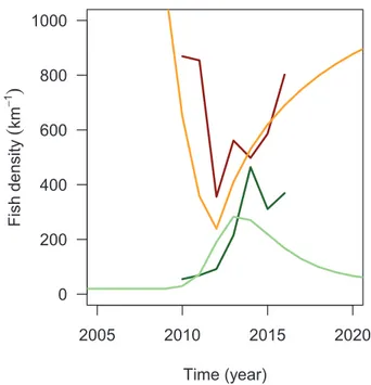
Fig. 4. System response to the mechanical removal at the Third Dam reach. The system responded to the 2009–2011 mechanical removal as a drop of brown trout density (observed densities in 2009–2016 in dark red) and a sub-sequent increase of cutthroat trout density (dark green). Such a response of the system to the mechanical removal behavior is also simulated by the model (here using point parameter estimates for model parameters; cutthroat trout: light green; brown trout: orange).

downstream sections. Carrying capacities, estimated by calibrating the model, decrease in the upstream direction for both species (KN <K up N down l l andKE <K up E down l l ).

3.2. Dynamical response to the mechanical removal

Estimated values for diffusion coefficients are DlN=0.030 and =

DlE 0.0025 km.year−1 (Appendix S3) indicating higher movement capability of the native species (DN> DE). The model effectively

re-creates the observed decrease in the exotic species as well as the in-crease in the native species following the mechanical removal (Fig. 4). The response as simulated by the model depends on parameter values, however. The increase in the native species following the mechanical removal is predicted to occur only if ρN> ρE(there were absolutely no

case among MCMC samples of an increase in the native species other-wise; not shown). As a result, we find that higher growth rates is also required by the native species (rN> rE; by using Eq. (3)) in order to

respond to the mechanical removal and demonstrate a substantial in-crease in density.

3.3. Steady state reached after the mechanical removal and probability of eradication

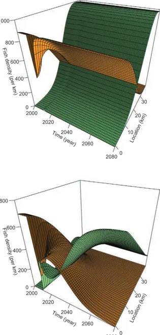
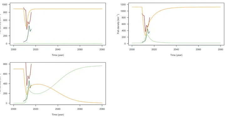
The steady state as simulated by the model following the large-scale removal also depends on parameter values. The steady state is either recovery (returning to original steady state) or eradication (reaching a new steady state) of the exotic species from the system, as illustrated in

Fig. 5. The study of the parameter posterior distribution demonstrates eradication is more likely if the exotic species exhibits slower growth (ρEis low;Fig. 3; see also Appendix S2). Depending on parameter

va-lues, the simulated response of the system at the Third Dam reach ranges from (1) no/little response of cutthroat trout to the mechanical removal, (2) a stronger response which goes back to the original state, and (3) a response which eventually leads to brown trout eradication (Fig. 5). In the latter case, the fast decrease of brown trout density at the Third Dam reach subsequent to the mechanical removal is followed by a slow increase and a decrease again this time to eradication (seeFig. 6). The rapid increase in cutthroat trout density is on the other hand fol-lowed by a slow decrease and an increase again to the full reoccupation of the niche. In view of these modeling results, the increase of brown trout density and the decrease of cutthroat trout density that are pre-sently (2014–2016) observed at the Third Dam reach thus could either indicate the failure or the success of the management action.

The probability that brown trout would be eradicated from the system using 2001–2009 data is low (0.7 %; see Table 2). Such a probability, however, increases to 21.3 % if 3 times as many brown trout are theoretically removed at the Third Dam reach. Using 2010–2016 data, due to the observed increase of native trout density in 2010-2014, the probability that brown trout would be eradicated raises to 20.5%. Such a probability increases further to 68.9% if 3 times as many brown trout are theoretically removed at the Third Dam reach.

4. Discussion

As a summary, we have presented an interactive spatially explicit 1D, 2-species/2-state variable, reaction-diffusion model with constant diffusion, logistic growth, linear carrying capacities, and first-order competition rates. The model is relatively simple, yet it results in a realistic simulation of the system under study (seeSection 4.1). Iden-tifying and discussing key model assumptions (seeSection 4.2) helps us make suggestions of potential model and data improvements. We close with a review of the use of this type of models to guide management efforts aimed at eradicating exotic fish species from riverine ecosystems or some other similar management action (seeSection 4.3).

4.1. Realistic simulations of system state

Our model captures the shift of species dominance along the river mainstem (Fig. 2) and the dynamic response to the mechanical removal (Fig. 4); both fit long-term monitoring data. The allopatric distribution of species along the Logan River has been well established (e.g.,

McHugh and Budy, 2005) and is nearly perfectly captured by our in-dependent modeling results. Similarly, we observed a large decline in brown trout abundance immediately after mechanical removal, in-dicating these model predictions also accurately capture what was ob-served in nature (e.g.,Saunders et al., 2014).

Our framework also led us to estimate key parameters (diffusion coefficients, carrying capacities, growth rates, competition coeffi-cients), and these relative values (between species; upstream v. down-stream in the case of carrying capacities) are consistent with available knowledge. Notably, empirical knowledge was not used for parameter calibration (parameters were provided with vague flat priors) and is used here only to measure the consistency of our results.

More specifically, we observed carrying capacities decrease in the upstream direction (KE <K

up

Edown andKNup<KNdown). Carrying capacity

likely changes as a function of habitat availability, which in turn changes somewhat in a longitudinal pattern due to the natural, geo-morphic reduction in river width and coincidental habitat space available (Mohn, 2016). Considerable variation in environmental and stream conditions occurs along the longitudinal and elevational gra-dient of the Logan River, due to changing geology and hydraulics, which influence native and exotic trout densities (Budy et al., 2008; Meredith et al., 2015). Like others, we observed that the upstream river was inhospitable for brown trout contrary to cutthroat trout (KE ≪K

up N up

). In contrast to most native fishes in the IMW, which spawn in the spring (April to June), brown trout are autumn spawners (Oc-tober to December). Headwater reaches of the Logan river experience localized anchor ice freezing in winter (January to March), offering one potential mechanism whereby upstream sections are inhospitable for spawning and larval brown trout (Meredith et al., 2017). This ob-servation may explain why brown trout spawning is relegated to available gravel in more downstream sections of the river network (Wood and Budy, 2009; Meredith et al., 2017).

We also observed that the predicted presence of brown trout se-verely hinders the performance and growth of cutthroat trout, while brown trout were unaffected by the presence of native cutthroat trout (αE< αN). In smaller, controlled experiments and larger reach-scale

experiments, brown trout similarly reduced the growth, altered the diet, and suppressed the movement of native trout (seeMcHugh and Budy (2005), Saunders and Budy (in revision)). We have observed little evidence of brown trout predation on cutthroat trout in this system, however (Meredith et al., 2015). At the same time, likely because they are competing for space and dominating the preferred territories, brown trout are unaffected by the presence of native cutthroat trout (McHugh and Budy, 2005). Brown trout often display a strong ag-gressive behavior compared to other salmonids (Fausch and White, 1981). Moreover, the aforementioned earlier spawning of brown trout may give exotic brown trout a temporal advantage over native cut-throat trout, thus giving age-0 brown trout a strong size advantage over native cutthroat trout in the summer (June to September), a critical time period for growth. This size advantage could intensify competitive interactions, particularly aggressive behavior and competition for space (e.g.,Budy and Gaeta, 2017), giving brown trout an even greater ad-vantage overall.

Finally, we observed cuthroat trout displaying higher predicted movement (DE> DN) than brown trout. Exotic brown trout are

wide-spread and abundant because they are vagile (capable of dispersal) and have a large fundamental niche (Mcintosh et al., 2011; Budy and Gaeta, 2017). Both species of trout have the capacity to exhibit substantial growth rates in the Logan River (Budy et al., 2007, 2008). However, cutthroat trout also have the potential to move great distances (e.g.,

Hilderbrand and Kershner (2000); whereas brown trout are more often sedentary and show high rates of site fidelity in this system, e.g.,Budy et al., 2008).

We predicted that despite the large effort to remove brown trout mechanically (> 4100 fish removed), the probability of complete era-dication is low in the mainstem based on mechanical removal. We observed little modeled effect of the mechanical removal at reaches upstream of the Third dam reach (see Appendix S1), and the predicted probability of eradication was low using data pre-2009 (0.7%). These predictions concur with what has been observed elsewhere (reviewed in

Saunders et al., 2014; Budy and Gaeta, 2017), often leading managers to resort to chemical treatment where feasible. However, using more recent data, the predicted probability of eradication increases con-siderably (20.5%). Presumably this increase is in response to the ob-served increase in the density of cutthroat trout at Third Dam, likely in

turn in response to the decrease in the superior competitor, brown trout. In other work, we have demonstrated it may not be necessary to completely eradicate the invasive fish, if the density advantage can be switched back to the native fish, allowing ‘biotic resistance’ to operate (Saunders and Budy, in revision). In addition, in a nearby tributary, the densities of cutthroat trout increased dramatically to natural levels only 4 years after complete brown trout removal (P. Budy, unpublished data). Further, the propagule pressure of brown trout has declined significantly to almost zero, with the cessation of brown trout stocking. That said, brown trout are still one of the world's most invasive and destructive organisms, and environmental changes associated with cli-mate change may be more favorable to exotic trout in this region (Budy and Gaeta, 2017). As such, the suppression of brown trout in this system seems unlikely, but is still worthy of consideration given the con-servation priority of this particular population of native Bonneville

Time (y ear) 2000 2020 2040 2060 2080 Location (km) 0 10 20 30

Fish density (per km)

0 200 400 600 800 1000 Time (y ear) 2000 2020 2040 2060 2080 Location (km) 0 10 20 30

Fish density (per km)

0 200 400 600 800 1000 1200 Time (y ear) 2000 2020 2040 2060 2080 Location (km) 0 10 20 30

Fish density (per km)

0 200 400 600 800

Fig. 5. Examples of system response to the mechanical removal. Simulated densities (z-axis) for the native (green) and the exotic (orange) species are represented over time and along the river mainstem. Different scenarios can be simulated by the model, depending on parameter values: no/little response of cutthroat trout to the mechanical removal (top left), a stronger response which returns to the original state (top right), and a response which eventually leads to brown trout eradication (bottom). Parameter values in the second case are point estimates reported in the text. Densities of the native species were rescaled in the third case (K_Nup>800km−1_{) in order to superimpose native and exotic densities on the same plot. A focus on density values at the removal reach for these 3 cases is presented} inFig. 6.

cutthroat trout (the largest remaining across its range; Budy et al., 2007). Our modeling approach allows us to consider different levels of effort required and to explore targeted management at a population level.

4.2. Model/data limitations and countermeasures

Relaxing model assumptions implies refining the definition of ex-isting processes or adding new processes into the model. Both options lead to additional sets of parameters, which require specific data either for calibration or for their connection to external drivers via covariates, as explained below.

4.2.1. Incorporating age

Some of the fish attributes considered in our model are likely to vary as a function of fish age, notably between the youngest ones (age-0 individuals) and the others (age-1 and older). In the case of sedentary fish, we observe some age- or size-related variation in growth (Budy et al. 2007), dispersal rates (e.g., Gillanders et al., 2015), and/or competitive abilities (Persson, 1988); however, the latter two appear to

be rather stable amongst subadults and adults in this system (Mohn, 2016). Nevertheless, the need to apply the model to less productive rivers, and the fact that processes (e.g., growth, dispersal) are age/size-dependent, would require incorporation of age/size into the model. Fish size is readily collected in monitoring surveys, but age is difficult to estimate effectively without euthanizing fish (Laplanche et al., in re-vision). However, in stream-dwelling trout, size is a straightforward proxy to separate age-0 trout from the rest, and can demonstrate size classes highly correlated with age classes (Ruiz and Laplanche, 2010). Incorporating a size/age structure may improve simulations of some aspects of population dynamics (see for instanceGouraud et al., 2001; Sebert-Cuvillier et al., 2007; Vorpahl et al., 2009; Bret et al., 2017). However, this improvement comes at a high complexity cost due to new sets of unknown parameters (e.g., recruitment and mortality rates) re-quiring specific data for calibration. Nonetheless, incorporation of size/ age structure would allow us to refine existing processes, e.g., size/age-dependent dispersal and/or shifts in competitive dominance. This may be an area fruitful for future exploration.

4.2.2. Incorporating the river network structure

Herein we model only patterns of species density and responses to management actions in the mainstem of the Logan River; however, population dynamics and management actions in the tributaries could also influence patterns observed in the mainstem (Hansen and Budy, 2011; Hough-Snee et al., 2013). For example, in other work, we have demonstrated that a tributary (Right Hand Fork; seeFig. 1) likely acted as a source population of brown trout to the lower river (Saunders et al., 2014). When densities of exotics were high, brown trout, mostly juve-niles, likely emigrated out of the tributary into the mainstem. None-theless, density-dependent emigration of exotic brown trout operates largely on juveniles (Lobón-Cerviá and Mortensen, 2005), and the fish response observed and modeled in the lower river was for subadults and adults (Saunders et al., 2014). The mechanical removal we investigated in this paper also included removal in this tributary (Saunders et al., 2014). However, at the time of this study, management action likely had only a minor influence on this mainstem study area, if at all (i.e., there would have been a several year lag for potentially emigrated

2000 2020 2040 2060 2080 0 200 400 600 800 1000 Time (year) Fish density ( km − 1) 2000 2020 2040 2060 2080 0 200 400 600 800 1000 1200 Time (year) Fish density ( km − 1) 2000 2020 2040 2060 2080 0 200 400 600 800 Time (year) Fish density ( km − 1)

Fig. 6. Examples of system response at the removal reach to the mechanical removal. The removal reach responded to the 2009–2011 mechanical removal as a decline in brown trout density (observed densities in 2009–2016 in dark red) and a subsequent increase in cutthroat trout density (dark green). Different scenarios can be simulated by the model, depending on parameter values (see legend ofFig. 5). Densities at the removal reach as represented here (cutthroat trout: light green; brown trout: orange) were computed using the same parameter values as inFig. 5.

Table 2

Estimated probability of eradication of the exotic species. The probability of eradication (here in %) is defined as the chance the exotic species would be eradicated following the mechanical removal of brown trout that took place at the Third Dam reach in 2009–2011. Three scenarios are considered, by simu-lating the removal of the actual removed quantity (×1), or by simusimu-lating the removal of twice or three times as many fish, which illustrates the level of increase of the success of the management action as a function of its strength. Cutthroat trout density at the Third dam reach significantly increased from 2009 to 2014 (see Appendix S1), as does the chance that the mechanical re-moval would lead to brown trout eradication. The value of the probability of eradication (second row) is updated (third row) based on the observation that the density of cutthroat trout increased up to 0.464 km−1_{in 2014.}

Scenario × 1 × 2 × 3

πeradin 2009 0.7 6.6 21.3

juveniles to become adults in the removal area, Right Hand Fork). In addition, exotic brown trout that emigrated out of the tributary could just as easily migrate further upstream in the mainstem (versus down-stream into the study area). Nonetheless, evaluating the importance of tributaries on mainstem population dynamics could be possible by si-mulating our 1D model over interconnected stream sections composing the river's hydrological network. Running the model at this extended spatial scale would require either (1) more assumptions regarding whether or not stream section specific parameters are equal or similar to each other, (2) more data, across the hydrological network in order to calibrate stream section specific parameters, or (3) well-defined re-lationships between model parameters and covariates (also requiring data for calibration) that could be used to predict stream section-spe-cific parameter values. This is another area fruitful for future con-sideration, but it would require acquisition of some data currently un-available even for this well studied population. In addition, Mohn (2016)found little evidence of spatial population structure in a recent complimentary mark-recapture and genetics study.

4.2.3. Incorporating covariates

Temporal variation in fish density was disregarded in this case study because spatio-temporal variation was largely of spatial nature (90.2%; seeSection 2.2). The fish community in the Logan River has remained surprisingly stable over time, and the distribution and density has de-monstrated little inter-annual variability (when not manipulated;

McHugh and Budy, 2005; Budy et al., 2007; Budy et al., 2008). Simi-larly, in its current form the model simulates ‘smooth’, spatio-temporal variation in fish density, and erratic variation is relegated to external, residual errors (see Figs. 5 and6). Sporadic, temporal variation of densities in ecological systems is the consequences of both intrinsic (e.g., density-dependent recruitment) and extrinsic (e.g., discharge-de-pendent recruitment) factors (Bischoff and Wolter, 2001; Jonzen et al., 2002; Lobón-Cerviá and Rincón, 2004). Fish intrinsic traits (in our case mobility, growth rate, competitive ability, and carrying capacity) may vary according to environmental fluctuations through time (e.g.,

Raimondo, 2012; Roy et al., 2013), which may in turn cause fluctua-tions in fish density.

Changes in carrying capacities may be important to consider when studying population dynamics and risk of extinction. In addition to simple space requirements (i.e., volume of water), the suitability of habitat (e.g., depth, velocity) and the availability of food are extremely important for trout (e.g.,Rosenfeld and Boss, 2001; Piccolo et al., 2014; Rosenfeld et al., 2014). Variation in habitat suitability along the river mainstem is thus expected to be more complicated than a simple linear function. BothMohn (2016) and Meredith et al. (2017)demonstrated that there are important local differences in habitat quantity and quality and likely suitability, that do not necessarily vary longitudinally and may also vary depending on species. Further, environmental characteristics in some systems can be highly variable through time, and may notably result in changing carrying capacity over time (Fowler and Pease, 2010). Our model could be improved with respect to habitat suitability by incorporating carrying capacities estimated from third-party models, either calibrated empirical habitat models that have a low requirement of field data (Hayes and Jowett, 1994), reach-level habitat characteristics available system-wide using a Riverstyles ap-proach (Brierley and Fryirs, 2005; Mohn, 2016), or perhaps 2D net rate energy intake models, that use external variables such as hydraulics and macro-invertebrate density and model fish movement. However, some of these approaches to estimating carrying capacity may be not ap-plicable at large scales due to considerable data and computational requirements (e.g.,Hayes et al., 2007; Urabe et al., 2010).

In our work dispersal is modeled by constant diffusion, which si-mulates the effect of a Brownian motion (random walk). The dispersion kernel – probability density function of dispersal distances at each step – is Gaussian in our case and many other options for dispersal kernels could be considered (Jongejans et al., 2008; Nathan et al., 2012).

Salmonid movement in rivers is more complex than random dispersal, however, see for instanceHayes and Thompson (2014), and mechan-istic expressions for non-random dispersal have also been modeled in an extended PDE framework (Jongejans et al., 2008; Nathan et al., 2012). Salmonid movement is often influenced by river flow (for instance, individuals may move downstream during high spring flowsYoung, 1994), which could be modeled by adding an advection term related to discharge (Hui et al., 2011). Like many animals, fishes also migrate to feeding, mating, or rearing locations, to seek out seasonal refugia, and to colonize unoccupied or under seeded habitats; these migrations are often associated with specific ages and/or seasons (Dingle, 1996; Brenkman et al., 2007). However, in this system, while a few fish moved as much as 1 km, most fish moved very little (< 100–200 m) and were located in the same reach across years (Mohn, 2016). In any cases, calibrating/comparing more advanced dispersal models would require data providing direct information on fish movement, for instance cap-ture-recapture data (Marvin, 2012).

4.2.4. Incorporating a dynamic system

In its current form, the model actually simulates (not shown) that the downstream introduction of the exotic species creates a wave of dominance of the exotic species, which travels in the upstream direc-tion and stops (steady state) at a stable point at a given locadirec-tion in the river. Such an inflection point is the consequence of both species having some competitive superiority over the other, with dominance of the native species upstream. Native fishes are often relegated to the head-waters, where they may have a slight competitive advantage due to abiotic conditions (reviewed inBudy and Gaeta, 2017) although the reverse could occur (e.g.,Cucherousset et al., 2007). Exotic fish can also drive native species to extinction (reviewed inBenhke, 1992, Hasegawa et al., 2014). In that case, the wave of dominance does not stop at a stable point at a given location in the river. Our model can actually simulate invasion towards the point of extinction of the native species, by specifying appropriate boundary conditions (e.g., time-dependent decreasing density of the native species upstream). Model calibration for systems in which a stable inflection of species dominance hasn’t been/will never be reached could be achieved in a similar Bayesian framework, by using spatio-temporal data on a sufficiently large time period to include a significant shift in system state. In that case, all model parameters (rE, rN, DE, DN, αE, αN, KEdown, KNdown, KE

up_{, and}

KN up₎

would be estimated at the same time from the data, still using a MCMC method. The probability of eradication would be computed as we did (loop over MCMC samples) while encompassing some new features: (1) absence of a steady state, (2) uncertainties on all parameter estimates, and (3) full consideration of the data that were available at the time a forecast is made, thus extending the framework that we have presented to systems in which a stable inflection of species dominance hasn’t been/will never be reached.

4.3. Models to guide management and conservation efforts

The removal of exotic fish is often part of important conservation efforts aimed at reducing the negative impacts of exotic fishes on native fishes or other trophic levels, restoring ecosystem function, and pro-tecting economically-valuable sport fisheries (e.g.,Giles, 1994; Knapp et al., 2007; Pope, 2008). Complete eradication of exotic fish may be extremely difficult and expensive (reviewed inSaunders et al., 2014). Fishes have been successfully eradicated at small spatial scales (Syslo et al., 2013), the efficacy of fish eradication decreasing with increasing spatial scale (Britton et al., 2011). There is potential for exotic fish to be managed, controlled, or contained within large areas even if eradica-tion is unfeasible (Britton et al., 2011). However, these removal or eradication efforts are often management activities and are thus em-pirical; they rarely attempt to generate predictions or test theory.

Similar modeling approaches to the one used herein can be used to model invasion and extinction across a variety of ecological systems. An

increasing endeavour towards invasive species modelling has been observed, mostly since the 1990’s (Buchadas et al., 2017), following the same trend as for ecological modelling in general (Jørgensen, 2008). Such models have been useful to understand and forecast biological invasions. For instance,Okubo et al. (1989)used a 2D model similar to ours to predict the progress of grey squirrel invasion in the UK.Kolar and Lodge (2002), using a risk assessment approach, were able to predict the invasive potential of fish species into the North American Great Lakes from their biological traits.

From an extensive literature survey,Buchadas et al. (2017) have shown that dynamical models represented roughly one third of the modelling records focused on invasive species, and about half of these were designed for management purposes. Mechanistic, spatially-ex-plicit, dynamical models, either PDE-based such as ours or using a different mathematical framework, allow simulation of invasion of an exotic species and the reverse process following a management action. Such models thus offer insights for managers on different forecasting aspects: invasion, extinction, eradication, and recolonization. The im-portance of having spatially-explicit, dynamical models is exacerbated in view of the central role of the spatial scale and the timing (continued removal efforts) for suppression attempts to be successful. The use of dynamic modelling has been a successful way to improve our knowl-edge of population dynamics of invasive species, emphasizing the im-portance of processes such as dispersal, growth and recruitment, and relating them to Allee effects (seeBuchadas et al. (2017)for a review). Extinction risk is typically thought to be high at low densities, as small populations can be particularly affected by stochastic catastrophic events (Gravel et al., 2011). Population growth rates will typically decline or become more erratic as a population nears or exceeds car-rying capacity, and the risk of extinction is inherently higher at small population size (Morris and Doak, 2002). Moreover, the growth rate of such populations is often lowered according to Allee's principles, which further increases their risk of extinction (Gerber and Hilborn, 2001). Although Allee effects are often seen as a bane in conservation efforts, reducing exotic populations below Allee thresholds may thus be an effective strategy to eradicate invasive species (Potapov and Lewis, 2008; Tobin et al., 2011).

It is important to stress out that the probability of eradication that is computed is conditional on the knowledge available at a given time. Updating the information – data or knowledge on system mechanics – changes the distribution of model parameters (or the set of model parameters) and thus changes the estimate of the probability of eradi-cation. We have illustrated this concept by updating the value of the probability of eradication using 2010–2016 data. We discuss the fact that our model is very simple and that some aspects of population dy-namics and trout ecology were not accounted for completely. When a model is used for decision making, it should be done with caution, keeping in mind model assumptions and limitations (Burnham and Anderson, 2010). Beyond the improvement of our forecasting ability through the use of updated information, the inclusion of extra variables such as size/age or sex, or via the consideration of space or inter-sea-sonal patterns of fish activity, would potentially allow us to optimize management strategies. Some other modeling studies have shown, for instance, that the timing of harvest through the reproductive season plays an important role in the eradication success of a target species, and also that a reduction of harvest effort is possible via the optimi-zation of harvesting timing (Shyu et al., 2013; Cid et al., 2014). Model-based approaches thus have a strong potential to help allocate man-agement efforts through space and time, and target efforts to specific sex or age categories.

Overall, our study suggests that when there are high densities of the native species remaining somewhere in the system, there is hope for restoration and conservation. Our simulation exercise indicates that removal efforts for exotic brown trout should be under consideration, particularly when there are some locations in the connected watershed where high densities of native trout still occur. Every sub-species of

native cutthroat trout currently has a protected status due to dramatic reductions in abundance and distribution. Given this, it would be beneficial to consider conservation efforts that are creative and proac-tive that focus management on actions having the potential to reduce the density of exotic competitive and/or predatory fishes.

Acknowledgments

The data collection component of this study was funded by the Utah Division of Wildlife Resources and the U.S. Forest Service, Rocky Mountain Research Station. The U.S. Geological Survey Utah Cooperative Fish and Wildlife Research Unit (in-kind) and the Ecology Center at Utah State University provided additional support. The au-thors acknowledge INPT’s financial support, which contributed to the initiation of this project. We would like to thank the numerous field technicians and volunteers who helped in data collection. We are grateful to Brett Roper (USFS, RMRS) who has been involved in many aspects of this broader study, and he provided many helpful comments along the way. Pete McHugh reviewed earlier drafts of this manuscript and provided helpful comments. We performed this research under the auspices of Utah State University IACUC Protocol 2022. Any use of trade, firm or product names is for descriptive purposes only and does not imply endorsement by the U.S. Government.

Appendix A. Numerical computations A.1. Solving PDEs

PDEs were numerically integrated by being converted to ordinary differential equations by numerical differentiation before numerical solving. Numerical integration used a 1-km spatial unit and 1-year time step, both were sufficient (results remained unchanged at higher spatio-temporal resolutions). Interpolated monitoring data (Fig. 2) were used for initialization. Steady state was found either using a Newton-Raphson method (fast) or, when this failed, by dynamically running to steady state (slower). PDE computations were carried out with R ver-sion 3.4 using packages rootSolve, FME, and deSolve.

A.2. MCMC simulation

MCMC samples were simulated using Metropolis-Hastings algorithm (300,000 it.; 8 chains). MCMC jumps were adjusted by using the parameter covariance matrix as resulting from fitting the model with the adaptive Metropolis-Hastings algorithm (20,000 it.). Parameters were assigned flat priors with the following boundaries which were deemed sufficient by avoiding parameter clipping: ρN∈(0,0.5), ρE∈

(0,0.5), αN ∈ (0,5), αE ∈ (0,5), KNdown∈(0, 5), KNup∈(0, 5),

∈

KEdown (0, 5), andKEup∈ −( 5, 5). Given that the observed increase in

the native species never happened if ρN< ρE, the MCMC method was

run again by forcing ρN> ρE, in that case ρN− ρE∈(0,0.5) was simu-lated instead of ρN. The resulting marginal prior distribution for ρNis

triangular. Parameter priors are represented inFig. 3. MCMC compu-tations were carried out with R version 3.4 using packages FME and doMC.

Appendix B. Supporting information

Additional Supporting Information may be found in the online version of this article at https://doi.org/10.1016/j.biocon.2018.04. 024.

References

Abrams, P.A., 2009. When does greater mortality increase population size? The long history and diverse mechanisms underlying the hydra effect. Ecol. Lett. 12, 462–474.