Any correspondence concerning this service should be sent
to the repository administrator:
[email protected]
This is an author’s version published in:
http://oatao.univ-toulouse.fr/n° de post 19081
To cite this version:
Arenas, Helbert and Islam, Md Bayzidul
and Mothe, Josiane Overview of the ImageCLEF 2017 Population
Estimation (Remote) Task. (2017) In: International Conference of
the CLEF Association, CLEF 2017 Labs Working Notes (CLEF
2017)), 11 September 2017 - 14 September 2017 (Dublin, Ireland).
Official URL: http://ceur-ws.org/Vol-1866/invited_paper_2.pdf
Open Archive Toulouse Archive Ouverte
OATAO is an open access repository that collects the work of Toulouse
researchers and makes it freely available over the web where possible
Overview of the ImageCLEF 2017 Population
Estimation (Remote) Task
Helbert Arenas(1), Md Bayzidul Islam(2), Josiane Mothe(1)
(1) IRIT, UMR5505, CNRS & Universit´e de Toulouse, Toulouse, France (2) Institute of Geodesy, Faculty of Civil and Environmental Engineering, Technical
University of Darmstadt, Germany
Abstract. Estimating population has many applications as planning disaster responses, communication infrastructure, or development activ-ities. In 2017, ImageCLEF Lab introduced a new pilot task: the Popula-tion EstimaPopula-tion (or Remote) task which aims at estimating the popula-tion of an area of interest by exploring Copernicus earth observapopula-tion data (i.e. free Sentinel-2 satellite images). In line with the goal of FabSpace 2.0 project, a European Unions initiative to bring Geo-Enthusiast together around the 6 European universities in collaboration with Business Incu-bation Centers, participated to this challenge. This paper presents the results that were obtained by the participants as well as a brief summary of some of the approaches that were used.
Keywords: Information Systems, Information Retrieval, Image Retrieval, Coper-nicus data, Automatic Population Estimation, FabSpace 2.0, CLEF
1
Introduction
Estimating population for the planning of communication infrastructure and any development activities is an important issue. Such accurate estimation is also crucial for NGOs before engaging any rescue operation or humanitarian action. Population estimation is indeed fundamental to provide any services for a particular region. While good estimates exist in many parts of the world through accurate census data, this is usually not the case in developing countries. Collecting new census is expansive and time consuming; it is not possible in case where decision has to be taken quickly. Moreover, census data are generally based on political areas such as cities or counties while humanitarian and rescue actions and/or communication activities are more geographically-based as they take place in the areas of catastrophe such as where hurricane, earthquake or flood happened and to combat epidemic diseases.
Alternatively, counting the number of buildings (given the fact they can be properly extracted) can provide a first estimate; however, it may not be enough since people in various places in the globe do not live the same way, the population may vary in summer and winter in different touristic places, or population may vary where there is easy access to public services or amenities.
Moreover, the distribution of population in the coast and the urbanized area is not similar in terms of building structures and spatial distributions, household sizes and topographical representations.
This pilot task is part of the imageCLEF 2017 Labs [13] and was introduced this year. It aims at investigating the use of non commercial satellite data as a free and quicker process to estimate the population of an area of interest. More specifically, this pilot task aims at exploring Copernicus1arth observation
data (i.e. Sentinel-2 satellite images) which are available for free and in a good temporal and spatial resolution.
2
Population Estimation Pilot Task Overview
In this pilot task, participants had to estimate the population for different areas in two regions Lusaka and Uganda. To achieve this goal, organizers provided a set of satellite images (Copernicus Sentinel-2). The boundaries of the areas of interest were provided as shape files. The clipped satellite images were provided as well as the meta data of the original images (before clipping). This pilot task uses Copernicus Sentinel-2 multi-spectral images with 13 bands (resolution between 10 and 60 meters). However, participants were allowed to use any other resource they think may help to reach the highest accuracy.
The study area consist of 83 areas of interest in the city of Lusaka and 17 in west Uganda for which the population has to be estimated, for a total of 100 areas. For 90 of these areas ground truth is available thus evaluation considered these areas only.
This pilot task was initiated within FabSpace 2.0 project2 in collaboration
with CartONG, founded in 2006, CartONG is a French non-governmental or-ganization committed to furthering the use of geographic information tools to improve data gathering and analysis for emergency relief and development pro-grammes around the world.3 The task is an open challenge in the ImageCLEF
laboratory as well as in the 6 FabSpaces laboratory in Europe.
3
Dataset and evaluation protocol
3.1 DatasetThe data set4 consists of topographic and geographic information as follows:
1
www.copernicus.eu/main/sentinels
2
FabSpace 2.0 is the open-innovation network for geodata-driven innovation by lever-aging Space data in particular, in Universities 2.0. This project received funding from the European Unions Horizon 2020 Research and Innovation program under the Grant Agreement no
693210. More information at https://www.fabspace.eu/ and [6]
3
http://www.cartong.org/fr
4
The dataset is available on Zenodo with the DOI 10.5281/zenodo.804602 or on de-mand
– ESRI shape files: there is single shape file by region and the projected shape file of the region has the necessary attributes to represent the various areas the region is composed of.
– Sentinel-2 satellite images: The remote sensing imagery comes from the Sentinel-2 platform. The imagery is multi spectral, cloud-free satellite im-agery downloaded from Sentinel Data Hub5. The images have been clipped to
match the bounding box of the areas of interest. The bands for images have different spatial resolutions: 10 meters for bands B2 (490nm), B3 (560nm) B4 (665 nm) and B8 (84nm); 20 meters for bands B5 (705nm), B6 (749nm) B7 (783nm), B8a (865nm) B11 (1610nm) and B12 (2190nm). For the anal-ysis, participants were encouraged to use Red, Green and Blue bands or in some cases near infrared bands which are 10 meters resolution.
– Meta-data associated to the images: Information regarding the original im-ages is provided in XML files. These files contain information like capture time/date, sensor mode, orbit number, the id of quality files, etc. Further information regarding the Sentinel-2 products, as well as file structure can be found in the Sentinel 2 User handbook6.
In this pilot task two regions has been selected: city of Lusaka and West of Uganda. More specifically, the data set is composed of the following structure:
– City of Lusaka: The subareas are based on Operational Divisions, a unit defined by M´edecins Sans Fronti`eres in 2016. This organization divided the city of Lusaka in 83 units. For this region, the data set consists of: (1) ESRI shape file including locational and attributes information, (2) Two Sentinel-2 level-1C satellite images covering the area and for each image there are all 13 bands, (3) XML meta data associated to image files.
– West Uganda: In Uganda there is 17 subdivisions and for this region data sets consists of: (1) ESRI shape file including locational and attributes in-formation, (2) Five Sentinel 2 level-1C satellite images covering the area and for each image there is all necessary bands, (3) XML meta data associated to image files.
The images from the data set are stored in zipped files with the following folder structure:
5
https://scihub.copernicus.eu/dhus/#/home
6
[NAME OF THE STUDY REGION]: Lusaka or Uganda.
[shp]: This folder contains a shapefile with the boundaries of the study areas.
[sentinel2]
[ID OF SATELLITE IMAGE]: Original id of the image as in the Sen-tinel Data Hub.
[bands]: This folder contains the bands of the image. Each band is a Geo-Tiff file. Each band corresponds to a certain electromagnetic spectrum captured by the sensor.
[xml]: This folder contains the XML files that contains metadata in-formation regarding the images.The inin-formation applies to the original source (before image clipping). By using the information in this file a user can obtain the original dataset.
3.2 Evaluation
The evaluation method uses three metrics that compare the predicted values and the ground truth s: 1) Sum of the differences over the areas, 2) Root Mean Square Error, and 3) Pearson correlation.
The challenge comprise of geographically separated two areas, West Uganda, and Lusaka in Zambia. Because of this fact, it was decided to evaluate both areas separately but together in a single file. We evaluate the results considering two variables: 1) Population counts, and 2) Dwelling counts. Each run submitted by the participants has 12 possible metrics. However, not all the participants sub-mitted results for both variables. All the submissions provided were estimation of the population, while only two of them provided estimates for both population and dwelling units.
The next subsections will provide a short description of the metrics used to evaluate the results.
Sum of differences This evaluation criteria estimates the differences between the predicted value and the ground truth. For each operational zone, we calculate the absolute value of this difference and summing up for the whole areas. The equation used is:
SumDelta =
n
X
t=1
|(dt− st)|
Where n represents the total number of operational zones to evaluate, dt
represents the ground truth value, and st represents the estimation produced by
the participant for the operational zone t.
Root Mean Square DeviationRoot Mean Square Error (RMSE) (also known as Root Mean Square Deviation) is one of the most widely used statistics to compute the differences between a modeled output and the observed values.
The individual differences between the produced estimation and ground truth and/or the standard deviation of residuals are called prediction errors (dt−st). If
the ground truth is dt and the estimated values is st are standardized (resulting
in zero means and unit standard deviation) then the RMSE between dt and st
can be calculated by following equation [4].
RM SE = r Pn
t=1(dt− st)2
n
The variables depicted in this equation are the same as the one previously described in the previous section for the equation Sum of differences.
Pearson Correlation this evaluation process calculates the Pearson correla-tion between the run estimates and ground truth values. Pearson correlacorrela-tion is between +1 and −1, where +1 represents absolute positive linear correlation, 0 represents no correlation, and −1 represents negative correlation [17].
r = Pn t=1(dt− d)P n t=1(st− s) q Pn t=1(dt− d)pP n t=1(st− s)
AvgRelDelta We considered an additional measure we called the average of the relative deltas which is defined as follows/
Let us consider the relative delta as (dt−st)
dt . The range of values is from
−∞ to 1. Negative values indicate overestimation, while positive values indicate underestimation.
We can then calculate the relative delta in percentage as (dt−st)
dt ∗ 100
The range of values would be −∞ to 100. This measure will be used for the maps depicting the results in the next section. We can calculate this value at the operational zone level. In this way we can indicate in which operational zone the proposed algorithm failed, how much and in which way (overestima-tion/underestimation).
However, to obtain an overall estimation for all the operational zones, it is necessary to use the absolute value of the relative deltas as |(dt−st)|
dt ∗ 100.
Otherwise, the delta values could cancel among themselves.
Then we obtain an average of the relative deltas which is defined as:
AvgRelDelta = Pn t=1 |(dt−st)| dt ∗ 100 n
where n is the number of operational zones considered for the estimation. The lower the value of AvgRelDelta the more accurate the approach is.
4
Participants and results
Although the pilot task was opened to anyone, the actual participants came from local events (i.e. Hackathon, Idea contest etc.) that were organized within
FabSpace 2.0 project in the 6 local FabSpace laboratories. Although different teams started working on the pilot task, four teams only managed to send a run (See Table 1 in the next section). Details can also be found in [2].
The methodologies and the background of the members of the participating teams was heterogeneous. For instance, in the case of Italy, the participating team was composed of two students from the university Tor Vergata, one is a Management Engineering student while the second one is a Computer Science Engineering student [18]. In the case of Greece, the background of the partic-ipants included domains such as electrical and mechanical engineering as well as business studies [15]. From Germany three participants participated where one is a graduate student of Environmental Engineering, second is a student of Physical Geography and the third one is a PHD student [14]. Also a couple of participants from diverse background were participated at Poland.
The approaches used were also diverse. In the case of Italy, the participants used an approach based on a convolutional neural network (CNN) that makes use of Sentinel-2 Imagery as well as built up estimates provided by the Cen-ter for InCen-ternational Earth Science Information Network (CIESIN) [18]. While in the case of Germany, the approach was based on supervised and unsuper-vised image classification with the inclusion of not only optical but also radar imagery [14]. The classification also includes supervised as Minimum Distance and Maximum Likelihood Classification algorithm and unsupervised as K-Means Cluster analysis algorithm. To run the classification algorithm different software as QGIS - SCP plugins, Sentinel Toolbox and Python platform have been used. The team from Greece used satellite imagery based on classification techniques coupled with a statistical forecast on historical data [15]. At the Poland partici-pants used Railways approach to estimate the number of buildings using radar imagery i.e. Sentinel-1 images [2].
4.1 Results
Table 1 presents the results for the population estimation for the 4 official runs from participants, using the 4 measures presented above and both on the indi-vidual regions (Uganda and Zambia) and overall. Table 2 presents the results for the house estimation for the two runs using the same measures.
The best results estimating the population for one particular geographic area (Uganda or Zambia) were submitted by the Greek team for Uganda gRelDelta:38.75). However, their approach failed for the region of Lusaka (Av-gRelDelta:Zambia), giving them an overal (AvgRelDelta:177.55). The Italian team provided the second best result (AvgRelDelta:50.5), also for the region of Uganda. While, their approach provided fair results for the region of Lusaka (Av-gRelDelta:96.31), resulting in the best overall approach (AvgRelDelta:87.57). If we consider the values of Sum Delta and RMSE the Italian team has also the best values.
In the case of the Pearson value, in general the submitted results did not resulted in high overall values. They only obtained high values for the region of
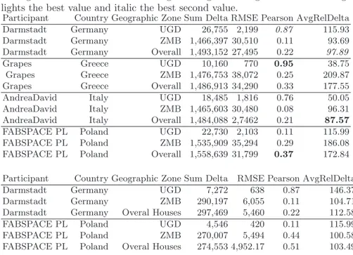
Table 1: Population estimation. UGD stands for Uganda while ZMB is for Zam-bia region. Overall is when considering both regions all together. Bold font high-lights the best value and italic the best second value.
Participant Country Geographic Zone Sum Delta RMSE Pearson AvgRelDelta Darmstadt Germany UGD 26,755 2,199 0.87 115.93 Darmstadt Germany ZMB 1,466,397 30,510 0.11 93.69 Darmstadt Germany Overall 1,493,152 27,495 0.22 97.89 Grapes Greece UGD 10,160 770 0.95 38.75 Grapes Greece ZMB 1,476,753 38,072 0.25 209.87 Grapes Greece Overall 1,486,913 34,290 0.33 177.55 AndreaDavid Italy UGD 18,485 1,816 0.76 50.05 AndreaDavid Italy ZMB 1,465,603 30,480 0.08 96.31 AndreaDavid Italy Overall 1,484,088 2,7462 0.21 87.57 FABSPACE PL Poland UGD 22,730 2,103 0.11 115.99 FABSPACE PL Poland ZMB 1,535,909 35,294 0.29 186.08 FABSPACE PL Poland Overall 1,558,639 31,799 0.37 172.84 Participant Country Geographic Zone Sum Delta RMSE Pearson AvgRelDelta Darmstadt Germany UGD 7,272 638 0.87 146.37 Darmstadt Germany ZMB 290,197 6,055 0.11 104.71 Darmstadt Germany Overal Houses 297,469 5,460 0.22 112.58 FABSPACE PL Poland UGD 4,546 420 0.11 115.99 FABSPACE PL Poland ZMB 270,007 5,494 0.44 100.58 FABSPACE PL Poland Overal Houses 274,553 4,952.17 0.51 103.49
Uganda. Again the best value was obtained by Greece (Pearson:0.95), the second best value was of the German team (Pearson:0.87).
Considering the AvgRelDelta we can say that in general the best population estimation approach is the one submitted by the Italian team (AvgRelDelta: 87.57).
4.2 Summary of participants’ approaches
The aim of this work was to estimate the population for selected areas in Uganda and Zambia with Sentinel-2 data.
The approaches used by the participants to tackle this challenge were diverse. In the case of Italy, the participants used an approach based on a convo-lutional neural network (CNN) that makes use of Sentinel 2 Imagery (bands 2,3,4,8) as well as LDS built up estimates provided by the Center for Interna-tional Earth Science Information Network (CIESIN). The LDS Built up esti-mates have a resolution of 30m and provide build up information as recent as 2014. The most recent estimates are based on Landsat 8.
In the case of Germany, the approach was based on diverse techniques of image classification. The participants used a subset of the bands provided by Sentinel 2 (bands 2,3,4 and 8) and also tested using only near infra-red band. The classification techniques used were supervised and unsupervised, using tools
as QGIS and Sentinel Tool Box (SNAP). As part of the approach, additional information from Sentinel 1 radar imagery was used.
In the case of Poland Railways approach to the number of buildings was done using radar images. The results obtained by estimating the number of buildings from radar imagery was more applicable. Optical data has been used to divide areas by type of building. The results obtained and their comparison to the number of buildings was very promising.
4.3 More evaluation
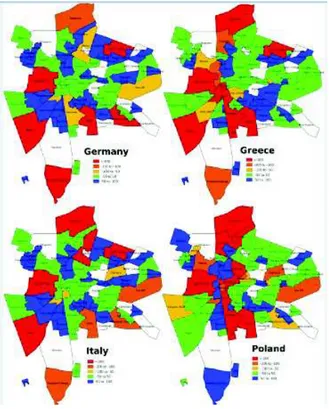
Fig. 1.Overview of the results submitted by the participating teams Team for the operational zones in Lusaka- Zambia.
Figure 1 depicts an overview of the results submitted by the participating teams. The maps depict the prediction errors divided by the ground truth pop-ulation for each operational zone. We divide the prediction errors in order to consider the great range of population counts among the operational zones. We used the relative delta as described in Section 3.2.
Operational zones in which the models have severely overestimated the pop-ulation (the models suggest more poppop-ulation that the real one) are depicted in red or orange. We consider severely overestimated results when the population estimation is more than 50% of the actual population. Areas in which the estima-tion is +/− 50% are depicted in green, while areas in which the models severely underestimated the population are depicted in blue. For this paper, a population estimation would be consider severely underestimated if it is less than 50% of the actual population.
We can see that there are areas overestimated by all the models: The In-dustrial area (West), Ngwerere (North) and Libala (South). In the case of the industrial areas, it seems that the proposed algorithms confused industrial build-ings for residential areas. In the case of Ngwere, and Libala, the residential areas have low density which was incorrectly evaluated by the algorithms.
On the other hand, we can see that there are other areas that have been underestimated by all the models: George, Lilanda, Desai, (at the West of the city), Chelston at the East, Chawama and Kuoboka at the South.
Most of the models underestimated the population in Makeni, except for the Polish team. This team also differentiated from the rest in an area comprised by Ngombe, Chamba Valley, Kamanga and Kaunda square (North East of the city), providing good estimates with the exception of Chudleigh, which was which was overestimated by all the teams, except for the Italian team.
In general, all the teams got their best results in an area near the center of the city, an area roughly defined by the Operational zones, Civic Centre, Rhodes Park, and in most cases Northmead (except for the Polish team who did not provide a good result for this zone).
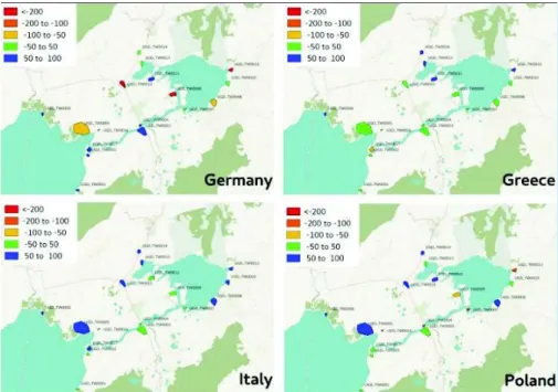
Figure 2 depicts the results of the participating teams for the operational zones in Uganda. As in the map depicting the operational zones located in Lusaka, the map depicts the zones with severe overestimation in red and or-ange (less than -50%), while it depicts the areas with severe underestimation in blue (more than 50%).
In the case of German team, they overestimated 5 of the 17 operational zones (depicted in orange and red) and underestimated 7 of the zones depicted in blue. The solution proposed by the Greek team has less overestimation, only one of the zones was overestimated. However, it severely underestimates 5 zones, while it has a good estimation for 11 zones. The submission of the Italian team, does not have any overestimation. However, it severely underestimates the population in 9 of the zones. The approach followed by the Polish team, produces mixed results. It severely underestimates the population in 5 zones while it underestimates it in 6.
5
Related work
Emerging technologies including mobile application, global positioning system and satellite images can create changes in development. Estimation of popula-tion using earth observapopula-tion and geospatial technologies can ease emergency
ser-Fig. 2.Overview of the results submitted by the participating teams, for the opera-tional zones in Uganda.
vices and humanitarian actions. For instance, providing emergency relief, tack-ling post-earthquake situation and tracking epidemic diseases like cholera needs up-to-date and geographically specific information. The accurate information a governmental organization and/or NGOs and/or other aided organization can have, the more they can save lives.
A couple of related works has been done to estimate population and make it atomize to avoid unnecessary expanses and time required in conventional cen-sus methods of estimating population. In their studies Florence A. Galeon [10] and Almeida et al. [1] underline the potentials of using high resolution Quick-bird images to estimate population in informal and semi-informal settlements in urban area. In another study, United Nations Statistics Division DESA [9] in-tegrated GPS, digital imagery and GIS technology to make the census mapping more accurate and efficient. Li and Weng [16] integrated Landsat ETM+ data with census data for estimation of population density of Indianapolis, Indiana USA. They incorporated spectral signatures, principle components, vegetation indices, fraction images, textures and temperature as predictive indicators to make a correlation analysis between remote sensing parameters and population. In the studies of Cheng et al. [5], Prosperie, [19] and Sutton [21] [22], the au-thors used “night satellite” imagery to estimate population according to the local densities of light sources. Dittakan et al. ’s studies [7] [8] used satellite images
from GeoEye 50m ground resolution data publicly available by Google Earth.In another studies Ilka et al. [20] used TM/Landsat5 and ETM+/Landsat7 data to estimate population of Belo Horizonte city in Brazil by generating statistical model.
There are also plenty of other studies that used high to moderate resolution satellite imagery to estimate population. There are relatively few studies on esti-mating population based on radar satellite data such as Henderson, F. and Xia, Z. elaborated radar applications in Urban Analysis, settlement detection and population estimation [11] [12], Balz, T. and Haala, N., interpreted high reso-lution SAR data using existing GIS data in urban areas to estimate population [3].
There are lots of other new satellites providing either commercial or free satellite images which can be also evaluated in the task of estimating the pop-ulation of an area. However, Sentinel-2 optical and Sentinel-1 radar satellites are free and moderately high resolution satellite imagery. In this ImageCLEF 2017 pilot task the prime objective was to precisely identify how powerful are Sentinel-2 imagery of 10m resolution.
6
Conclusion
This paper summarizes the pilot task introduced this year at image CLEF 2017 and that aims at estimating the population of a zone. Participants encountered various difficulties mainly linked to the nature of the images they had to use. The results that were obtained show that there is room for improvement using low resolution images for estimating the population in a zone although these images have the huge advantage of being free of use.
7
Acknowledgement
This project received funding from the European Unions Horizon 2020 Research
and Innovation programme under the Grant Agreement n693210. https://www.fabspace.eu/
References
1. C. M. Almeida, I. M. Souza, C. D. Alves, C. Pinho, M. N. Pereira, and R. Q. Feitosa. Multilevel object-oriented classification of quickbird images for urban population estimates. In Proceedings of the 15th annual ACM international sym-posium on Advances in geographic information systems, page 12. ACM, 2007. 2. H. Arenas, A. Baker, A. Bialczak, D. Bargiel, M. Becker, V. Gaildrat, F.
Car-bone, S. Heising, M. B. Islam, P. Lattes, C. Marantos, C. Menou, J. Mothe, A. Nzeh Ngong, I. S. Paraskevas, M. Penalver, P. Sciana, and D. Soudris. Fab-Spaces at Population Estimation (remote) Task ImageCLEF at the CLEF 2017 Labs. CLEF 2017 Labs Working Notes, 2017.
3. T. Balz and N. Haala. Interpretation of high resolution SAR data using existing GIS data in urban areas. Universit¨atsbibliothek der Universit¨at Stuttgart, 2005.
4. A. G. Barnston. Correspondence among the correlation, RMSE, and heidke forecast verification measures; refinement of the heidke score. Weather and Forecasting, 7(4):699–709, 1992.
5. K. Chen. An approach to linking remotely sensed data and areal census data. International Journal of Remote Sensing, 23(1):37–48, 2002.
6. F. Del Frate, J. Mothe, C. Barbier, M. Becker, R. Olszewski, and D. Soudris. Fab-Space 2.0: The Open-Innovation Network for Geodata-driven Innovation (regular paper). In International Geoscience and Remote Sensing Symposium (IGARSS), Fort Worth, Texas, USA, 23/07/2017-28/07/2017, juillet 2017.
7. K. Dittakan, F. Coenen, and R. Christley. Towards the collection of census data from satellite imagery using data mining: A study with respect to the ethiopian hinterland. In Research and Development in Intelligent Systems XXIX, pages 405– 418. Springer, 2012.
8. K. Dittakan, F. Coenen, R. Christley, and M. Wardeh. A comparative study of three image representations for population estimation mining using remote sensing imagery. In ADMA (1), pages 253–264, 2013.
9. U. N. S. Division. Integration of gps, digital imagery and gis with census mapping. ESA/STAT/AC.98/14, 2004.
10. F. Galeon. Estimation of population in informal settlement communities using high resolution satellite image. In XXI ISPRS Congress, Commission IV. Beijing, volume 37, pages 1377–1381, 2008.
11. F. Henderson and Z. Xia. Radar applications in urban analysis, settlement detec-tion and populadetec-tion estimadetec-tion. Manual of Remote Sensing, 2:759–761, 1998. 12. F. M. Henderson and Z.-G. Xia. SAR applications in human settlement detection,
population estimation and urban land use pattern analysis: a status report. IEEE transactions on geoscience and remote sensing, 35(1):79–85, 1997.
13. B. Ionescu, H. M¨uller, M. Villegas, H. Arenas, G. Boato, D.-T. Dang-Nguyen, Y. Dicente Cid, C. Eickhoff, A. Garcia Seco de Herrera, C. Gurrin, B. Islam, V. Kovalev, V. Liauchuk, J. Mothe, L. Piras, M. Riegler, and I. Schwall. Overview of ImageCLEF 2017: Information extraction from images. In CLEF 2017 Pro-ceedings, volume 10456 of Lecture Notes in Computer Science, Dublin, Ireland, September 11-14 2017. Springer.
14. M. B. Islam, M. Becker, D. Bargiel, K. R. Ahmed, P. Duzak, and N.-G. Emana. Sentinel-2 Satellite Imagery based Population Estimation Strategies at FabSpace 2.0 Lab Darmstadt. CLEF 2017 Labs Working Notes, 2017.
15. K. Koutsouri, I. Skepetari, K. Anastasakis, and S. Lappas. Population Estimation Using Satellite Imagery. CLEF 2017 Labs Working Notes, 2017.
16. G. Li and Q. Weng. Using landsat etm+ imagery to measure population density in indianapolis, indiana, usa. Photogrammetric Engineering & Remote Sensing, 71(8):947–958, 2005.
17. K. Pearson. Note on regression and inheritance in the case of two parents. Pro-ceedings of the Royal Society of London, 58:240–242, 1895.
18. A. Pomente and D. Aleandri. Convolutional Expectation Maximization for Popu-lation Estimation. CLEF 2017 Labs Working Notes, 2017.
19. L. Prosperie and R. Eyton. The relationship between brightness values from a nighttime satellite image and texas county population. Southwestern Geographer, 4:16–29, 2000.
20. I. A. Reis, V. L. Silva, and E. A. Reis. Adjusting population estimates using satellite imagery and regression models. Anais XV Simpsio Brasileiro de Sensoriamento Remoto, SBSR, pages 830–837, 2011.
21. P. Sutton. Modeling population density with night-time satellite imagery and GIS. Computers, Environment and Urban Systems, 21(3):227–244, 1997.
22. P. Sutton, D. Roberts, C. Elvidge, and K. Baugh. Census from heaven: An estimate of the global human population using night-time satellite imagery. International Journal of Remote Sensing, 22(16):3061–3076, 2001.