© Maha Abdelhalim, 2020
Estimating Flood Impact on Residential Values (Housing
Price), The Case of Laval (Canada), 1995-2007
Mémoire
Maha Abdelhalim
Maîtrise en aménagement du territoire et développement régional - avec
mémoire
Maître en aménagement du territoire et développement régional (M.ATDR)
ESTIMATING FLOOD IMPACT ON RESIDENTIAL
VALUES (HOUSING PRICE):
THE CASE OF LAVAL (CANADA): 1995-2007
Mémoire
Maha AbdelHalim
Sous la direction de :
Résumé
Cette thèse vise à améliorer notre compréhension du modèle hédonique et de son application sur les données des biens immobiliers afin d'étudier l'impact d'un événement / externalité / environnementale liée à la présence d'inondation sur la valeur des propriétés résidentielles. Étant donné que les données immobilières sont réparties dans l'espace et dans le temps, des "corrections" temporelles et spatiales sont nécessaires dans le processus de modélisation économétrique. La recherche prend appui sur l’équation de prix hédonique. L’analyse empirique recours également à l’estimateur de type différence de différences spatio-temporelles (STDID) afin d’étudier l’effet d’une inondation survenue en 1998 sur le prix des résidences dans la ville de Laval au Canada entre 1995-2007. Les résultats suggèrent que l’utilisation des informations sur les zones inondables dans le but d’évaluer l’impact des inondations sur les valeurs résidentielles n’est pas une approche nécessairement appropriée. Les conclusions suggèrent que la grande hétérogénéité des résultats notés dans la littérature n’est probablement pas étrangère à la façon de définir les résidences touchées par les inondations. Cela signifie que les recherches empiriques sur les effets des inondations sur la valeur immobilière mesurent en réalité la valeur liée à la perception du risque d'inondation et non l’effet réel de l'inondation. Les résultats suggèrent que les applications futures dans la littérature devront porter une attention particulière à la manière de définir les zones inondables et d’identifier les résidences réellement touchées.
Abstract
This thesis aims to improve our understanding of the hedonic pricing model and its application on real estate property data to investigate and estimate the impact of an environmental event/externality/disamenity of flood on residential property value. Since real estate data is spatially distributed over time, temporal and spatial ‘fixes’ are required in our econometric modelling. The paper builds on the classic hedonic pricing model. A spatiotemporal difference-in-differences (STDID) approach is adopted to investigate the effect of a flood event occurring in 1998 on housing price in Laval city in Canada between 1995-2007. Results suggest that relying on flood zones to investigate the effect of flood on housing price is not an accurate method. This conclusion suggests that most of the heterogeneity in the results found in the literature mainly comes from a bad identification of the houses really flooded. Thus, the usual empirical investigation of flood effects on real estate value measures the impact of flood risk (or risk perception) and not the real effect of flood. Implications of research for future work include the importance of use of a better delimitation of actual houses flooded for the empirical investigation of flood effect on housing price.
Table of Contents
Résumé ... iii
Abstract ... iv
Table of Contents ... v
List of Tables ... vii
List of Figures ... viii
Dedication ... ix Remerciements ... xi Foreword ... xii Introduction ... 1 Research Question ... 7 Assumption ... 7 Research Objectives ... 7 Challenges ... 8
Chapter 1 Literature Review ... 9
1.1 Literature on Flood Impact ... 9
Chapter 2 Analytical Approach & Methodology ... 21
2.1 History of Hedonics ... 21
2.2 Theoritical Foundations : The Hedonic Pricing Model (HPM)... 23
2.3 Disadvantages of the HPM ... 25
2.4 Research Methodology: Building on the Hedonic Price Function ... 26
2.4.1 The Standard Hedonic Price Function... 26
2.4.2 Estimating the Flood Effect ... 27
2.4.2.1 First : Creating the DID Estimator ... 28
2.4.2.2 Second : Creating the STDID ... 29
Chapter 3 Data and Case Study : The Flood Plains in Laval City ... 32
The Flood Plains in Laval City ... 32
Chapter 4 Results & Discussions ... 40
4.1 Research Results ... 40
4.2 Discussion ... 48
Research Originality ... 52
Research Limitations ... 53
Implications & Future Avenues of Research ... 53
List of Tables
Table 1.1 | Summary of Studies on the Influence of Flood on the Value of Real Estate ... 11
Table 2.1 | List of Variables Available in the Database. ... 34
Table 3.2 | Descriptive Statistics for Houses Inside and Outside the Flooding Zone (Large Zone) ... 39
Table 4.1 | Estimation Results with DID Specification Using OLS ... 42
List of Figures
Figure 0.1 |"Île-Mercier covered in floodwater in May 2017" (CBC News) ... 4
Figure 0.2 | “A submerged car in Sainte-Martha-sur-le-lac in 2019 (Montreal Gazette)... 5
Figure 0.3 | "Residents use boats to pick up possessions on a flooded street (Montreal Gazette) ... 6
Figure 2.1 | Haas (1922): Thesis Title Page and Forecasting Formula ... 22
Figure 3.1 | Spatial Distribution of the Transactions on the Laval City Map ... 33
Figure 3.2 | Flooded Streets (as in May 2017) (Laval.ca) ... 38
Dedication
To my father,
In loving memory…
To my husband, my kids and my mum,
A million years ago I read the eternal verses
of Robert Frost (1920)
named Mountain Interval,
Two roads diverged in a wood, and I—
I took the one less traveled by,
Remerciements
Firstly, I would like to thank my supervisor, Professor Jean Dubé, for his kind help and endless support. Mr. Dubé had the patience and kindness to introduce me to the difficult science of econometrics and to Stata. I am forever grateful.
Secondly, I would like to thank my colleague Diego Cardenas Morales for his kindness and continuous help. I would also like to thank Guy Morel, who had the kindness to help a total stranger, me, with all my Stata questions.
Finally, I would like to thank the Marine Environmental Observation, Prediction and Response Network (MEOPAR) for their financial support that made this research possible. This research is part of a research group (of which Prof. Dubé is member), titled, Comment passe-t-on à l'action avec les plans d'adaptation et de résilience? Projet de recherche en zone côtière et riveraine du Québec et de l'Ontario (2018-2021) and is funded by MEOPAR research grant.
Foreword
I begin with the words of Frederick V. Waugh, the father of the Hedonic pricing model, who spent a lifetime developing methods of economic research that he hoped would solve real life problems. Little did he know, that his research on vegetable price, will turn into the foundation of the most commonly used method in housing property valuation. Waugh, who was a founder of the econometric society, was quite concerned that econometrics was becoming too sophisticated to the extent that it became “irrelevant.
In his 1961 piece, The Place of Least Squares in Econometrics, he declared,
"I am not recommending 'empirical' work, which my dictionary defines as 'depending upon experience or observation alone, without due regard to science and theory.' Economic facts without theory are of little value. But neither is theoretical speculation without facts. What we need is more work that is truly econometric, i.e., that combines mathematics, economic theory, and statistical measurements to explain how the economy operates and to give the basis for usable economic predictions."
Abel (1988) describes this article saying that, “the point of his article is that a simple statistical technique is a perfectly valid one for forecasting. One does not necessarily need more elaborate models…This pioneering article has stood the test of time! “
So, I promise you, that we will try to capture the original spirit of econometrics, as envisioned by Waugh, and as a simple art of combining mathematics, statistical theory and economic theory to explain the economy, how it works and provide useful predictions for the service of everyday life and layman as well as municipal institution.
To embark on our journey into econometrics, in the simplified manner envisioned and championed by its founding father, we are going to use the simplest yet one among the most powerful of functions: The Hedonic Function.
The Famous HPM
Through a long history that is almost a century old, the classic hedonic pricing model or (HPM) has evolved to become the method of preference for estimating the contribution of urban externalities to price of a real estate property. Mills (2000) states that the use of
hedonics was dragged to be applied to housing research in the early seventies (though it was applied earlier to other research areas, like vegetables and cars).
But what is hedonic to begin with? The term ‘Hedonic’ is derived from Hēdonē, which is Greek (Wikipedia) and is the root of the English hedonism that “is the search for pleasure.”(Stanford.edu) In an economic sense, hedonic “means of or related to utility.”
Hedonic prices are the implicit prices of characteristics/attributes of differentiated goods that compose the bundle of a complex good. They are derived by observing the joint variation of the good/product price and the bundles of a good’s characteristics. (Zhao, 2008).
The idea is quite simple. A good explanation is provided by Malpezzi et al. (1980) who compared housing to a grocery bundle in the sense that some of grocery bundles are quite bigger than the others and surely contains different items. If we reflect this view on housing, a house is a grocery bundle composed of bedroom items, bathrooms and amenities of all sorts. Each house has its particular and distinctive bundle that sets it apart from the other houses, but unlike groceries, we cannot observe or evaluate the price of those individual features/characteristics/attributes directly(Sirmans et al., 2005), e.g. the price/value of an atrium relative to an overall value of a house. Hedonic modeling is useful since it helps price these attributes by conducting a “multiple regression analysis on a pooled sample of many dwellings.” As stated earlier, the genius of the hedonic pricing models is that through it, we can measure the effect of these otherwise unmeasurable attributes on the overall price/transaction. The model returns the coefficients (that are generated by a conduction of a regression analysis), which represent the mean marginal implicit price for each attribute (Monson, 2009).
Using this simplified model, we can calculate/estimate “what proportion of a home’s price is accounted for by structural characteristics and characteristics of the site and neighborhood.” As such, using the hedonic function we can provide “monetary measures of the value of school quality, the cost of air pollution” (Arnott and McMillen, 2006) and in our case the effect of flood.
Hedonic pricing models are very common and are used extensively in environmental evaluation to value/estimate local amenities and is especially used to estimate the pollution damage (see Bayer et al., 2009, OECD, 2013). The hedonic pricing model is largely used to evaluate the price of goods for which there exists no explicit market. We use it here in this thesis for the environmental evaluation of flood effect on housing price (as an externality).
I remember when I first had to write about an alleged hedonic pricing model, which sounded very terrifying and very Greek, I hid in office, enrolling on econometric courses on Coursera, studying endlessly day and night. I am not here by coincidence. But why didn’t I hear about hedonics before? Unfortunately, despite its importance, urban economics is not celebrated well enough in urban planning circles. Darmanie (2019) writes a commentary named Urban planning, please meet urban economics, in which he condemns the fact that system of urban planning “seemingly operates in isolation from economic realities.” He quotes Alain Bertaud, “we are facing a strangely paradoxical situation in the way cities are managed: the professionals in charge of modifying market outcomes through regulations (planners) know very little about markets, and the professionals who understand markets (urban economists) are seldom involved in the design of regulations aimed at restraining these markets.” I think that urban economics should be more accentuated in a planner’s education. Economics is key to all planning decisions.
At the beginning of my econometric path, I read a paper by Devaux et al. (2017) (to which I was introduced by my supervisor Professor Dubé and of which he is a co-author of the paper submitted) which was on the anticipation and post-construction impact of a metro extension on residential values: The case of Laval (Canada): 1995-2013. In this paper a spatial difference-in-difference (SDID), based on RS-repeat sales approach (which has HPM at its foundation), was used to isolate the effect of proximity to a new infrastructure (metro) on residential property value. Something certainly clicked inside that brain of mine. This was not just mathematics nor statistics, it was more. It was econometrics. I was charmed by the simplicity of hedonics: a house is a bundle of nonmarket attributes, plus a beta or minus a theta, I get it. Genius. Next, I came across a pivotal text by Jean Dubé and Diègo Legros, Spatial Econometrics Using Microdata. It was logic and to the point. Gradually, I felt myself shift from a qualitative to a quantitative mindset academically. Now Cerdà and Haussmann bore me.
Through the use of a hedonic function method that describes a hedonic model we can quantify qualitative or non-market attributes or characteristics of a certain product or good, that is in the case of this research, a real estate property or a housing good. This quantification of the qualitative, acts as a necessary hinge/bridge/link that ends in a triumph of sound policy and decision-making on the territory. Hedonics allow the planner to estimate, these otherwise inestimable, urban externalities that include pollution, distance to public
transport or being in a flood zone (as is the case in this research). As such, hedonics acts as the lost hinge between the facets of the very complicated tale of planning.
The article presented in this thesis is titled, Flood Impact on Residential Values (Housing
Price): The Case of Laval (Canada), 1995-2007. In this paper Hedonic pricing model was
used as a foundation for a differences (DID) and a spatial difference-in-differences (SDID) estimators to estimate the effect of an environmental disamenity/externality which is the effect of a flood event that occurred in Laval City in 1998. The paper was submitted on the 2nd of December to the Journal of Environmental Economics
and Management (JEEM). I am the first author of the paper and I co-author with my supervisor, Prof. Jean Dubé (Université Laval) and Prof. Nicolas Devaux (UQÁR). Under the supervision of my supervisor Prof. Dubé, I was involved in the empirical statistical analysis involving the use of the ArcMap and Stata software as well as conducting the literature review as well as participating in writing the research paper.
Now, it is time to introduce the research that will then be followed by an explanation of the theoretical and historical foundations of the hedonics that I present in the next chapter. I hope the reader finds in hedonics the same compelling power that has been inspiring econometric research for decades.
I
ntroduction
City life involves a complex array of attractive/positive and unattractive/negative features, which are called urban externalities and that are described as being unpriced nonmarket effects. Examples of urban externalities include, noise, traffic congestion, pollution, crime, but also natural disasters such as floods, fire, earthquakes and erosion. (Dubé et al., 2020). Yet, measuring urban externalities remains quite the challenge (Verhoef and Nijkamp, 2003).
This thesis aims to measure the implicit value of a 1998 flood event as an urban externality through real estate market data of Laval city in the province of Québec in Canada. Observations that include property transactions and information are used to estimate (not calculate) the nonmarket value of environmental disamenities of flood events as urban externalities. In the case of this thesis we are using single-family houses in Laval to investigate the effect of a 1998 flood event on housing price.
This topic (i.e. measuring flood as an urban externality) has come to prominence since floods have been generally quite the hot topic lately. Climate change, the environmental crisis of our modern times, has increased the occurrence of flood events and aggravated such a problem (Békés et al., 2016; Bélanger et al., 2018). A warmer atmosphere has a greater capacity to hold water, which increases the chance of the occurrence of floods. As a result, flood events are expected to occur more frequently in the future (IPCC, 2007; Daniel et al., 2009) and floods remain one of the most recurrent natural disasters world-wide. Canada is no exception.
The Canadian territory has been hit by multiple floods lately. The recurrence of severe episodes of weather (which are of normal occurrence in Canada) could lead to the worsening of the situation even further (Bélanger et al., 2018). Thus, it is not surprising to know that floods are the natural disasters that cost the most in Canada (Sandink et al., 2010). There is an average loss of 1-2 billion Canadian dollars each year (Jakob and Church, 2011). Since floods cause such losses, it is essential to identify the areas that are exposed to flood events, to assess/consider the potential losses and to respond to risks. To achieve this aim, government agencies, insurance companies and emergency managers (on the local level) need tools to estimate the expected losses to the building stock as well as the infrastructure in floodplains. Oubennaceur et al. (2018) and Beltrán et al. (2019) support this view and
insist that the increase in number of flood events as a result of climate change and the continuous planning in floodplains, means that we need to understand the effect of flood on households. This is even more important according to the fact that the literature on this topic is far from being convincing regarding the large span of estimated effect (between 61.0% to a -75.5% price premium).
This vast heterogeneity of results suggests a relationship between floods and housing that has its own specificity and is quite indicative of the state of uncertainty in the literature on the effect of floods on housing price. Bélanger et al. (2018) state that literature shows “a large amount of disagreement about the level of flood risk” with a vast contrast of results. The authors also state that the contradictory results in the literature can be rationalized by the fact that a flood is a heterogeneous and “local “event that has consequences that vary with many factors that include geographical and hydrological considerations, the water resistance of the flooded property as well as the availability of an overland flood insurance. As such the results of a flood event is localized and ‘specific’ to this localization (i.e. not yielding to generalization).
Yet there is another plausible explanation, which is that the results are often tied to the choice of floodplains, which can be misleading. Aliyu et al. (2016) highlight the contradictory results of the global inquiry on the impact of flood disclosure on the value of property and that this contradiction is often acknowledged in the literature. They state that there is one finding that is agreed upon, which is that the event of flood itself rather than being inside a floodplain is probable to have a bigger impact on the value of property. Beltrán et al. (2017) also describe an inconsistency of results of previous studies stating that numerous studies have analyzed the location effect of being in a 500 or 100-year floodplain but say that results are inconsistent, and they point to a presence of a price premium more “than the expected discount.” Flood events rather than floodplains are most probably more influential on property value.
But what are floods really all about? In the mentality of the public, a flood event is an overflow of rain or a river. To be more precise, in scientific terms, floods are phenomena of nature that happen when lakes, streams and rivers overflow their natural banks. As natural disasters, a flood is defined by the damage it causes to people or property (West, 2010). The definition of a flood as a natural disaster is related to the fact that people inhabit flood prone areas. A flood event in itself as a natural phenomenon (as represented by a waterbody exceeding its natural banks) is not to be labeled as a natural disaster. But it is the presence
of people and property in those flooded areas that transform it to a natural disaster (Montz, 1992b). Yet, flood areas are considered attractive and a pulling force for human settlement because of human convenience for a plenty of various reasons that include the attractive view, transportation, water supply and the rich agricultural soil (Eleuterio, 2012).
Since floods are natural disasters that have significant consequences (Békés et al., 2016), flood risk is an important land use policy issue. (Beltrán et al., 2019). Public policy is now turning towards intervention since flood events involve considerable costs, including a reduction of housing price (Békés et al., 2016). Moreover, the effect of flood on housing price is used as justification for municipal spending and has serious implications on public spending on flood mitigation measures and on urban design.
The recent flood events of 2017 and 2019 occurring across the province of Québec have raised the attention to study not only the economic but also the psychological and sociological impact of flood on local population. Those major events happen only a few years after that the Richelieu River floods that happened in 2011 and which was a result of a consecutive series of water level increase. These events began at the end of April of 2011. They caused an overflow of the Richelieu River in Quebec and Lake Champlain in the US. The water level increases were a result of a record snowfall that was followed by a snowmelt simultaneously occurring with intense spring rain (Castle, 2013).
In 2017, the city of Laval was hit by a flood event that was described as the worst in 100 years. The rising rivers flooded houses in both Montreal and Laval (The Suburban). The overflowing flood of the river wrecked a bridge in Île Verte. The Rivière des Mille Îles, the Rivière des Prairies and the Lake of Two Mountains are all connected to the Ottawa River. When the Ottawa River floods, like it did in 2017, all the linked water bodies suffered high-water levels.
In spring of 2017, hundreds of houses in the West Island of Montreal were flooded and damaged by the high waters. Figure (0.1) shows the Île Mercier that was submerged.
Fig (0.1): “Île-Mercier was covered in floodwater in May 2017 “(CBC News).
Situations like this may become more frequent with climate change, experts warn, and it’s time to plan for flooding (Paul Chiasson/Canadian Press)” (CBC News).
In 2019, there were recurrent waves of flood in Laval. More than 10,000 Quebecers left their homes as a result of the spring floods that happened in April. Across Quebec, 10,149 left their homes: 6,681 homes were flooded while 3,458 houses were cut off their communities (Montreal Gazette).
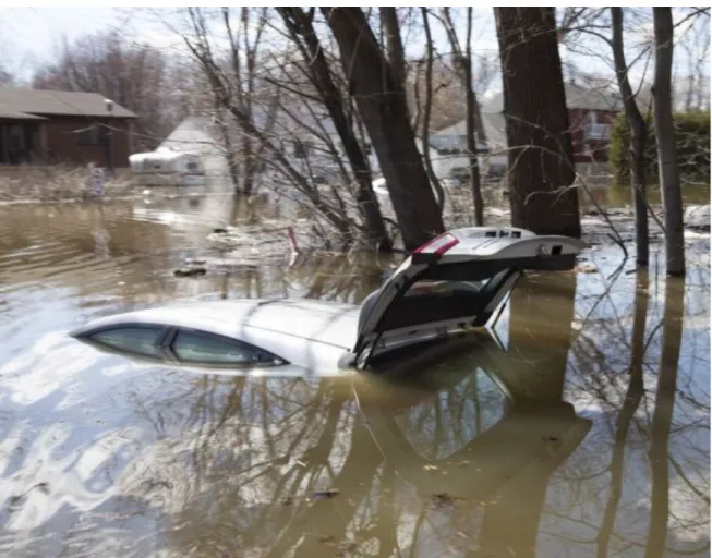
The impact was particularly strong in Sainte -Marthe-sur-le-Lac. In April 2019, thousands of residents were forced from their homes when a dike ruptured in Sainte -Marthe-sur-le-Lac (which is a community 40 km northwest Montreal). The dike burst, as a result of spring flooding, forcing an evacuation of thousands of inhabitants. Firemen helped the evacuation. The Red Cross came to the rescue. Francois Legault, Quebec prime minister, pledged $1 million from Quebec province to the Red Cross to help the relief efforts. Water rose very quickly to the extent that parked cars were totally submerged. In Sainte -Marthe-sur-le-Lac, more than 5,000 residents were evacuated from their houses using an amphibious vehicle that is owned by the SQ (Sûreté du Québec) police service (CTV News). Many say that they lost everything in mere minutes (Global News). 27 houses were flooded, and 50 streets were
covered by 1-2 meters of water. At the time, Quebec officials stated that 5,584 homes were flooded and 3,188 were actually surrounded by water. As a result, 7,683 people were forced out of their houses and 50 landslides were reported (CTV News).
Figure (0.2): “A submerged car is seen in Sainte-Marthe-sur-le-Lac. Quebec April 30,
Figure (0.3): “Residents use boats to pick up possessions on a flooded street in
Sainte-Marthe-sur-le-Lac. Quebec April 30, 2019” (Montreal Gazette).
To sum up, the flood events of 2017 and especially the more recent one in 2019, occurring in different parts of Quebec, have made news as well as earlier flood events along the Richelieu River in 2011. Such a recurrence of flood events has meant that it is important to study the effect of flood on housing price. This is because such recurrence, which made the headlines, confirms that the perception of risk is quite elevated. Yet, there are contrary claims that about half of flood zone residents in Quebec aren’t aware that they live in flood zones “or they brush away the risk,” and that municipalities “are not even planning for the changes that are happening with climate change” (King, 2019 in CBC News). In addition, current flood mapping is incomplete, which complicates results of research and aggravates the problem. Olivier (2019) cites Professor Pascale Biron, who is an expert in river dynamics at Concordia University and who calls for a “more holistic approach to watersheds,” arguing that provincial government is responsible for the current crisis because it allowed the control
of flood maps to be in the hand of municipalities (which happened in the early 2000). Professor Biron states that the municipalities are “not necessarily the best entity to manage this…[since]…they have sort of a conflict of interest with property taxes and development in potentially risky zones.” Biron states that “improvements are needed in how mapping is tackled” and that the solution to floods “comes down to how we map flood risks” (Global News).
Literature indicates that the effect of flood is not to be automatically assumed as negative (since the effect of flood on housing price ranges from positive to negative across different geographical areas). As such, all the aforementioned contradictions give rise to the research question, assumptions, objectives and challenge.
R
esearch
Q
uestion
Specifically, the research will concentrate on the case of the city of Laval (because we have the data to deal with this issue). The investigation is among the first to be done in Québec. It is a good starting point to investigate the possible economic outcome for households, but also for municipality since fiscal revenues is directly related to house values. Finally, since the literature presents a wide range of results both negative to positive effect, then it is important to study the exact effect of flood on housing price in Laval. As such the research question is: What was the impact of the Flood event that occurred in the city of Laval in 1998 on housing (single-family) price?
A
ssumption
Economic theory suggests that externalities are internalized into real estate prices. As such, the presence of flood, as a negative externality, should be incorporated in single-family housing price and the ones that are more likely to face flood should be sold with a negative premium in response to flood. And since the effect of flood is quite localized and not yielding to generalizations then it is quite logical that we study the flood effect on housing price. Thus, the study aims at testing the following assumption: there exists a negative price premium related to being inside a flooding zone.
R
esearch
O
bjectives
This research aims to estimate the impact of the flood risk on housing values for houses located close to the St-Lawrence river within the island of Laval using 6,646 transactions of
single-family houses that are collected between 1995 and 2007. To do so, the research aims to decompose the risk perception as internalized by the housing market of being inside versus outside the flood zones (versus being in flooded streets) controlling for proximity to water to show the effect of the flood event in its mean and temporal effect as well as correcting for spatial autocorrelation.
C
hallenge
The challenge in this research is to find a method that accurately measures the effect of floods on housing price. In the literature, there is no common consensus on the magnitude of the flood impact on housing price. As stated earlier, floods are the natural disasters that cost the most in Canada (Sandink et al., 2010). Floods cost on average 1-2 billion Canadian dollars per year (Jakob and Church, 2011). Thus, they are an important land use policy issue (Beltrán et al., 2019). About 80% of municipalities in Quebec have to deal with floods. (King, 2019 in CBC News). However, the literature is also imprecise on the impact of flood on real estate prices, with a range of estimation that vary between a 61.0% to a -75.5% price premium. Thus, it is important to investigate (estimate) their exact impact on housing price.
C
hapter 1:
L
iterature
R
eview
The hedonic pricing model (HPM), as characterized by Rosen (1974), has a long history of trying to isolate the (marginal) contributions of amenities, both intrinsic and extrinsic, on house prices. Many characteristics are related to the house price determination process. Flood is considered as part of extrinsic amenities. On the one hand, proximity to water is a positive amenity since it is associated with a calm, nice view and life style. On the other hand, living close to water has also some drawbacks, such as the possibility of facing flood and natural disasters. Thus, the equilibrium between those two opposite effects depends on how the market perceives this arbitrage. It is also certain that the perception is highly related to personal experience, such as living or remembering flood events, but also to the relative risk of experiencing such a disaster.
1.1
L
iterature on
F
lood
I
mpact
Beltrán et al. (2019) classify the literature on the empirical investigation of the impact of flood into four main groups. The first group uses standard HPM to compare the property price inside versus outside a floodplain. The price differential is assumed as the flood risk implicit price in a housing market (MacDonald et al., 1987; Donnelly, 1989; Speyrer and Ragas, 1991; Bin, 2004; Bin and Kruse, 2006; Rambaldi et al., 2012; Meldrum, 2015). The second group studies the effect of flood on property price that is located inside a floodplain using difference-in differences (DID) estimators to analyse a price differential in the case of being in a floodplain location and before and after a flood event for those that have been flooded (Bin and Polasky, 2004; Hakkstrom and Smith, 2005; Kousky, 2010; Atreya et al., 2013). A third group of studies analyzes the impact of flood on property prices in inundated areas. Information on such areas is used to analyse the price impact of flood damage on affected properties (Daniel et al., 2009; Atreya and Ferreira, 2015). Finally, the fourth group of studies focuses on the effect of construction of flood defence and beach nourishment on property prices (Beltrán et al., 2018a; 2018b; Dundas, 2017; McNamara et al., 2015; Qiu and Gopalakrishnan, 2018).
Intuitively, having recently faced floods is expected to have a negative effect on the value of affected property. Also measures taken as a means to protect flood prone areas are expected to have a positive effect on the value of property (Montz, 1992). In the most basic
of terms, economic theory proposes that, other things being equal, the property price would suffer a discount as a result of being located in a floodplain, since this natural disaster engenders economic costs. Yet, surveying existing evidence reveals that such a price discount lies between a 61.0% to a -75.5% price premium (as is shown in Table 1.1). This range is quite indicative of the state of uncertainty on the effect of floods on housing price. In the case of a housing market that is efficient, property located in a floodplain should have a lower price than that of an equivalent property that is outside the floodplain. However, the market has a (limited) memory that is not necessarily persistent over many years (Atreya et al., 2013; Bin and Landry, 2013), and such a negative impact can well be put aside with time.
Bélanger et al. (2018) report that existing literature shows “a large amount of disagreement about the level of the flood risk” with a vast contrast of results. While there are papers that show no price discount at all as a result of flood risk (Bialaszewski and Newsome, 1990), others report more than 10 % discount (Donnelly, 1989; MacDonald et al., 1990). Such diverging results can be partially rationalized by a number of factors that include the fact that a flood is a heterogeneous local event that has consequences varying with geographical as well as hydrological considerations, the properties’ water resistance and the availability of an overland flood insurance (Bélanger et al., 2019).
Aliyu et al. (2016) also highlight the contradictory results of the global inquiry on the impact of flood disclosure on the value of property and that it is often acknowledged in the literature. He states that there is one finding that is agreed upon and that is that the event of flood itself rather than being inside a floodplain is probably to have a bigger impact on the value of property. Beltrán et al. (2017) also describe an inconsistency of results of previous studies stating that numerous studies analyzed the location effect of being in a 500 or 100-year floodplain but say that results are inconsistent and that they point to a presence of a price premium more “than the expected discount.”
11
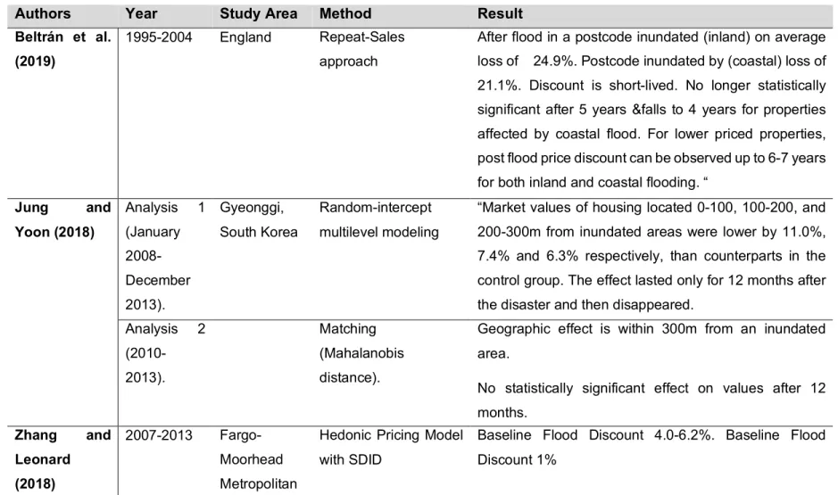
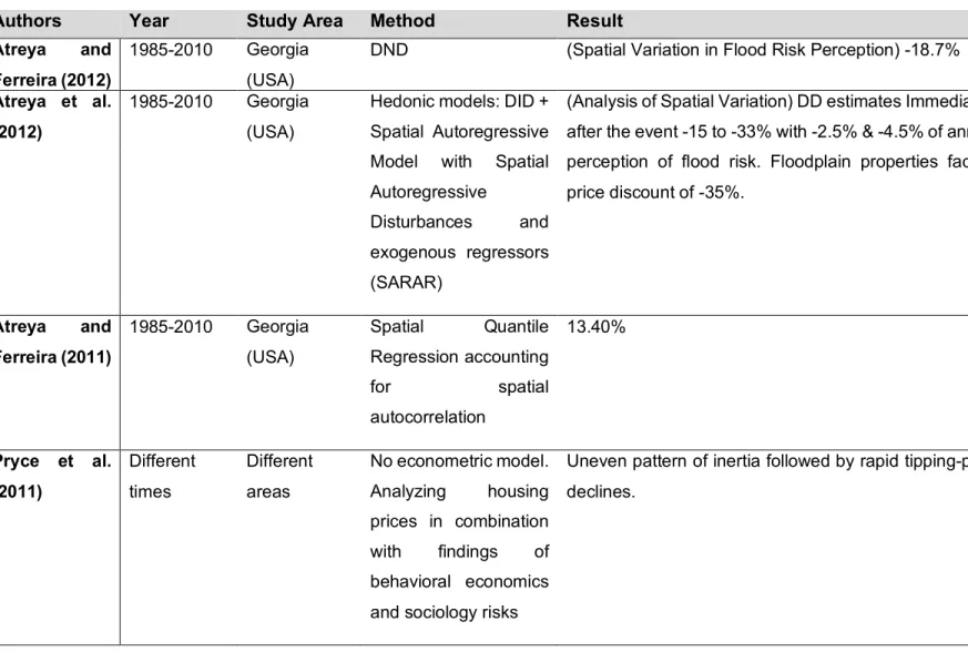
Table 1.1 | Summary of Studies on the Influence of Flood on the Value of Real Estate
(Adapted after Zhang and Leonard, 2018, Beltrán et.al, 2017; Aliyu et. al, 2016 and Kropp (2012)Authors Year Study Area Method Result
Beltrán et al. (2019)
1995-2004 England Repeat-Sales approach
After flood in a postcode inundated (inland) on average loss of 24.9%. Postcode inundated by (coastal) loss of 21.1%. Discount is short-lived. No longer statistically significant after 5 years &falls to 4 years for properties affected by coastal flood. For lower priced properties, post flood price discount can be observed up to 6-7 years for both inland and coastal flooding. “
Jung and Yoon (2018) Analysis 1 (January 2008- December 2013). Gyeonggi, South Korea Random-intercept multilevel modeling
“Market values of housing located 0-100, 100-200, and 200-300m from inundated areas were lower by 11.0%, 7.4% and 6.3% respectively, than counterparts in the control group. The effect lasted only for 12 months after the disaster and then disappeared.
Analysis 2 (2010-2013). Matching (Mahalanobis distance).
Geographic effect is within 300m from an inundated area.
No statistically significant effect on values after 12 months. Zhang and Leonard (2018) 2007-2013 Fargo-Moorhead Metropolitan
Hedonic Pricing Model with SDID
Baseline Flood Discount 4.0-6.2%. Baseline Flood Discount 1%
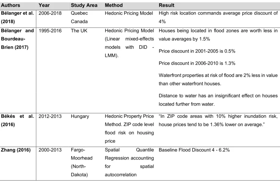
Table 1.1 | Summary of Studies on the Influence of Flood on the Value of Real Estate
(Adapted after Zhang and Leonard, 2018, Beltrán et.al, 2017; Aliyu et. al, 2016 and Kropp (2012)Authors Year Study Area Method Result
Bélanger et al. (2018)
2006-2018 Quebec Canada
Hedonic Pricing Model High risk location commands average price discount of 4%
Bélanger and Bourdeau-Brien (2017)
1995-2016 The UK Hedonic Pricing Model (Linear mixed-effects models with DID - LMM).
Houses being located in flood zones are worth less in value averages by 1.5%
Price discount in 2001-2005 is 0.5% Price discount in 2006-2010 is 1.3%
Waterfront properties at risk of flood are 2% less in value than other waterfront houses.
Distance to water has an insignificant effect on houses located further from water.
Békés et al. (2016)
2012-2013 Hungary Hedonic Property Price Method. ZIP code level flood risk on housing price
“In ZIP code areas with 10% higher inundation risk, house prices tend to be 1.36% lower on average.”
Zhang (2016) 2000-2013 Fargo-Moorhead (North-Dakota) Spatial Quantile Regression accounting for spatial autocorrelation
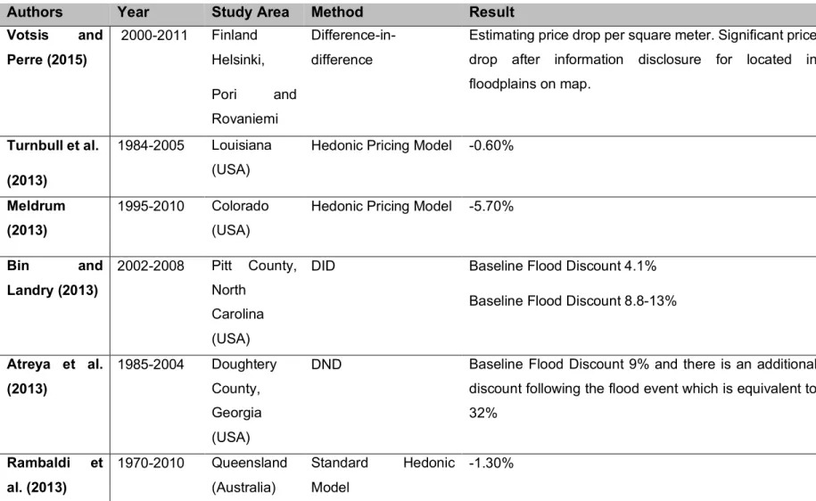
Table 1.1 | Summary of Studies on the Influence of Flood on the Value of Real Estate
(Adapted after Zhang and Leonard, 2018, Beltrán et.al, 2017; Aliyu et. al, 2016 and Kropp (2012)Authors Year Study Area Method Result
Votsis and Perre (2015) 2000-2011 Finland Helsinki, Pori and Rovaniemi Difference-in-difference
Estimating price drop per square meter. Significant price drop after information disclosure for located in floodplains on map.
Turnbull et al. (2013)
1984-2005 Louisiana (USA)
Hedonic Pricing Model -0.60%
Meldrum (2013)
1995-2010 Colorado (USA)
Hedonic Pricing Model -5.70%
Bin and Landry (2013) 2002-2008 Pitt County, North Carolina (USA)
DID Baseline Flood Discount 4.1% Baseline Flood Discount 8.8-13%
Atreya et al. (2013) 1985-2004 Doughtery County, Georgia (USA)
DND Baseline Flood Discount 9% and there is an additional discount following the flood event which is equivalent to 32% Rambaldi et al. (2013) 1970-2010 Queensland (Australia) Standard Hedonic Model -1.30%
Table 1.1 | Summary of Studies on the Influence of Flood on the Value of Real Estate
(Adapted after Zhang and Leonard, 2018, Beltrán et.al, 2017; Aliyu et. al, 2016 and Kropp (2012)Authors Year Study Area Method Result
Atreya and Ferreira (2012)
1985-2010 Georgia (USA)
DND (Spatial Variation in Flood Risk Perception) -18.7%
Atreya et al. (2012)
1985-2010 Georgia (USA)
Hedonic models: DID + Spatial Autoregressive Model with Spatial Autoregressive
Disturbances and exogenous regressors (SARAR)
(Analysis of Spatial Variation) DD estimates Immediately after the event -15 to -33% with -2.5% & -4.5% of annual perception of flood risk. Floodplain properties face a price discount of -35%. Atreya and Ferreira (2011) 1985-2010 Georgia (USA) Spatial Quantile Regression accounting for spatial autocorrelation 13.40% Pryce et al. (2011) Different times Different areas No econometric model. Analyzing housing prices in combination with findings of behavioral economics and sociology risks
Uneven pattern of inertia followed by rapid tipping-point declines.
Table 1.1 | Summary of Studies on the Influence of Flood on the Value of Real Estate
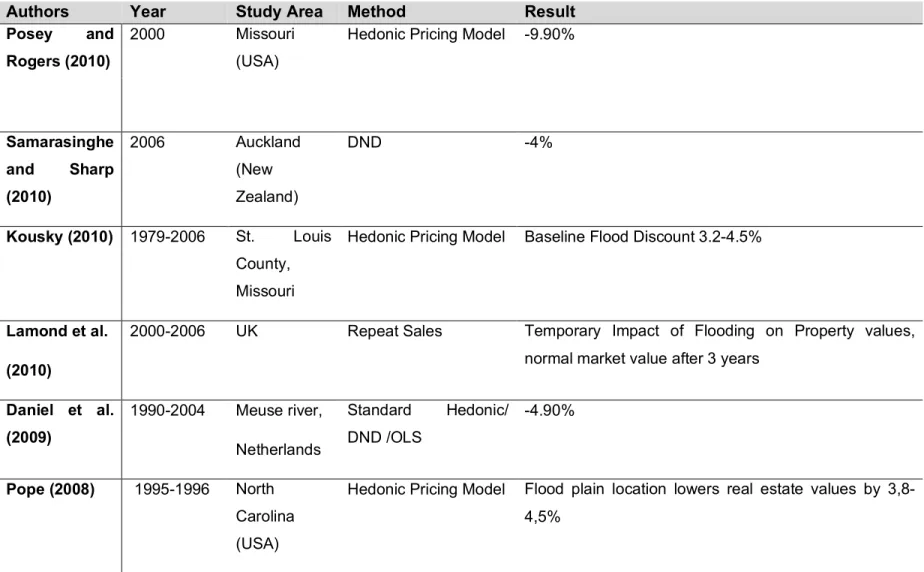
(Adapted after Zhang and Leonard, 2018, Beltrán et.al, 2017; Aliyu et. al, 2016 and Kropp (2012)Authors Year Study Area Method Result
Posey and Rogers (2010)
2000 Missouri (USA)
Hedonic Pricing Model -9.90%
Samarasinghe and Sharp (2010) 2006 Auckland (New Zealand) DND -4% Kousky (2010) 1979-2006 St. Louis County, Missouri
Hedonic Pricing Model Baseline Flood Discount 3.2-4.5%
Lamond et al. (2010)
2000-2006 UK Repeat Sales Temporary Impact of Flooding on Property values, normal market value after 3 years
Daniel et al. (2009) 1990-2004 Meuse river, Netherlands Standard Hedonic/ DND /OLS -4.90% Pope (2008) 1995-1996 North Carolina (USA)
Hedonic Pricing Model Flood plain location lowers real estate values by 3,8-4,5%
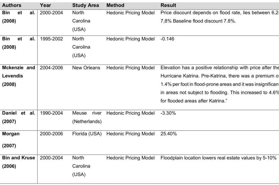
Table 1.1 | Summary of Studies on the Influence of Flood on the Value of Real Estate
(Adapted after Zhang and Leonard, 2018, Beltrán et.al, 2017; Aliyu et. al, 2016 and Kropp (2012)Authors Year Study Area Method Result
Bin et al. (2008)
2000-2004 North Carolina (USA)
Hedonic Pricing Model Price discount depends on flood rate, lies between 6,2-7,8% Baseline flood discount 7.8%.
Bin et al. (2008)
1995-2002 North Carolina (USA)
Hedonic Pricing Model -0.146
Mckenzie and Levendis (2008)
2004-2006 New Orleans Hedonic Pricing Model Elevation has a positive relationship with price after the Hurricane Katrina. Pre-Katrina, there was a premium of 1.4% per foot in flood-prone areas and it was insignificant in areas not subject to flooding. This increased to 4.6% for flooded areas after Katrina.”
Daniel et al. (2007)
1990-2004 Meuse river (Netherlands)
Hedonic Pricing Model -3.30%
Morgan (2007)
2000-2006 Florida (USA) Hedonic Pricing Model 25.40%
Bin and Kruse (2006)
2000-2004 North Carolina (USA)
17
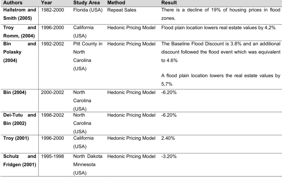
Table 1.1 | Summary of Studies on the Influence of Flood on the Value of Real Estate
(Adapted after Zhang and Leonard, 2018, Beltrán et.al, 2017; Aliyu et. al, 2016 and Kropp (2012)Authors Year Study Area Method Result
Hallstrom and Smith (2005)
1982-2000 Florida (USA) Repeat Sales There is a decline of 19% of housing prices in flood zones.
Troy and Romm, (2004)
1996-2000 California (USA)
Hedonic Pricing Model Flood plain location lowers real estate values by 4,2%
Bin and Polasky (2004) 1992-2002 Pitt County in North Carolina (USA)
Hedonic Pricing Model The Baseline Flood Discount is 3.8% and an additional discount followed the flood event which was equivalent to 4.6%
A flood plain location lowers the real estate values by 5,7%
Bin (2004) 2000-2002 North Carolina (USA)
Hedonic Pricing Model -6.20%
Dei-Tutu and Bin (2002)
1998-2002 North Carolina (USA)
Hedonic Pricing Model -6.20%
Troy (2001) 1996-2000 California (USA)
Hedonic Pricing Model 2.40%
Schulz and Fridgen (2001) 1995-1998 North Dakota Minnesota (USA)
Table 1.1 | Summary of Studies on the Influence of Flood on the Value of Real Estate
(Adapted after Zhang and Leonard, 2018, Beltrán et.al, 2017; Aliyu et. al, 2016 and Kropp (2012)Authors Year Study Area Method Result
Harrison et. al. (2001)
1980-1997 Florida (USA) Hedonic Pricing Model Flood plain location: discount bet. $985 to $2,100
Bartosova et al. (1999)
1995-1998 Wisconsin (USA)
Hedonic Pricing Model -1.60%
US Army Corps of Engineers (1998)
1988-1993 Texas (USA) Hedonic Pricing Model -2.90%
Speyrer and Ragas (1991)
1971-1986 Louisiana (USA)
Hedonic Pricing Model -9.80%
MacDonald et al. (1990)
1988 Monroe. Louisiana
Hedonic Pricing Model Baseline Flood Discount 7%
Bialszewski and Newsome (1990)
1987-1989 Alabama (USA)
Hedonic Pricing Model 0%
Shilling et al. (1989)
1982-1984 Louisiana (USA)
Hedonic Pricing Model -7.60%
Donnelly (1989)
1984-1985 Wisconsin (USA)
Table 1.1 | Summary of Studies on the Influence of Flood on the Value of Real Estate
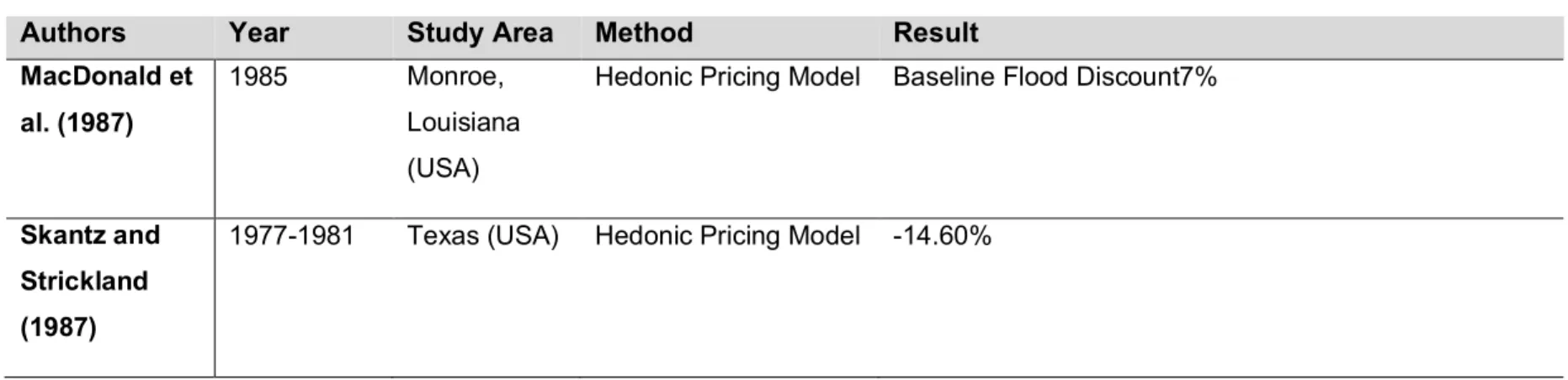
(Adapted after Zhang and Leonard, 2018, Beltrán et.al, 2017; Aliyu et. al, 2016 and Kropp (2012)Authors Year Study Area Method Result
MacDonald et al. (1987)
1985 Monroe,
Louisiana (USA)
Hedonic Pricing Model Baseline Flood Discount7%
Skantz and Strickland (1987)
Atreya et al. (2013) and Bin and Landry (2013) claim that the property price discount in response to a flood event “fades away between four to nine years after the flood.“ Aliyu et al. (2016) state that the empirical findings derived from their extensive review of literature revealed that the concerns of the owners of residential property at risk of being flooded regarding the long-term loss of value of their property, are mostly unfounded. Discounts in price are observed in areas that are recently flooded but they remain temporary. Montz (1992) state that his research results show that flood devalues property on the short-term. Yet, as the time from the flood event increases, the effect of the flood diminishes till it becomes insignificant and eventually there might be no observable effect at all.
C
hapter 2:
A
nalytical
A
pproach & Methodology
In this chapter the researcher introduces the research methodology, beginning with the theoretical foundations on which the analytical approach is built its disadvantages and its origins. This is followed by a thorough explanation of the research methodology and an introduction of the case study and the data used.
2.1
H
istory of
H
edonics:
H
ow
D
id
T
his
G
enius
Idea
C
ome to
E
xistence?
O
rigins:
F
rom
A
sparagus to
H
ousing
P
rice
The hedonic pricing model has its roots in agricultural economics. In 1928, Frederick V. Waugh published his influential paper “on quality factors influencing vegetable prices”. What Waugh did was simply regressing “the price per lot of asparagus in Boston” during the period of May to July in 1927 on “three different dimensions of quality: measures of color, size of stalks, and uniformity of spears.” His aim was to determine/estimate “consumers’ relative valuations of these characteristics” because he thought that this information was to be useful for the producers of asparagus. In the field of automobiles, Court (1939) as well as Griliches (1961) ran similar regressions aiming to discover the preferences of consumers concerning the different “options” on the automobiles they purchased, so that an appropriate quality-adjusted measure of automobile price changes over time could be constructed” (Nerlove, 1995). In the study of computers, Chow (1967) as well as Cole et al. (1986) and Brendt and Griliches (1990) all investigated the relation between computer price to quality attributes by a similar use of methods and with the same aims.
In the field of housing and real estate property, hedonic functions have been used to measure and estimate consumers’ valuations of environmental amenities and urban externalities (e.g. air quality) “by virtue of the fact that they are part of a bundle of various characteristics that a household purchases when buying a house” (Nerlove, 1995)
Colwell and Dilmore (1999) claim that the first hedonic study was a 1922 master thesis on agriculture land value (OECD, 2013). However, even before this first attempt, George Casper Haas submitted a 70-page thesis on agricultural land value, titled, “A Statistical Analysis by Farm Sales in Blue Earth County, Minnesota, as a Basis for Farm Land Appraisal” In 1922. In Chapter 3: Factors to Be Considered and The Method Employed in
Determining Their Relationship to Markey Price (p.9-15), Haas (1922) decides that land has value because it “produces an income, (or materials, services and forces which satisfy human wants).” Land income is classified into three categories:
1- Material/physical income: farm product and seasonal product.
2- Psychic income: “exemplified in the pleasure a man derives from being an owner of his own home.”
3- Incomes: that owner “expects to receive in the form of land value appreciation or increase in the land value.”
The factors -i.e. the variables- he considered for his model were, “(1) the 1919 depreciated cost of buildings per acre, (2) land classification or the amounts of the different grades of lands, (3) productivity of the soil represented by relative crop yields, (4) distance to market, (5) type of road, (6) size of market town.”
He reaches a forecasting formula after the “regression coefficients are known” It is as follows:
Figure (2.1): Haas (1922) (p.15): Thesis Title Page and Forecasting formula
Haas’s rhetoric about “psychic income,” and “pleasure a man derives from being an owner of his own home, by living in a favorable neighbourhood, by being located in proximity of city
or village where he can participate in the village social activities, attend church with ease, and associate with the townsmen,” was good ground for the hedonic theory and the estimation of the implicit prices of non-market attributes.
Usually most scholar claim that the approach of hedonic regression dates back to Court (1939) and Giliches (1961) (as pointed out in the literature), but it was first Lancaster (1966), and then Rosen (1974), who laid the conceptual grounds of the hedonic approach. (OECD, 2013). Housing prices are regressed on attributes/” characteristics including these amenities, or disamenities…to yield gradients which estimate the buyer’s marginal willingness to pay for each attribute in much the same sense that Waugh interpreted his asparagus regressions.” (see the survey of environmental economics by Cropper and Oates, 1992, (especially pp. 706-708); and the papers by Witte et al. (1979), Palmquist (1984), Bartik (1987), Epple (1987), Ohsfeldt (1988), Ohsfeldt and Smith (1951) and Kanemoto (1988).
2.2
T
heoretical
F
oundations:
T
he
H
edonic
P
ricing
M
odel (HPM)
The basic and simple idea behind hedonics is that heterogeneous goods (and we can include services too) consist of bundles/groups of characteristics or attributes. The same idea applies to houses, computers, jobs, arts, asparagus, cars and computers, since in principle they are all goods (Stavins, 2015).
The hedonic theory was formally developed by Rosen (1974). It attempts to explain the sale price of a good as a function of all its attributes. It relies on microeconomics principles of individual agents (producers and consumers) maximizing their individual outcome (profit and utility) according to their own characteristics (Dubé, 2010).
The hedonic theory, in housing and real estate economics, assumes that a housing unit, or property, is a complex good composed of different attributes/characteristics/amenities. As such, a housing price is composed of the sum of the unit prices of its characteristics multiplied by their quantities. These characteristics are divided into both intrinsic and extrinsic amenities (Dubé, 2010). Intrinsic attributes are elements that describe the property while extrinsic attributes are related to its location or environmental factors (Devaux, 2017). Intrinsic characteristics include the size of a housing unit in square meters, its structure, its number of rooms, its number of bathrooms, etc. The extrinsic characteristics include
neighborhood and location attributes (such as the distance to a river, a view, the distance to a park, the distance to the closest school, the distance to a highway or a metro, etc.) as well as environmental amenities/disamenities (e.g. the level of air pollution, and in the case of this research, a flooding event in the neighbourhood.
These characteristics/attributes form a bundle of good. A housing unit is a bundle of the aforementioned characteristics (Sirmans et al., 2005). The characteristics itself are non-market, since “they are not independently observed” (OECD, 2013). For example, when a consumer is buying a house, there is no separate price for a room, or proximity to a park. And since these attributes or characteristics are nonmarket commodities, it is not easy to estimate their contribution to overall price. This is especially true in the case of environmental amenities/disamenities like flood events whose effect on housing price is hard to estimate. These attributes are assumed homogenous. It is this difference in the composition of the attributes in the bundle that make a housing unit a heterogeneous good. As stated earlier, the hedonic theory is based on the study and estimation of the values of these attributes/characteristics that make up or form the housing ‘good.’ Housing as a product is evaluated using its attributes that bring a certain utility to its consumers and a certain profit to producers. The housing price, that is in this case established by the market, reflects a ‘joint evaluation’ made by consumers and producers. This balance between supply and demand is done according to the market, which reflect an equilibrium (Dubé, 2010). Using the hedonic price function, we estimate coefficients that represent the “marginal implicit price”, or willingness to pay (WTP), for the attributes represented in the equation. The hedonic price function is a step towards reaching an estimation of the benefits of attributes (Stavins, 2015). The hedonic approach is centered around revealed preferences. The sale price reveals a reached equilibrium where buyers and sellers, as economic agents, agree on a certain price for a certain good (e.g. housing) which consists of a bundle of characteristics. “Equilibrium (reduced form) price function is a hedonic price function” (Stavins, 2015). A reduced form of a function is an estimation of the price equation because we are not sure if this equation is the true function. This method is widely documented and used in urban literature and specifically real-estate literature and is a first step in retrieving the shape of the demand and supply of the market.
As stated earlier, house/residential unit is composed of many characteristics. As such, all these characteristics affect the value of this residential unit.” A hedonic regression is used
to estimate (not calculate) the marginal contribution of such individual characteristics to the overall price. (Sirmans et al., 2005).
Nerlove (1995) describes the basic formulation, that is behind all analyses which “is to obtain observations on prices of varieties of a differentiated commodity, units of which embody varying amounts of different attributes or qualities, be these environmental amenities, greenness of stalk, or speed of multiplication.” A regression (which can be nonlinear) is used to estimate a hedonic price function, in which gradients/coefficients “are the implicit prices of attributes, the ratios of which in turn are supposed to reflect consumers’ marginal rates of substitution among attributes.”
2.3
D
isadvantages of the HPM
One of the main disadvantages of the hedonic approach is the fact that it is quite data intensive in terms of data on prices of houses sold (or transactions) as well data on the attributes of each house. The more detailed the dataset, the more accurate the results of the hedonic analysis (Hill and Melser, 2007). As such, the hedonic analysis can be problematic because it involves so many characteristics while the accuracy of the method depends on the number of characteristics available. Empirically, it is impossible to have a database that reflects all the implicit and explicit characteristics of houses. This problem is called the omission variable bias.
This omission variable bias occurs due to the fact that the variety of characteristics vary across a wide range of characteristics that involve external (environmental, societal, neighbourhood, urban planning), as well as internal attributes as rooms numbers, etc. The repeat sales approach RS deals with repeated transaction for the same housing unit over time and as such is a good approach to evade the omission variable bias. It still has its problems since it assumes that the condition of the house sold, the attributes of the neighbourhood and accessibility features are constant over time.
Another problem is the spatial autocorrelation (SA) of real estate data and specially of transaction prices. The solution to SA has been aforementioned when speaking about the method and the use of STDID in real estate data (Dubé et al., 2017).
One of the main disadvantages of the hedonic approach is the fact that it is quite data intensive in terms of data on prices of houses sold (or transactions) as well data on the
attributes of each house. The more detailed the dataset, the more accurate the results of the hedonic analysis (Hill and Melser, 2007). As such, the hedonic analysis can be problematic because it involves so many characteristics while the accuracy of the method depends on the number of characteristics available. Empirically, it is impossible to have a database that reflects all the implicit and explicit characteristics of houses. This problem is called the omission variable bias.
This omission variable bias occurs due to the fact that the variety of characteristics vary across a wide range of characteristics that involve external (environmental, societal, neighbourhood, urban planning), as well as internal attributes as rooms numbers, etc. The repeat sales approach RS deals with repeated transaction for the same housing unit over time and as such is a good approach to evade the omission variable bias. It still has its problems since it assumes that the condition of the house sold, the attributes of the neighbourhood and accessibility features are constant over time.
Another problem is the spatial autocorrelation (SA) of real estate data and specially of transaction prices. The solution to SA has been aforementioned when speaking about the method and the use of STDID in real estate data (Dubé et al., 2017).
To sum up, through the use of hedonics, we use observations/information that we have on attributes to explain differences in price (observations/transactions). For example, housing price is affected by difference in attributes that include their structure, their neighborhood as well as other environmental factors (Stavins, 2015). In this research, we explain the differences in housing prices by the attribute of being subjected to a flood event.
But before we move to the explanation of the method, we will describe the origins of the hedonic method and investigate how this brilliant idea came to existence in the first place.
2.4
R
esearch
M
ethodology:
B
uilding on
T
he
H
edonic
P
rice
F
unction
2.4.1
T
he
S
tandard
H
edonic
P
rice
F
unction
The impact of flood on property price is often estimated relying on the classic hedonic function. (Bin and Kruse, 2006; Bin and Polasky, 2004; Guttery et al., 2004; Harrison et al., 2001). High-risk areas are usually distinguished by using dummy variables (to identify being inside vs. outside a given zone - Bélanger and Bourdeau-Brien, 2017). The hedonic model
is conducted by regressing the sale price yit of a (complex) good i at a given period t, against
all of its intrinsic attributes, denoted Xkit, and its extrinsic attributes, Zmit. Usually, the
relationship is expressed using a semi-log form (where only the dependent variable is expressed in logarithmic transformation) or in a log-log form (where the independent variables are also expressed in a logarithmic transformation as represented in Equation 1).
log(yit) = α0 +Ditαt + Xkitβk + Zmitθm + εit. (1).
On the left-hand side of the equation, log (yit), represents the sale price of housing unit i at
time t in logarithmic form, which is stacked in a vector yit that has a dimension (NT × 1),
where NT represents the total number of observations (NT = ∑t#$%Nt). A log-linear functional
form of the hedonic pricing model which is considered as one of the best and most used linear specifications of the hedonic pricing model (Cropper et al., 1988; Rasmussen and Zuehlke, 1990; Dubé et al., 2013; Devaux et. al, 2017). On the right-hand side, Dit is a matrix
of time dummy variables, of dimension (NT × (T – 1)), indicating the moment when the
transaction occurs, Xkit is a matrix of the intrinsic amenities of goods and consists of a matrix
of explanatory variables that has continuous descriptors (e.g. living area, age, etc.) as well as dichotomous variables(that indicate the presence versus the absence of attributes of the housing) and that is of dimension (NT × K), where K is the total number of intrinsic amenities,
Zmit is a matrix of the extrinsic amenities of goods, of size (NT × M), where M is the total
number of extrinsic amenities and εit is a vector of error terms, assumed to be independent
and identically distributed (or iid) and of dimension (NT × 1). The parameter α0 is a scalar
representing the constant term, the vector αt , of dimension ((T – 1) × 1), captures the
nominal evolution of sale prices with time fixed effect to control for the differences in the sample composition in time periods (Wooldridge, 2000), βk is a vector of parameters that
measure the implicit price of each intrinsic characteristic and is of dimension (K × 1), and θm
is a vector of parameters that measure the implicit price of each extrinsic characteristic and is of dimension (M × 1).
Building on the log-log hedonic function, the difference-in-differences (DID) estimator is first derived, and then adapted so as to integrate the spatio-temporal DID (STDID).
2.4.2.1 First: Creating the DID estimator
The practical difficulty of implementing the hedonic model remains in the fact that it is variable intensive. It is essential to ensure that the set of factors (and thus variables) that can potentially play a role in the real-estate price determination process are well measured and integrated into the price equation. This hypothesis is, however, difficult to apply and verify in practice. This is what partially introduces some uncertainty concerning the results. A simple way to integrate latent information is to integrate sets of dummy variables to capture the (spatial / historical) fixed effects that are mostly related to location. Using this idea of controlling for potential effect through dummy variables, the methodological framework can be used to measure the effect of a change that appears at a given date, noted t*. This kind
of analysis relies on the use of a difference-in-differences (DID) approach.
The difference-in-differences (DID) estimator is a simple extension of the hedonic function (equation 1) where a set of dummy variables, in an attempt to capture historical or spatial fixed effects (which are commonly connected with location), is integrated with another variable that identify the moment of a given (and exogenous) temporal change in conditions. To formalize the DID estimator, two new variables are introduced: i) a variable to isolate the moment when the change appears which is a flood event dummy variable, Dτ (equation 2);
and (ii) a second variable to isolate the affected area which is a flood plain dummy variable, Ds (or to identify both groups - treatment and control (equation 3)).
Dτ = 1 if house i is sale after t* (t ≥ t*)
= 0 otherwise (t <t *) (2) Ds = 1 if house i is in the target area (i is located in the zone s)
= 0 (otherwise). (3)
Introducing these two new variables in the price equation (equation 1) makes it possible to obtain a hedonic pricing model that incorporates the DID estimator as follows (equation 4):
log(yit) = α0 +Ditαt + Xkitβk + Zmitθm + Dτδt + Dsδs + (Dτ×Ds) δsτ + εit (4)
Where the parameter (scalar) δt makes it possible to control for a common effect (treatment
and control) which could occur after the targeted time (t*), the parameter (scalar) δ
s makes
it possible to control for a fixed effect which would be specific to the targeted zone or flood plain (the treatment) and the parameter (scalar) δsτ makes it possible to isolate the impact of
the change on the identified group and is a representation of the intersection of space and time. The parameter δsτ is the parameter of interest in this framework. It allows to capture
the net effect of the flood event change that happens for a given group.
2.4.2.2 Second: Creating the STDID
It is to be noted that the validity of the coefficient δsτ largely depends on the respect (or not)
of the basic assumptions about the behavior of the error terms. To explain in simple terms, the hedonic function presented in this thesis is a form of multiple linear regression. A linear regression is based on certain assumptions about the error term, that if respected validate the results (as such we trust results of δsτ versus not, if these assumptions are respected).
A basic assumption of a regression is that the error terms should be independent and as such are expected to have no spatial autocorrelation (Zhao, 2008). Literature now recognizes the (fundamental) role of space in the process of determining real estate values. In the hedonic pricing model, housing sale prices/transactions located in specific coordinates in space to attributes of the houses and neighborhood-related characteristics.
Since real estate prices have a clear spatial dimension, there is a possibility that the available independent variables are not able to capture all the spatial dimension, which result in correlation within error terms. The presence of such a latent matrix of autocorrelation between transaction observations can seriously bias results affecting the quality of both inferences and estimates (LeSage and Pace, 2009). This is because such spatial data typically violates the basic assumption of ordinary regressions that observations are independent of other observations which has implications on both estimates and inferences drawn. (LeSage, 2014). The development of spatial econometrics, in recent years, made it possible for scholars to integrate a part of the spatial dimension that is not captured in the available independent variables. This spatial variability, otherwise hidden