HAL Id: hal-01007210
https://hal.archives-ouvertes.fr/hal-01007210
Submitted on 29 Oct 2018
HAL is a multi-disciplinary open access
archive for the deposit and dissemination of
sci-entific research documents, whether they are
pub-lished or not. The documents may come from
teaching and research institutions in France or
abroad, or from public or private research centers.
L’archive ouverte pluridisciplinaire HAL, est
destinée au dépôt et à la diffusion de documents
scientifiques de niveau recherche, publiés ou non,
émanant des établissements d’enseignement et de
recherche français ou étrangers, des laboratoires
publics ou privés.
Probabilistic analysis of circular tunnels in homogeneous
soil using response surface Methodology
Guilhem Mollon, Daniel Dias, Abdul-Hamid Soubra
To cite this version:
Guilhem Mollon, Daniel Dias, Abdul-Hamid Soubra. Probabilistic analysis of circular tunnels in
homo-geneous soil using response surface Methodology. Journal of Geotechnical and Geoenvironmental
Engi-neering, American Society of Civil Engineers, 2009, 135 (9), pp.1314-1325.
�10.1061/(ASCE)GT.1943-5606.0000060�. �hal-01007210�
Probabilistic Analysis of Circular Tunnels in Homogeneous
Soil
Using Response Surface Methodology
Guilhem
Mollon
1;
Daniel Dias
2;
and Abdul-Hamid Soubra
3Abstract: A probabilistic analysis of a shallow circular tunnel driven by a pressurized shield in a frictional and/or cohesive soil is presented. Both the ultimate limit state共ULS兲 and serviceability limit state 共SLS兲 are considered in the analysis. Two deterministic models based on numerical simulations are used. The first one computes the tunnel collapse pressure and the second one calculates the maximal settlement due to the applied face pressure. The response surface methodology is utilized for the assessment of the Hasofer-Lind reliability index for both limit states. Only the soil shear strength parameters are considered as random variables while studying the ULS. However, for the SLS, both the shear strength parameters and Young’s modulus of the soil are considered as random variables. For ULS, the assumption of uncorrelated variables was found conservative in comparison to the one of negatively correlated parameters. For both ULS and SLS, the assumption of nonnormal distribution for the random variables has almost no effect on the reliability index for the practical range of values of the applied pressure. Finally, it was found that the system reliability depends on both limit states. Notice however that the contribution of ULS to the system reliability was not significant. Thus, SLS can be used alone for the assessment of the tunnel reliability.
Keywords: Shields, tunneling; Settlement; Serviceability; Ultimate loads; Limit states; System reliability. Introduction
The stability analysis of tunnels and the computation of soil dis-placements due to tunneling were commonly performed using deterministic approaches 共e.g., Jardine et al. 1986; Dias et al. 1997; Potts and Addenbrooke 1997; Dias et al. 2002; Yoo 2002; Jenck and Dias 2003; Mroueh and Shahrour 2003; Ribeiro e Sousa et al. 2003; Jenck and Dias 2004; Dias and Kastner 2005; Wong et al. 2006; Eclaircy-Caudron et al. 2007兲. A reliability-based approach for the analysis of tunnels is more rational since it enables one to consider the inherent uncertainty of the input pa-rameters. In this paper, a reliability-based analysis of a shallow circular tunnel driven by a pressurized shield in a c − soil is presented. Both the ultimate limit state共ULS兲 and the serviceabil-ity limit state共SLS兲 are considered in the analysis. Two determin-istic models based on the Lagrangian explicit finite-difference code FLAC3D 共1993兲 are used. The first one involves the tunnel
face stability in the ULS and focuses on the computation of the tunnel collapse pressure. The second one emphasizes the SLS and
calculates the maximal settlement due to the applied face pres-sure. The response surface methodology共RSM兲 is utilized to find an approximation of the analytically unknown performance func-tion and the corresponding reliability index for both limit states. The random variables considered in the analysis are the soil shear strength parameters c and for the ULS. However, for the SLS, both the shear strength parameters and Young’s modulus of the soil are used. After a brief description of the two deterministic models, the basic concepts of the theory of reliability are pre-sented. Then, the probabilistic analysis and the corresponding nu-merical results are presented and discussed.
Deterministic Numerical Modeling of Tunnel Face Stability and Face Pressure-Induced Displacement Using FLAC3D
FLAC3D is a commercially available three-dimensional
finite-difference code, in which an explicit Lagrangian calculation scheme and a mixed discretization zoning technique are used. This code includes an internal programing option共FISH兲, which enables the user to add his own subroutines. In this software, although a static 共i.e., nondynamic兲 mechanical analysis is re-quired, the equations of motion are used. The solution to a static problem is obtained through the damping of a dynamic process by including damping terms that gradually remove the kinetic energy from the system. A key parameter used in the software is the so-called “unbalanced force ratio.” It is defined at each calcula-tion step 共or cycle兲 as the average unbalanced mechanical force for all the grid points in the system divided by the average applied mechanical force for all these grid points. The system may be stable 共called also in a steady state of static equilibrium兲 or un-stable共called also in a steady state of plastic flow兲. A steady state of static equilibrium is one for which a state of static equilibrium is achieved in the soil-structure system due to given service loads
1
Ph.D. Student, INSA Lyon, LGCIE Site Coulomb 3, Géotechnique, Bât. J.C.A. Coulomb, Domaine Scientifique de la Doua, 69621 Villeur-banne Cedex, France. E-mail: [email protected]
2
Associate Professor, INSA Lyon, LGCIE Site Coulomb 3, Géotech-nique, Bât. J.C.A. Coulomb, Domaine Scientifique de la Doua, 69621 Villeurbanne Cedex, France. E-mail: [email protected]
3
Professor, Institut de Recherche en Génie Civil et Mécanique, Univ. of Nantes, UMR CNRS 6183, Bd. de l’université, BP 152, 44603 Saint-Nazaire, France 共corresponding author兲. E-mail: [email protected]
and for which the unbalanced force ratio decreases with the num-ber of cycles increase and then it becomes less than a prescribed tolerance 共e.g., 10−5as suggested in FLAC3D software兲. On the
other hand, a steady state of plastic flow is one in which soil failure is achieved. In this case, the unbalanced force ratio de-creases with the number of cycles increase and then attains a quasi-constant nonvarying value. This value is higher than the one corresponding to the steady state of static equilibrium.
Numerical Simulations
This section focuses on共1兲 the face stability analysis at ULS and 共2兲 the assessment of face pressure-induced soil displacements at SLS, in the case of a circular tunnel driven by a pressurized shield. A uniform retaining pressure is applied to the tunnel face to simulate tunneling under compressed air. Although a random soil is studied in this paper, the deterministic FLAC3Dsimulations
consider a homogeneous soil. The randomness of the soil is taken into account from one simulation to another. Because of symme-try, only one-half of the entire domain is considered in the analy-sis, as shown in Fig. 1共the velocity field being symmetrical with respect to the vertical plane passing through the longitudinal axis of the tunnel兲. A nonsymmetrical velocity field would be neces-sary only for the computation of the reliability of a tunnel in a spatially variable soil共i.e., where the random parameters are con-sidered as random processes兲. In all subsequent calculations of the ULS and SLS, the following procedure is performed before any simulation: geostatic stresses are first applied to the soil, then several cycles are run in order to arrive at a steady state of static equilibrium, and finally, the obtained displacements are set to zero in order to obtain the soil displacements due only to the pressure applied on the tunnel face.
ULS: Face Stability Analysis
Although the present section is intended to the evaluation of the tunnel face stability, no safety factor is calculated. Indeed, only the highest pressure applied to the tunnel face for which soil collapse would occur is computed. This collapse pressure is the one for which the soil in front of the tunnel face undergoes down-ward movement. It is called the tunnel active pressure.
A circular tunnel of diameter D = 10 m and cover C = 10 m 共i.e., C/D=1兲 driven in a c− soil is considered in this paper 共cf.
Fig. 1兲. The size of the numerical model is 50 m in the X direc-tion, 26 m in the Z direcdirec-tion, and 40 m in the Y direction. These dimensions are chosen so as not to affect the value of the tunnel collapse pressure. A three-dimensional nonuniform mesh is used. The present model is composed of approximately 27,000 zones. The tunnel face region was subdivided into 198 zones since very high stress gradients were developed in that region.
For the displacement boundary conditions, the bottom bound-ary was assumed to be fixed and the vertical boundaries were constrained in motion in the normal direction.
A conventional elastic perfectly plastic model based on the Mohr-Coulomb failure criterion was adopted to represent the soil. The soil elastic properties employed are Young’s modulus E = 240 MPa and Poisson’s ratio=0.3. The values of the angle of internal friction and cohesion of the soil used in the analysis are =17° and c=7 kPa, respectively. The soil dilation angle was assumed equal to zero in accordance with the commonly used relationship =−30°. The soil unit weight was taken equal to 18 kN/m3. Notice that the soil elastic properties have a
negli-gible effect on the collapse pressure. A concrete lining of 0.4-m thickness is used in the analysis. The lining is simulated by a shell of linear elastic behavior. Its elastic properties are Young’s modu-lus E = 15 GPa and Poisson’s ratio=0.2. The lining is connected to the soil via interface elements that follow Coulomb’s law. The interface is assumed to have a friction angle equal to two-thirds of the soil angle of internal friction 共i.e., 11,3°兲 and cohesion equal to zero. Normal stiffness Kn= 1011 Pa/m and shear stiffness Kn = 1011 Pa/m were assigned to this interface. These parameters are
a function of the neighboring elements rigidity 共FLAC3D 1993兲
and do not have a major influence on the collapse pressure. For the computation of a tunnel collapse pressure using FLAC3D, a stress control method is adopted in this paper. Notice
that a displacement control method could be used instead since it requires much less computation time. However, this approach re-quires a priori assumption concerning the distribution of the dis-placement on the tunnel face 共e.g., uniform or parabolic distribution, etc.兲 and may lead to erroneous results. The next section is devoted to the presentation of the stress control method used for the computation of the tunnel collapse pressure. Stress Control Method
Two methods may be used for the computation of the tunnel collapse pressure. The first one is the simple bisection approach and the second one is called the improved bisection method. In the simple bisection approach, simulations are run for a series of trial values of the tunnel pressuretrial. The value oftrialat which
failure occurs is found using bracketing and bisection approaches as follows:
1. Upper and lower brackets are first established.
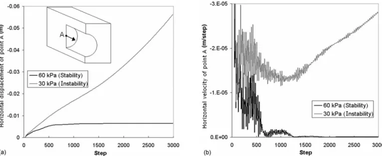
• The initial lower bracket corresponds to any trial pressure for which the system is unstable. This state corresponds to a non-null face extrusion velocity at each point of the tunnel face 关see, for instance, the horizontal velocity of Point A shown in Fig. 2共b兲 where Point A is located at the centre of the tunnel face兴. This nonnull velocity at Point A corresponds to a con-tinuously increasing horizontal displacement at this point, as shown in Fig. 2共a兲, and it means that a steady state of failure or plastic flow is achieved in this case.
• The initial upper bracket corresponds to any trial pressure in which the system is stable. This state corresponds to a zero face extrusion velocity at each point of the tunnel face关see, for instance, the horizontal velocity of Point A shown in Fig. 2共b兲兴. This zero velocity at Point A corresponds to a constant
horizontal displacement at this point as long as the number of cycles increases, as shown in Fig. 2共a兲, and it means that a steady state of static equilibrium is achieved in this case. 2. Next, a new value, midway between the upper and lower
brackets, is tested. If the system is stable for this midway value, the upper bracket is replaced by this new trial pres-sure. If the system does not reach equilibrium, the lower bracket is then replaced by the midway value.
3. Steps 1 and 2 are repeated until the difference between upper and lower brackets is less than a specific tolerance.
The simple bisection method consists of running several cycles for the two states of plastic flow and static equilibrium corresponding, respectively, to the lower and upper brackets. This procedure is very time consuming because the plastic flow state usually occurs after a large number of cycles. This can be dra-matic if one is looking for a precise value of the collapse pressure. A more efficient method called in this paper as “the improved bisection approach” may be used. It allows one to check if the system is unstable much more quickly than the classical ap-proach. This method is similar to that used in FLAC3Dsoftware
for the determination of the safety factor. It may be briefly de-scribed as follows. First, a very high value of the cohesion is affected to the soil. This makes the soil behave as an elastic material. Second, the whole system is set to an unbalanced state by doubling artificially all the values of the internal stresses. The method consists of determining a “representative” number N of cycles. It corresponds to the number of computation cycles that the software must run to return to a static equilibrium state from the previous unbalanced state. This number is generally close to 3,000 steps. When N is determined, the initial value of the cohe-sion is restored. The system is considered in a steady state of plastic flow if it remains unstable after performing these N cycles. As one can easily see, there is no need to run a large number of cycles to check the instability of the system in the improved bi-section method. Interested readers by this method may refer for more details to Fast Lagrangian Analysis of Continua共FLAC3D兲
共1993兲. The improved bisection method was coded in FISH lan-guage into the FLAC3Dsoftware. It allows one to obtain the
col-lapse pressure more quickly than the classical bisection approach.
The CPU time is variable but can be longer than 1 day when using the classical bisection method and becomes equal to 90 min 共on a Core2 Quad CPU 2.40-GHz PC兲 when one uses the im-proved bisection method. Thus, the imim-proved bisection technique is adopted for the computation of the tunnel collapse pressure. Bracketing and bisection are repeated until the difference between the upper and lower brackets becomes smaller than a prescribed tolerance 共e.g., 100 Pa in this paper兲. The tunnel face collapse pressure was found equal to c= 34.5 kPa. The corresponding collapse velocity field given by FLAC3D is provided in Fig. 3.
Stability against collapse is ensured as long as the applied pres-suretis greater than the tunnel collapse pressurec.
SLS: Maximal Settlement
First, it should be emphasized here that the deterministic numeri-cal simulations used in the paper for the SLS are limited to the computation of the ground settlement due to only the applied face pressure. Notice however that the ground settlement is primarily due to the shield tail void. In real shield tunneling cases, the proportion of ground settlement induced by the face pressure may be less than 25% of the total settlement 共cf. Vanoudheusden 2006兲. The settlement due to shield tunneling is pretty much af-fected by the closure of tail void, grouting, unlined length, soil
Fig. 2.共a兲 Horizontal displacement; 共b兲 horizontal velocity of Point A 共center of tunnel face兲 during stability 共static equilibrium兲 and instability
共plastic flow兲
loss, etc., during tunneling. Thus, the present numerical simula-tions can only be regarded as an idealized condition ignoring many important factors concerning tunneling construction. The writers consider the ground settlement due to the sole effect of the face pressure for the following reasons. The face pressure is the parameter that has the most influence on stability. On the other hand, several parameters共among them the face pressure兲 would influence the ground settlement. In this paper, the effect of only one tunneling parameter共i.e., the face pressure兲 on both the sta-bility and deformation analyses of the pressurized shield tunnel-ing was considered in order to be able to make a comparison of the tunnel reliability on both the SLS and ULS due to this unique parameter.
For the computation of the maximal settlement due to an ap-plied pressureton the tunnel face, the excavation by the shield is also modeled here by the stress control method in order to take into account the excavation steps. Contrary to the ULS where the excavation steps were not necessary in the computation procedure of the collapse pressure, in the present SLS, a total of 50 excava-tion steps共with a length of 1 m for each step兲 were performed. Cycling was performed after each excavation step in order to obtain the corresponding displacement. It should be mentioned here that the excavation and the concrete lining installation were applied concurrently. This leads, as mentioned before, to a signifi-cant simplification concerning the simulation of tunneling con-struction and provides the settlement induced by only the face decompression.
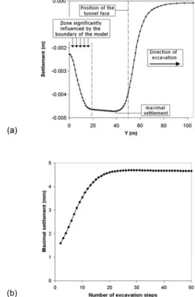
An elastic perfectly plastic model is still used here for the soil since it enables the development of plastic zones that may occur near the tunnel face for the entire range of variation in the applied pressuretand it leads to more accurate solutions than a purely elastic model. A more sophisticated model including nonlinearity in the elastic range would be of interest and may give better results for the settlement. However, it is out of the scope of this paper and will be used in a future research. The numerical simu-lations have shown that the longitudinal limits of the model have a significant influence on the value of the maximal settlement. This is the reason why the mesh used for the assessment of the maximal settlement is much more extended than the previous one along the Y axis. Notice however that the same geometry is adopted here in the X-Z section. The mesh used is presented in Fig. 4. Fig. 5共a兲 shows the settlement along the Y axis after 50 steps of excavation for an applied pressure of 40 kPa. This curve clearly shows the zone, which is significantly influenced by the boundary Y = 0 of the model. The maximal settlement共4.7 mm in this case兲 occurs about 10 m behind the tunnel face. Fig. 5共b兲 presents the maximal settlement versus the number of excavation
steps. This figure shows the stabilization of the maximal settle-ment after about 30 steps of 1 m long. Thus, one can conclude that the 50 steps of excavation adopted in this paper are sufficient to give accurate result for the maximal settlement. Finally, notice that the CPU time required for each computation of the maximal settlement was found to be 130 min on a Core2 Quad CPU 2.40-GHz PC.
Ellipsoid Approach in Reliability Theory
The reliability index of a geotechnical structure is a measure of the safety that takes into account the inherent uncertainties of the input parameters. A widely used reliability index is the Hasofer and Lind共1974兲 index. Its matrix formulation is 共Ditlevsen 1981兲
HL= min
x苸F
冑
共x − x兲TC−1共x − x兲 共1兲in which x = vector representing the n random variables; x = vector of their mean values; and C = their covariance matrix. The minimization of Eq.共1兲 is performed subject to the constraint G共x兲ⱕ0, where the limit state surface G共x兲=0 separates the n-dimensional domain of random variables into two regions: a failure region F represented by G共x兲ⱕ0 and a safe region given by G共x兲⬎0.
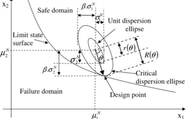
Low and Tang 共1997a, 2004兲 introduced the concept of an expanding ellipsoid 共or ellipse in the two-dimensional case兲, as shown in Fig. 6, and led to a simple method of computing the Hasofer-Lind reliability index in the physical space of the random variables. These writers reported that the Hasofer-Lind reliability indexHLmay be regarded as the codirectional axis ratio of the
smallest ellipsoid that just touches the limit state surface to the
Fig. 4. Soil domain and mesh used in FLAC3Dfor SLS
Fig. 5. Settlement determination in SLS:共a兲 settlement along Y axis
after 50 excavation steps whent= 40 kPa;共b兲 maximal settlement
unit dispersion ellipsoid关i.e., corresponding to HL= 1 in Eq.共1兲
without the min兴. They also stated that finding the smallest ellip-soid that is tangent to the limit state surface is equivalent to find-ing the most probable failure point. When the random variables are nonnormal and correlated, the optimization approach uses the Rackwitz-Fiessler equations to compute the equivalent normal meanxNand the equivalent normal standard deviationxNwithout the need to diagonalize the correlation matrix, as shown in Low and Tang 共2004兲, Low 共2005兲, and Youssef Abdel Massih et al. 共2008兲. Furthermore, the iterative computations of the equivalent normal meanxNand the equivalent normal standard deviationxN for each trial design point are automatic during the constrained optimization search.
In this paper, by the method of Low and Tang, one literally sets up a tilted ellipsoid in Microsoft Excel and uses the solver to minimize the dispersion ellipsoid subject to the constraint that it is tangent to the limit state surface. Eq. 共1兲 may be rewritten as 共Low and Tang 1997b, 2004兲
HL= min x苸F
冑
冋
x −xN x N册
T 关R兴−1冋
x −x N x N册
共2兲in which 关R兴−1= inverse of the correlation matrix. This equation will be used to set up the ellipsoid in Microsoft Excel since the correlation matrix关R兴 displays the correlation structure more ex-plicitly than the covariance matrix关C兴.
From the first order reliability method 共FORM兲 and the Hasofer-Lind reliability indexHL, one can approximate the
fail-ure probability as follows:
Pf⬇ ⌽共− HL兲 共3兲
where⌽共·兲=cumulative distribution function of a standard nor-mal variable. In this method, the limit state function is approxi-mated by a hyperplane tangent to the limit state surface at the design point.
Reliability Analysis of Circular Tunnels
The aim of this paper is to perform a reliability analysis of a circular tunnel driven by a pressurized shield in a c − soil. Two failure or unsatisfactory performance modes are considered in the analysis. The first one involves the ULS and emphasizes on the computation of the tunnel collapse pressure. The second one con-siders the SLS and focuses on the maximal settlement due to the applied face pressure. The two deterministic models presented
above are used. The RSM is employed to find an approximation of the analytically unknown performance functions. Due to the relatively low effect of the elastic modulus E and the Poisson ratio on the tunnel collapse pressure, only c and will be considered as random variables while studying the ULS; the soil dilation angle is taken equal to zero in the present analysis and it is considered as a deterministic parameter. For the study of the SLS, a parametric study is performed here to check the sensitivity of the maximal settlement to the five parameters of the elastoplas-tic Mohr-Coulomb constitutive model共i.e., E, , c, , and 兲. A total of 15 simulations corresponding to three different values of each parameter共see Table 1兲 are studied, as shown in Fig. 7. This study clearly shows that Poisson coefficient and dilatancy angle have almost no effect on the maximal settlement, whereas E, c, and have a significant effect on this settlement. Furthermore, it was shown that small values of c and may lead to instability 共plastic flow兲 of the tunnel face. Consequently, only the random-ness of c,, and E will be taken into consideration in the analysis of the SLS.
For the statistical moments of the random variables, Phoon and Kulhawy 共1999兲 stated from an exhaustive study of cone penetration test and triaxial tests results that the coefficient of variation 共COV兲 of the cohesion could vary from 10 to 55%; Cherubini et al.共1993兲 recommended the interval 12–45% for the stiff clays and a higher limit of 80% for very soft clays. For the COV of the friction angle, Phoon and Kulhawy共1999兲 proposed
Table 1. Fifteen Simulations Considered for the Parametric Study of the
Settlement共for Each Simulation, One Parameter May Take Three Differ-ent Values Including Its Reference Value While the Four Other Param-eters Are Fixed to their Reference Values, i.e., a Total of 5⫻3=15 Simu-lations兲
Variable
E
共MPa兲 共kPa兲c 共degrees兲 共degrees兲 Reference values 240 0.3 7 17 0 Case 1 400 0.45 21 30 10 Case 2 Reference value of E Reference value of Reference value of c Reference value of 5 Case 3 100 0.15 0 12 Reference value of Failure domain Safe domain Limit state surface Design point Critical dispersion ellipse N 2 .σ β N 2 σ N 1 σ Unit dispersion ellipse N 1 µ N 2 µ x1 x2 N 1 .σ β ( )θ r
( )
θ R θFig. 6. Design point and equivalent normal dispersion ellipses in the
space of two random variables
the interval of 5–15%. For the COV of Young’s modulus, the same authors proposed 30%, Bauer and Pula 共2000兲 suggested 15%, and Baecher and Christian 共2003兲 proposed the interval 2–42%. The illustrative values used in this paper for the statistical moments of the shear strength parameters and Young’s modulus belong to the intervals proposed by the above cited authors and are given as follows: c= 7 kPa, = 17°, E= 240 MPa, COVc= 20%, COV= 10%, and COVE= 15%. For the probability distribution of the random variables, two cases may be studied. In the first case, referred to as normal variables, c, , and E are considered as normal variables. In the second case, referred to as nonnormal variables, c and E are assumed to be lognormally dis-tributed while is assumed to be bounded and a beta distribution is used 共Fenton and Griffiths 2003兲. The parameters of the beta distribution are determined from the mean value and standard deviation of 共Haldar and Mahadevan 2000兲. It should be men-tioned that for the ULS for which only the shear strength param-eters are considered as random variables, E will be considered as deterministic with its mean value and with a zero COV. Concern-ing the coefficients of correlation between random variables, only a negative correlation between c and with 共c,= −0.5兲 is as-sumed to exist when these random variables are considered as correlated.
After a brief description of the performance functions used in the present analysis, the RSM and its numerical implementation are presented. Then, the probabilistic numerical results based on this method are presented and discussed.
Performance Functions
Two performance functions are used in the reliability analysis. The first one is defined with respect to the collapse mode of failure in the ULS as follows:
G1=
t
c− 1 共4兲
wheret= applied pressure on the tunnel face andc= tunnel col-lapse pressure computed using FLAC3D. The second performance
function, which is defined in the SLS with respect to a prescribed admissible settlement, is given as follows:
G2=max− 共5兲
where=maximal settlement 共as explained before兲 calculated by FLAC3Ddue to an applied pressuretand
max= maximal
admis-sible prescribed settlement.
Response Surface Method
When using numerical simulations, the closed form solution of the performance function is not available. Thus, the determination of the reliability index is not straightforward. An algorithm based on the RSM proposed by Tandjiria et al. 共2000兲 is used in this paper with the aim to calculate the reliability index and the cor-responding design point. The basic idea of this method is to ap-proximate the performance function by an explicit function of the random variables and to improve the approximation via iterations. The approximate performance function widely used in literature has a quadratic form. It uses a second order polynomial with squared terms. The expression of this approximation is given by
G共x兲 = a0+
兺
i=1 n aixi+兺
i=1 n bixi2 共6兲where xi= random variables; n = number of the random variables; and共ai, bi兲=coefficients to be determined. In this paper, two ran-dom variables c and are considered for the ULS 共i.e., n=2兲. However, n = 3 for the SLS since the random variables used in that case are c,, and E. For both limit states, the random vari-ables are characterized by their mean values iand their COVs i. A brief explanation of the algorithm used is as follows: 1. Evaluate the performance function G共x兲 at the mean value
point and the 2n points each at ⫾k, where k is usually equal to 1 共this parameter may be varied in some cases if necessary兲.
2. The above 2n + 1 values of G共x兲 can be used to solve Eq. 共6兲 for the coefficients共ai, bi兲. This obtains a tentative response surface function.
3. Solve Eq.共1兲 to obtain a tentative design point and a tenta-tiveHLsubject to the constraint that the tentative response
surface function of Step 2 be equal to zero.
4. Repeat Steps 1–3 until convergence. Each time Step 1 is repeated, the 2n + 1 sampled points are centered at the new tentative design point of Step 3.
Notice finally that Steps 2 and 3 were done using the optimization tools in Microsoft Excel. However, Step 1 was performed using deterministic FLAC3Dcalculations.
Numerical Results
ULS
It should be mentioned here that the quadratic approximation given by Eq.共6兲 was used for the computation of the reliability index in the ULS. Fig. 8 shows the evolution of the successive tentative response surfaces in the standard space 共u1, u2兲 for an
applied pressure equal to 70 kPa when the random variables are
Fig. 8. Evolution of the tentative response surface in the 共u1, u2兲
assumed normal and uncorrelated. A convergence criterion on the reliability index was adopted. It considers that convergence is reached when a difference共in absolute value兲 smaller than 10−2
between two successive reliability indexes is achieved. One can notice that this criterion is reached after three to five iterations. Thus, only 15–25 numerical simulations by FLAC3Dwere
neces-sary. The corresponding CPU time required is about 20 ⫻90 min=1,800 min 共i.e., 30 h兲. A value of 3.50 was found for the reliability index in the case of uncorrelated共c,= 0兲 variables and a value of 4.47 for correlated 共c,= −0.5兲 variables. These values correspond to failure probabilities of 2.3⫻10−4 and 4.0
⫻10−6as calculated by FORM approximation.
Fig. 9 shows a comparison between the reliability results
共re-liability index, design point, and failure pattern兲 as given by the present model using RSM and the limit analysis model by Mollon et al. 共2009兲 in the case of uncorrelated normal variables. Al-though FLAC3D and limit analysis give quite close results
con-cerning the collapse pressure, the limit analysis model by Mollon et al.共2009兲 suffers from the fact that only one part of the circular tunnel face共i.e., an inscribed ellipse兲 is involved by failure, the remaining part of this area is at rest. Hence, the aim of using a FLAC3Dmodel is that this model is a more rigorous deterministic
one in which no a priori assumptions are made concerning the shape of the failure mechanism. Notice finally that the collapse pressure at the design point as computed by FLAC3Dis equal to
70.07 kPa. This pressure is to be compared to the target pressure of 70 kPa. Thus, one can consider the RSM algorithm used in this paper as sufficiently accurate for the computation of the reliability index.
Reliability Index and Design Point
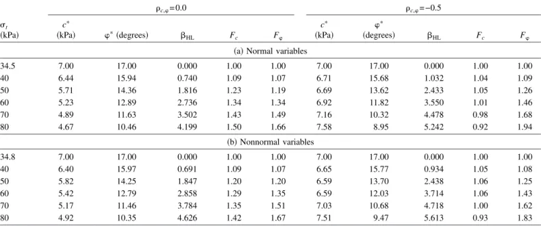
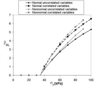
Table 2 presents the Hasofer-Lind reliability index and the corre-sponding design point for different values of the applied pressure t. The cases of normal, nonnormal, correlated 共c,= −0.5兲, and uncorrelated共c,= 0兲 shear strength parameters are considered.
The plot of the reliability index versus the applied pressuret is given in Fig. 10. The reliability index decreases with the de-crease in the applied pressure until it vanishes for an applied pressure equal to the deterministic collapse pressure. This case corresponds to a deterministic state of failure for which t=c using the mean values of the random variables for normal vari-ables共or the equivalent normal mean values for nonnormal vari-ables兲 and the failure probability is equal to 50%. The comparison of the results of correlated variables with those of uncorrelated variables shows that the reliability index corresponding to uncor-related variables is smaller than the one of negatively coruncor-related variables. One can conclude that the hypothesis of uncorrelated shear strength parameters is conservative in comparison to the one of negatively correlated parameters. For instance, when the applied pressure is equal to 60 kPa, the reliability index increases by 30% if the variables c and are considered as negatively correlated. The increase in the reliability index due to a negative
Table 2. Reliability Index and Design Point for ULS for Normal, Nonnormal, Uncorrelated, and Correlated Shear Strength Parameters
t 共kPa兲 c,= 0.0 c,= −0.5 cⴱ 共kPa兲 ⴱ共degrees兲  HL Fc F cⴱ 共kPa兲 ⴱ 共degrees兲 HL Fc F
共a兲 Normal variables
34.5 7.00 17.00 0.000 1.00 1.00 7.00 17.00 0.000 1.00 1.00 40 6.44 15.94 0.740 1.09 1.07 6.71 15.68 1.032 1.04 1.09 50 5.71 14.36 1.816 1.23 1.19 6.69 13.62 2.433 1.05 1.26 60 5.23 12.89 2.736 1.34 1.34 6.92 11.82 3.550 1.01 1.46 70 4.89 11.63 3.502 1.43 1.49 7.16 10.32 4.478 0.98 1.68 80 4.67 10.46 4.199 1.50 1.66 7.58 8.95 5.242 0.92 1.94 共b兲 Nonnormal variables 34.8 7.00 17.00 0.000 1.00 1.00 7.00 17.00 0.000 1.00 1.00 40 6.40 15.97 0.691 1.09 1.07 6.65 15.77 0.934 1.05 1.08 50 5.82 14.25 1.847 1.20 1.20 6.59 13.70 2.438 1.06 1.25 60 5.42 12.79 2.858 1.29 1.35 6.59 12.03 3.714 1.06 1.43 70 5.17 11.46 3.784 1.35 1.51 7.03 10.68 4.718 1.00 1.62 80 4.92 10.35 4.626 1.42 1.67 7.51 9.47 5.613 0.93 1.83
Fig. 9. Comparison of the reliability results and the corresponding
failure pattern as given by the present RSM and the limit analysis
correlation may be explained with the aid of Fig. 11 in which the critical ellipse corresponding to a negative correlation is greater than that of no correlation. The reliability index of nonnormal variables is slightly greater than that of normal variables. For the same pressure of 60 kPa, the reliability index increases by only 5% if the variables are considered as nonnormal. The observation that both normal and nonnormal variables give close results may be explained by the fact that the cumulative distribution functions of normal and nonnormal variables are practically similar in the zone of interest to the engineers corresponding to the different design points obtained in the paper !these curves are not shown in the paper!.
The values of the design points corresponding to different val-ues of the applied pressure can give an idea about the partial safety factors of each of the strength parameters and tan as follows:
⌽= ! 苸7!
⌽ =tan苸 !
tan ! 苸8!
Table 2 shows that for uncorrelated shear strength parameters, the values of ! and ! at the design point are smaller than their
respective mean values and decrease with the increase in the
ap-plied pressure. Consequently, the partial safety factors⌽and⌽ decrease with the decrease in the applied pressure. They tend to 1 when != . For negatively correlated shear strength parameters, ! slightly exceeds the mean for some values of the applied
pres-sure. This can be explained by the counterclockwise rotation of the critical dispersion ellipse due to the negative correlation !cf. Fig. 11!. The position of the design point, which is the point of tangency between the critical ellipse and the limit state surface, changes from the one found for uncorrelated soil shear strength parameters. A higher value of ! and a lower value of ! were
found in the case of negative correlation. Consequently, ! can
become greater than the mean value for a negative correlation. This conclusion is similar to that found by Youssef Abdel Massih and Soubra !2008!.
SLS
The classical RSM used before in the ULS was found not conve-nient in the present case of the SLS. Two issues were encoun-tered:
1. It was impossible to compute a settlement for some sampling points after a given number! of iterations. This is because these cases lead to a collapse of the tunnel face. This oc-curred when calculating the settlement corresponding to points such as 苸!− , !,! !! or 苸!, !− ,! !! for which a smaller value of ! or ! was considered for the settlement computations.
2. It was found that the successive iterations of the RSM do not converge to a design point when using a quadratic approxi-mation for the limit state surface. Another form of this limit state function was necessary as will be seen later.
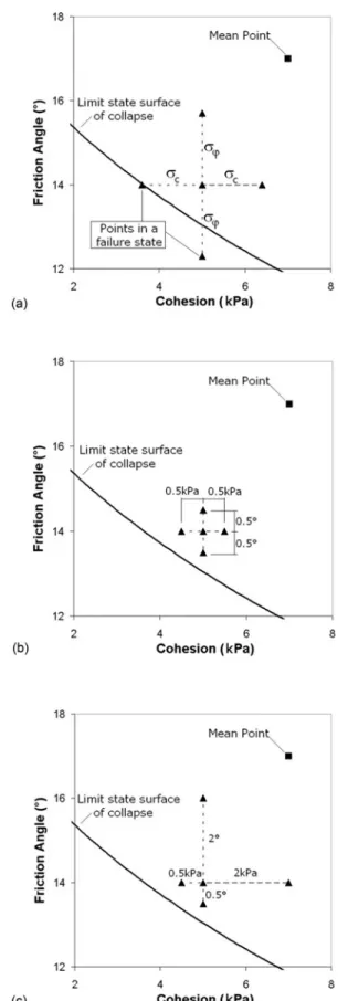
The first issue may be explained with the aid of Fig. 12!a!. This figure shows the seven sampling points projected on a苸, ! plane. Thus, only five points are visible in that figure. It can be easily seen that some sampling points can lead to a collapse of the tunnel face since they correspond to shear strength parameters located in the failure zone of the 苸, ! plane as defined in the ULS study. Two different ways may be used to overcome this issue. The first one consists in reducing the! value defined in the RSM, as shown in Fig. 12!b!. This resolves the collapse issue for all the sampling points but unfortunately it does not lead to con-vergence. This is because the approximation of the limit state surface was not accurate in this case; this surface being based on very neighboring sampling points. A second and more efficient method is proposed in Fig. 12!c! where the shear strength param-eters are chosen in a nonsymmetrical manner with respect to the central point. Thus, the seven sampling points used for the deter-mination of the limit state surface approximation become 苸!, !,! !! , 苸!+ 1.2 , !,! !! , 苸!− 0.3 , !,! !! , 苸!, !+ 1.4 ,! !! ,
苸!, !− 0.3 ,! !! , 苸!, !,! !+ ! ! , and 苸!, !,! !− ! ! . This choice
of the sampling points was made arbitrarily. It prevents the face collapse !by not reducing too much the value of and !. It slightly shifts the sampling points to the safe domain. However, these points remain close to the limit state surface in order to obtain a good approximation of this surface. Notice finally that the choice of the values of! has a small influence on the results. The sampling points can thus be located anywhere in the neigh-borhood of the design point. This method will be used in all subsequent SLS simulations.
The second issue is due to the use of a quadratic approxima-tion for the limit state surface. In the present case of the SLS, this approximation was found not convenient since it does not make
Fig. 10. HLversus applied pressure !
µ ρ
µ
ρ µ
Fig. 11. General layout of the critical dispersion ellipse for different
the RSM iterations converge to the design point. A study of a significant number of FLAC3Dsimulations for several values of c,
, and E has shown that the settlement increases with the de-crease in c,, and E. The numerical simulations have also shown
that an infinite settlement corresponding to the collapse of the tunnel face is obtained when one uses the共c,兲 points of the limit state surface of the ULS. From the ULS study, it can be shown that the critical limit state function defined by Eq. 共4兲 共i.e., G1
= 0兲 can be approximated by the following function:
= ␣1c2+␣2c +␣3 共9兲
where ␣1,␣2, and ␣3are constants. By taking into account the
aforementioned observations concerning the sensitivity of the maximal settlement to the different input parameters 共i.e., c, , and E兲, the following equation is suggested as an approximation for the maximal settlement:
共c,,E兲 ⬇ a1+
a2
− 共a3c2+ a4c + a5兲
+ a6E + a7E2 共10兲
The values of a3, a4, and a5are not equal to the values of␣1,␣2,
and␣3but remain very close. As can be seen from this equation,
the maximal settlement increases with the decrease in c,, and E and is equal to infinity for the 共c,兲 points of the limit state surface in ULS. Eq. 共10兲 is governed by seven constants ai 共i = 1 – 7兲 and needs seven FLAC3D settlement computations to be
defined. The nonsymmetrical pattern presented in Fig. 12共c兲 is used. As the present limit state surface is close to the real one, the convergence to the design point was ensured within three or four RSM iterations. This allows one to get the reliability index with ease for a given applied pressure and for a given prescribed settle-ment. The corresponding CPU time required is about 28 ⫻130 min=3,640 min 共i.e., 60 h兲. As an example, the values of the seven constants corresponding to the best approximation of the limit state surface and the corresponding reliability results are given in Table 3 for the case of normal uncorrelated variables and for an applied pressuret= 70 kPa whenvmax= 5 mm. This table gives also the tentative reliability index and design point at the different iterations. Notice that the maximal settlement at the de-sign point as computed by FLAC3D is equal to 5.01 mm. This
settlement is to be compared to the target settlement of 5 mm. Thus, as in the ULS, one can consider the RSM algorithm used in this paper as sufficiently accurate for the computation of the reli-ability index.
Fig. 13 shows the unit and critical dispersion ellipsoids and the limit state surface for an applied pressure equal to 60 kPa and a prescribed settlement equal to 5 mm in the case of normal uncor-related variables. The critical dispersion ellipsoid is the smallest one that just touches the limit state surface.
Reliability Index and Design Point
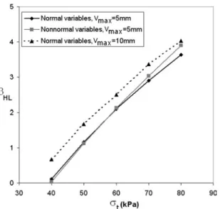
Fig. 14 presents the reliability index of the SLS versus the applied pressuretfor three different cases:
1. Normal variables with a maximal prescribed settlement equal to 5 mm;
2. Nonnormal variables with a maximal prescribed settlement equal to 5 mm; and
3. Normal variables with a maximal prescribed settlement equal to 10 mm.
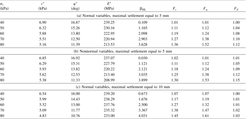
In all these cases, no correlation was considered between the three random variables. The values of the design point and the partial safety factors共Fc, F, and FE兲 are given in Table 4. The same interpretation of the ULS results in terms of the design point and safety factors remain valid in the present case of SLS and thus will not be repeated herein. Fig. 14 shows that 共i兲 the as-sumption of nonnormal variables has almost no effect on the
re-Fig. 12. Different patterns used in SLS共projected on a 共c,兲 plane兲:
共a兲 classic pattern; 共b兲 improved pattern with a reduced k value; and 共c兲 adopted nonsymmetrical pattern
liability index for t⬍60 kPa as in the ULS case and 共ii兲 a prescribed settlement of 10 mm instead of 5 mm increases the reliability index; the increase is equal to 16% whent= 70 kPa.
Comparison between the Two Limit States
Fig. 15 shows a comparison between the values ofHLgiven by
the ULS and the SLS 共in both cases of max= 5 mm and max
= 10 mm兲. The reliability index of both limit states have almost the same evolution versus the applied pressure. This may be ex-plained by the fact that both limit states are controlled by the same parameters 共mainly c and 兲 and correspond to the same physical phenomenon: the occurrence of a settlement can be con-sidered as the beginning of a failure state because it implies plas-tic deformations around the tunnel face. Finally, from Fig. 15, one can easily see that the reliability index against face collapse and the one against a 10-mm maximal settlement are almost the same. Table 5 gives the components and the system reliability index of both limit states. The equations used are given in Youssef Abdel Massih and Soubra共2008兲 and are not repeated herein. The coefficient of correlation between the two limit states was found very close to 1共0.97⬍ULS-SLS⬍1兲 for the different applied pres-sures. This indicates a strong positive correlation between both limit states and confirms the observation made above concerning the evolution of both limit states in the same manner. It was also found that the system reliability index depends on both limit states. It is smaller than the reliability index corresponding to a single failure mode but it is very close to the one of SLS. It is equal to that of SLS for high values of the applied pressure.
Table 3. Design Point along the Different RSM Iterations for SLS共t= 70 kPa andmax= 5 mm兲
RSM iteration number共i兲 Mean point 1 2 3 4
BHLi 0 3.685 2.909 2.897 2.903
ci共kPa兲 7 5.22 5.41 5.58 5.51
i共deg兲 17 11.28 12.65 12.48 12.50
Ei共MPa兲 240 211.05 211.25 220.94 220.94
Best approximation of the limit state surface at the fourth iteration:
a1= 11.67; a2= 5.20; a3= 0.0357; a4= −0.882; a5= 14.75; a6= −0.0684; and a7= 0.000103
Fig. 13. Graphical representation of unit and critical dispersion
el-lipsoids for SLS:共a兲 in the three-dimensional space; 共b兲 projected on
Hence, the contribution of ULS to the system reliability is not significant. As a conclusion, SLS can be used alone for the as-sessment of the tunnel reliability.
Conclusions
A reliability-based analysis of a shallow circular tunnel driven by a pressurized shield in a c − soil is presented. Both the ULS and the SLS are considered in the analysis. Two deterministic models based on numerical simulations using the Lagrangian explicit finite-difference code FLAC3Dare employed. The first one
com-putes the collapse pressure of the tunnel face and the second one calculates the maximal settlement due to a given applied pressure on the tunnel face. In both models, the stress control method is
used. Concerning the assessment of the tunnel reliability, the Hasofer-Lind reliability index is adopted here. The RSM is used to find an approximation of the analytically unknown limit state surfaces and the corresponding reliability indices. Only the soil shear strength parameters are considered as random variables while studying the ULS. However, the randomness of both Young’s modulus and the shear strength parameters of the soil is taken into account in the SLS. The main conclusions of this paper can be summarized as follows.
For the ULS, the hypothesis of uncorrelated shear strength parameters was found conservative in comparison to the one of negatively correlated variables. For uncorrelated shear strength parameters, the values of cⴱandⴱat the design point are found smaller than their respective mean values and increase with the decrease in the applied pressure t. Consequently, the partial safety factors Fcand Fdecrease with the decrease in the applied
pressure. They tend to 1 when t=c. For negatively correlated shear strength parameters, cⴱslightly exceeds the mean for some values of the applied pressure.
For the SLS, when the shear strength parameters are consid-ered as uncorrelated, the partial safety factors Fc, F, and FE decrease with the decrease int. They tend to 1 whentis equal to the pressure that leads to the maximal prescribed settlement maxfor the mean values of c,, and E.
For both ULS and SLS, the assumption of nonnormal
distri-Table 4. Reliability Index and Design Point for SLS for Normal and Nonnormal Variables with No Correlation
t 共kPa兲 c ⴱ 共kPa兲 ⴱ 共deg兲 E ⴱ 共MPa兲 HL Fc F FE
共a兲 Normal variables, maximal settlement equal to 5 mm
40 6.90 16.87 239.25 0.109 1.01 1.01 1.00
50 6.32 15.26 230.16 1.165 1.11 1.12 1.04
60 5.88 13.80 222.95 2.098 1.19 1.24 1.08
70 5.51 12.50 220.94 2.903 1.27 1.38 1.10
80 5.16 11.39 213.53 3.628 1.36 1.52 1.12
共b兲 Nonnormal variables, maximal settlement equal to 5 mm
40 6.85 16.92 237.07 0.030 1.02 1.01 1.01
50 6.29 15.31 227.79 1.121 1.11 1.12 1.05
60 5.93 13.82 220.22 2.121 1.18 1.24 1.09
70 5.62 12.53 213.40 3.035 1.25 1.38 1.12
80 5.38 11.33 208.99 3.899 1.30 1.53 1.15
共c兲 Normal variables, maximal settlement equal to 10 mm
40 6.54 16.00 239.20 0.673 1.07 1.07 1.00
50 5.99 14.43 238.29 1.676 1.17 1.19 1.01
60 5.52 13.00 237.76 2.500 1.27 1.32 1.01
70 5.09 11.77 235.32 3.367 1.38 1.47 1.02
80 4.83 10.76 233.00 4.031 1.45 1.61 1.03
Table 5. Reliability Index of the System ULS-SLS formax= 5 mm
t 共kPa兲 HL ULS SLS System ULS-SLS 40 0.740 0.109 0.089 50 1.806 1.165 1.163 60 2.726 2.098 2.097 70 3.502 2.901 2.901 80 4.189 3.628 3.628
bution for the random variables has almost no effect on the reli-ability index for the practical range of values of the applied pressure t. The reliability index of both limit states follows the same evolution with the increase in the applied pressure. This may be explained by the fact that both limit states are controlled by the same parameters共mainly c and 兲 and correspond to the same physical phenomenon: the occurrence of a settlement can be considered as the beginning of a failure state because it implies plastic deformations around the tunnel face.
It was found that the system reliability index depends on both limit states. It is smaller than the reliability index corresponding to a single failure mode but it is very close to the one of SLS. It is equal to that of SLS for high values of the applied pressure. Hence, the contribution of ULS to the system reliability is not significant. As a conclusion, SLS can be used alone for the as-sessment of the tunnel reliability. It should be remembered here that SLS in the present paper is based on the computation of the settlement due to only the face pressure. In a future work, it is suggested to investigate a more sophisticated SLS deterministic model that considers an exhaustive analysis of the total settlement due to the different construction parameters and to perform a probabilistic analysis based on this unique limit state. The new probabilistic SLS model can take advantage of the thorough analysis concerning共1兲 the shape of the response surface found in the paper; and 共2兲 the nonsymmetrical pattern of the sampling points since the influence of both c and on the settlement is expected to remain the same in the new sophisticated determinis-tic model.
References
Baecher, G. B., and Christian, J. T. 共2003兲. Reliability and statistics in
geotechnical engineering, Wiley.
Bauer, J., and Pula, W. 共2000兲. “Reliability with respect to settlement limit-states of shallow foundations on linearly-deformable subsoil.”
Comput. Geotech., 26共1兲, 281–308.
Cherubini, C., Giasi, I., and Rethati, L.共1993兲. “The coefficient of varia-tion of some geotechnical parameters.” Probabilistic methods in
geo-technical engineering, K. S. Li and S.-C. R. Lo, eds., Balkema,
Rotterdam, 179–183.
Dias, D., and Kastner, R.共2005兲. “Modélisation numérique de l’apport du renforcement par boulonnage du front de taille des tunnels.” Can.
Geotech. J., 42, 1656–1674共in French兲.
Dias, D., Kastner, R., and Dubois, P.共1997兲. “Tunnel face reinforcement by bolting: Strain approach using 3D analysis.” Proc., Int. Conf. on
Tunneling under Difficult Conditions, Basel, Switzerland, Balkema,
Rotterdam.
Dias, D., Kastner, R., and Jassionnesse, C. 共2002兲. “Sols renforcés par boulonnage. Etude numérique et application au front de taille d’un tunnel profond.” Geotechnique, 52共1兲, 15–27 共in French兲.
Ditlevsen, O.共1981兲. Uncertainty modeling: With applications to
multi-dimensional civil engineering systems, McGraw-Hill, New York.
Eclaircy-Caudron, S., Dias, D., and Kastner, R.共2007兲. “Inverse analysis on measurements realized during a tunnel excavation.” Proc.,
ITA-AITES World Tunnel Congress 2007, Prague, Czech Republic, Barták
et al., eds.
Fenton, G. A., and Griffiths, D. V.共2003兲. “Bearing capacity prediction of spatially random C − soils.” Can. Geotech. J., 40, 54–65. FLAC3D.共1993兲. Fast Lagrangian analysis of continua, ITASCA
Con-sulting Group, Inc., Minneapolis.
Haldar, A., and Mahadevan, S.共2000兲. Probability, reliability, and
statis-tical methods in engineering design, Wiley, New York.
Hasofer, A. M., and Lind, N. C. 共1974兲. “Exact and invariant second-moment code format.” J. Engrg. Mech. Div., 100共1兲, 111–121. Jardine, R. J., Potts, D. M., Fourie, A. B., and Burland, J. B.共1986兲.
“Studies of the influence of nonlinear stress strain characteristics in soil-structure interaction.” Geotechnique, 36共3兲, 377–396.
Jenck, O., and Dias, D.共2003兲. “Numerical analysis of the volume loss influence on building during tunnel excavation.” Proc., 3rd Int. FLAC
Symp.—FLAC and FLAC3D Numerical Modeling in Geomechanics,
Sudbury, Ontario, Canada, C. Detournay and R. Hart, eds.
Jenck, O., and Dias, D.共2004兲. “Analyse tridimensionnelle en différences finies de l’interaction entre une structure en béton et le creusement d’un tunnel à faible profondeur.” Geotechnique, 54共8兲, 519–528 共in French兲.
Low, B. K.共2005兲. “Reliability-based design applied to retaining walls.”
Geotechnique, 55共1兲, 63–75.
Low, B. K., and Tang, W. H. 共1997a兲. “Efficient reliability evaluation using spreadsheet.” J. Eng. Mech., 123共7兲, 749–752.
Low, B. K., and Tang, W. H.共1997b兲. “Reliability analysis of reinforced embankments on soft ground.” Can. Geotech. J., 34, 672–685. Low, B. K., and Tang, W. H.共2004兲. “Reliability analysis using
object-oriented constrained optimization.” Struct. Safety, 26, 69–89. Mollon, G., Dias, D., and Soubra, A.-H. 共2009兲. “Probabilistic analysis
and design of circular tunnels against face stability.” Int. J. Geomech., in press.
Mroueh, H., and Shahrour, I.共2003兲. “A full 3-D finite element analysis of tunneling-adjacent structures interaction.” Computers and
Geotech-nics, 30, 245–253.
Phoon, K.-K., and Kulhawy, F. H.共1999兲. “Evaluation of geotechnical property variablity.” Can. Geotech. J., 36, 625–639.
Potts, D. M., and Addenbrooke, T. I.共1997兲. “A structure’s influence on tunneling induced ground movements.” Geotech. Eng., 125共2兲, 109– 125.
Ribeiro e Sousa, L., Dias, D., and Barreto, J. 共2003兲. “Lisbon metro yellow line extension. Structural behavior of the Ameixoeira station.”
Proc., 12th Panamerican Conf. on Soil Mechanics and Geotechnical Engineering, Boston, Verlag Glückauf Gmbh, eds.
Tandjiria, V., Teh, C. I., and Low, B. K.共2000兲. “Reliability analysis of laterally loaded piles using response surface methods.” Struct. Safety,
22, 335–355.
Vanoudheusden, E.共2006兲. “Impact de la construction de tunnels urbains sur les mouvements de sol et le bâti existant—Incidence du mode de pressurisation du front.” Ph.D. thesis, INSA Lyon, Lyon, France共in French兲.
Wong, H., Subrin, D., and Dias, D.共2006兲. “Convergence-confinement analysis of a bolt-supported tunnel using homogenization method.”
Can. Geotech. J., 43共5兲, 462–483.
Yoo, C. S.共2002兲. “Finite-element analysis of tunnel face reinforced by longitudinal pipes.” Computers and Geotechnics, 29共1兲, 73–94. Youssef Abdel Massih, D. S., and Soubra, A.-H. 共2008兲.
“Reliability-based analysis of strip footings using response surface methodology.”
Int. J. Geomech., 8共2兲, 134–143.
Youssef Abdel Massih, D. S., Soubra, A.-H., and Low, B. K. 共2008兲. “Reliability-based analysis and design of strip footings against bear-ing capacity failure.” J. Geotech. Geoenviron. Eng., 134共7兲, 917–928.