HAL Id: hal-01703248
https://hal.archives-ouvertes.fr/hal-01703248
Submitted on 5 Mar 2019
HAL is a multi-disciplinary open access
archive for the deposit and dissemination of
sci-entific research documents, whether they are
pub-lished or not. The documents may come from
teaching and research institutions in France or
abroad, or from public or private research centers.
L’archive ouverte pluridisciplinaire HAL, est
destinée au dépôt et à la diffusion de documents
scientifiques de niveau recherche, publiés ou non,
émanant des établissements d’enseignement et de
recherche français ou étrangers, des laboratoires
publics ou privés.
Simulation of the two stages stretch-blow molding
process: Infrared heating and blowing modeling
Maxime Bordival, Fabrice Schmidt, Yannick Le Maoult, Vincent Velay
To cite this version:
Maxime Bordival, Fabrice Schmidt, Yannick Le Maoult, Vincent Velay. Simulation of the two stages
stretch-blow molding process: Infrared heating and blowing modeling. NUMIFORM 2007 - 9th
Inter-national conference on numerical methods in industrial forming processes, Jun 2007, Porto, Portugal.
pp.519+. �hal-01703248�
Simulation of the Two Stages Stretch-Blow Molding
Process: Infrared Heating and Blowing Modeling
M. Bordival, F.M. Schmidt, Y. Le Maoult, V. Velay
CROMeP - Ecole des Mines d’Albi Carmaux - Campus Jarlard - 81013 Albi cedex 09 - France Abstract. In the Stretch-Blow Molding (SBM) process, the temperature distribution of the reheated perform affects drastically the blowing kinematic, the bottle thickness distribution, as well as the orientation induced by stretching. Consequently, mechanical and optical properties of the final bottle are closely related to heating conditions. In order to predict the 3D temperature distribution of a rotating preform, numerical software using control-volume method has been developed. Since PET behaves like a semi-transparent medium, the radiative flux absorption was computed using Beer Lambert law. In a second step, 2D axi-symmetric simulations of the SBM have been developed using the finite element package ABAQUS®. Temperature profiles through the preform wall thickness and along its length were computed and applied as initial condition. Air pressure inside the preform was not considered as an input variable, but was automatically computed using a thermodynamic model. The heat transfer coefficient applied between the mold and the polymer was also measured. Finally, the G’sell law was used for modeling PET behavior. For both heating and blowing stage simulations, a good agreement has been observed with experimental measurements. This work is part of the European project "APT_PACK" (Advanced knowledge of Polymer deformation for Tomorrow’s PACKaging). Keywords: Stretch-blow molding process (SBM), heat transfer modeling, blowing simulation, G’sell law. PACS: 44.05.+e; 44.40.+a; 83.60.St;
INTRODUCTION
In a typical Stretch-Bow Molding (SBM) process, a Polyethylene Terephthalate (PET) preform is heated in an infrared (IR) oven to its forming temperature (around 100°C), and brought into contact with a mold of the desired shape. In such a process, the quality of the final bottle is closely related to heating conditions. Indeed, the preform temperature distribution has a strong effect on the blowing kinematic (stretching and inflation), and consequently on the thickness distribution of the final part. Temperature also affects the orientation induced by stretching, which, in turn, affects mechanical and optical properties of the bottle [1]. Temperature is therefore one of the most important parameters in SBM. However, its measurement remains a delicate task, especially in the thickness direction. Some experimental methods, such as IR thermography allows to measure the surface temperature during heating, but not its profile through the material thickness [2]. Recently the use of thermocouples inserted in the preform thickness was investigated in [3]. On the other hand, numerical methods are increasingly used. Researchers implemented models into commercial finite-element packages like ANSYS® [4], FORGE3® [5], or
developed their own software [6-8] with the aim of predicting the three-dimensional temperature distribution in the preform. Finally, some studies focused on the development of numerical optimization strategies for the SBM. Automatic preform shape optimization was proposed in [9], while optimization of heating system design was investigated in [10]. The objective was to target a uniform temperature profile along the preform length.
The simulation of the blowing step has been also the subject of significant researches within the last two decades. Few studies focused on the feasibility of 3D temperature-displacement simulations [5, 11]. But on the whole, researchers proposed 2D axi-symmetric models, with different material laws. A review is proposed in [5]. It can be noticed that the air pressure inside the preform is generally applied as a boundary condition, which can lead to unrealistic results [12]. Moreover, temperature distribution through the preform wall thickness is generally omitted.
In this work, a simulation of the two stage SBM process is proposed. The 3D temperature distribution of a rotating preform was computed taking into account all the process conditions, and the real oven design. In a second step, this temperature distribution (particularly through the wall thickness) was applied
as initial condition for the simulation of the blowing step. For that, the finite element commercial package ABAQUS® was used. Thanks to a thermodynamic model, the air pressure inside the preform is automatically calculated during simulation. Following sections focus on presenting each model.
PREFORM HEATING MODELING
In the SBM process, heating devices are often composed by a set of halogen lamps associated to aluminum reflectors. The preform translates through the oven, and is animated by a rotational movement to provide a uniform temperature along its circumference. Radiation emitted by the IR lamps is partially absorbed through the preform thickness, before being diffused in each space direction. Additionally, the preform tends to be cooled by air venting. In other words, preform reheating results from a combination between conductive, convective, and radiative heat transfers.
Heat Balance Equation
The evolution versus time of the preform temperature is governed by the following heat balance equation:
(
)
r p k T q dt dT c =∇⋅ ∇ −∇⋅ ρ (1)Where T = temperature, t = time, ρ = density, cp =
specific heat, k = thermal conductivity, qr = radiative
heat flux density. In order to solve this equation in 3D, a finite volume discretization is adopted. For that, the preform is meshed into hexahedral elements called control volumes. Equation (1) is integrated over each control volume and over the time, to obtain the following integro-differential formulation:
(
)
(
q n)
d dt dt d n T k dt d t T c t r t t p Γ − Γ ∇ = Ω ∂ ∂∫∫
∫∫
∫ ∫
∆ Γ ∆ Γ ∆ Ω . . ρ (2)where Ω = control volume, Γ = surface of a control volume. Unknown temperatures are computed at the cell centre of each element. While the internal side of the preform is supposed to be adiabatic, the following boundary condition is applied to the external one:
(
)
(
4 4)
∞ ∞ + − − = ∂ ∂ − h T T T T n T k c P PET P P σ ε (3)Where hc = natural heat transfer coefficient, εPET =
PET mean emissivity, σ = Stefan-Boltzman constant, Tp = preform surface temperature at external side, T∞ =
ambient temperature. The method used for estimating PET mean emissivity is fully detailed in [2]. This boundary condition takes into account two types of thermal exchanges. The first one is due to the cooling by natural convection, the second one to the own emission of the preform. These exchanges are particularly important during the cooling stage.
Radiative Transfer Modeling
Over the spectral band corresponding to the IR lamps emission (0.38-10µm), PET behaves like a semi-transparent body. This involves that the radiative heat flux is absorbed inside the wall thickness of the preform, and can not be simply applied as a boundary condition. The radiation absorption must be taken into account through the divergence of the radiative heat flux, previously presented in the heat balance equation. This term represents the amount of radiative energy absorbed per volume unit; it is also more commonly called radiative source term. The computation of this source term can not be carried out without a precise understanding of radiative transfer properties, including its spectral and directional dependencies. Researchers proposed different numerical methods in order to compute the radiative source term, like raytracing [5] or zonal method [6]. The method used in this work is divided into two steps:
First of all, radiative heat fluxes reaching the preform surface are computed. For that, IR lamps are meshed into surface elements of which the contribution is taken into account via view factors computation. Moreover, IR lamps are assumed to behave like isothermal grey-bodies. Their emission is then defined by the Planck’s law [13]. Finally, incident fluxes are calculated with the following equation:
(
)
(
)
t( )
ti i i ipS L T F qλ0= 1−ρλ∑
ελπ λ (4)Where ρλ = PET reflexion coefficient, Fip = view
factor between the lamp element i and the preform, Si
= surface area of the lamp element, εtλ = tungsten
emissivity, Lλ = Planck’s intensity of the lamp i at the
filament temperature Tti.
In a second time, the radiation absorption is computed according to the Beer-Lambert law (under the assumption of the non-scattering cold medium [13]):
( )
x q(
x)
Where qλ(x) = spectral radiative heat flux density at
the location x, qλ0 = incident spectral radiative heat
flux density, κλ = PET spectral absorption coefficient
(in m-1).
Finally, the radiative source term is computed according to the following equation:
( )
κ κλ λ λ λ λq e d x qr − x ∆∫
− = ⋅ ∇ 0 (6)Application - Results and Discussion
Software previously presented was used to simulate the reheating of a rotating preform with the processing conditions used on the laboratory blowing machine. The oven is composed of six halogen lamps (1 kW power), with ceramic and back aluminum reflectors. After 50 s heating, the preform is cooled down by natural convection during 10 s. The natural convection coefficient was calculated using the empirical correlation of Churchill and Chu [14]. Its value was estimated to 7 W.m-2.K-1. Percentages of nominal power of each lamp are reported TABLE 1. The preform rotating speed is equal to 1.2 rps.
TABLE 1. Process parameters of the IR oven P1 (%) P2 (%) P3 (%) P4 (%) P5 (%) P6 (%) theat (s) tcool (s) 100 100 18 5 50 100 50 10
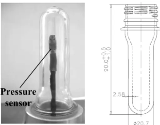
The preform used is 18.5 g weight, 2.58 mm thickness. The Material is PET TF9 grade (IV=0.74). An illustration is displayed FIGURE 1.
FIGURE 1. 18.5 g preform – PET T74F9 (IV=0.74).
Temperature measurements were performed in order to validate simulations. As it was demonstrated in [2], PET behaves like an opaque body over the 8-12 µm spectral band. For this reason, an AGEMA 880 LW IR camera, functioning within the long wave spectral band 8-12 µm, has been chosen. This choice
makes possible to affirm that the camera measures a surface temperature. PET mean emissivity was also measured by following the protocol fully detailed in [2]. Its value is equal to 0.93.
FIGURE 2 illustrates the external temperature distribution computed with the IR heating software, as well as the measured temperature cartography.
FIGURE 2. External temperature distribution after cooling – A: measured – B: simulated.
In the aim of achieving more precise comparisons, the temperature profile along the preform length (at the end of the cooling step) is represented FIGURE 3. A good agreement between simulations and measurements can be observed, since the global error is less than 10%.
FIGURE 3. External temperature profile along the preform length after 10 s cooling.
FIGURE 4 illustrates the variation of temperature versus time on a single point, located at 47 mm from the neck of the preform (this point was chosen because it corresponds to the node located at the middle height of the mesh). This curve shows clearly the effect of the cooling stage. Indeed, it is interesting to notice that after 3 s of cooling (also called inversion time), temperature on internal side becomes higher than on the external one. This phenomenon can be easily Pressure
sensor
explained: while natural convection tends to cool the external side, the internal one is heated by heat conduction. In the SBM process, this point remains crucial. Indeed, there can be a significant difference between the inside and outside hoop stretch ratios. In order to ensure a good uniformity of the stress distribution through the thickness of the bottle, it is necessary to deliberately develop a non-uniform temperature profile throughout the preform before stretch and blowing.
FIGURE 4. Variation of temperature versus time.
Finally, FIGURE 5 shows clearly that the temperature distribution through the thickness is not linear, but exponential. It can be seen that the temperature difference is around 4°C at the end of the thermal conditioning step. This value is of course strongly related to the cooling conditions.
FIGURE 5. Temperature profiles through the preform wall thickness. Same location as FIGURE 4.
As a conclusion, results demonstrated the efficiency of the model developed in CROMeP. Infrared heating software remains a robust tool, allowing a better understanding of the effect of process parameters on temperature profiles, particularly through the preform wall thickness. It could also be used in order to optimize heating systems [10]. However, a precise understanding of the effect of
temperature on the blowing stage is necessary. For that, numerical model devoted to the simulation of the blowing stage was developed. Following section focuses on giving the key points about this model.
BLOW-MOLDING SIMULATION
Simulations of the SBM process were developed using the commercial finite element package ABAQUS®. In this study, the objective is to simulate the process within the same conditions as on the CROMeP blowing machine, which means: simple mold for 50 cl water bottle and no stretch rod. A special attention was given to the measurement of each initial and boundary condition, namely temperature, air pressure, and heat transfer coefficient between the preform and the mold.
Boundary Conditions
As it was mentioned previously, the preform temperature distribution was measured and calculated in order to be applied as initial condition.
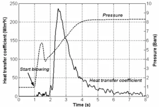
The heat transfer coefficient between the polymer and the mold was measured using a sensor developed for this study. Its peak value was estimated to 230 W.m-2.K-1, as illustrated FIGURE 6. The method used for this measurement is fully detailed in [15]. This coefficient is of prime interest since it affects drastically the cooling time of the plastic bottle.
FIGURE 6. Heat transfer coefficient and air pressure.
Variation versus time of the air pressure inside the preform was measured using a Kulite sensor (FIGURE 1). As illustrated FIGURE 6, the air pressure follows typical variations. In the first time, the pressure increases sharply. As soon as the pressure is sufficient to blow the preform, air volume inside the bottle increases and consequently the pressure drops. While preform internal volume remains constant, the pressure reaches gradually its nominal value. This typical evolution of air pressure gives a good representation of 47 mm
the blowing kinematic. G. Menary [12] has shown that it is unrealistic to apply the pressure directly as a boundary condition. Indeed, the pressure drop would conduct to a deflation of the preform, and not to the rapid inflation observed experimentally. In this study, air pressure is not considered as an input variable, but is automatically computed thanks to the thermodynamic model “fluid element” available in ABAQUS®. This model is based on the perfect gas law. Pressure measurements are only used for validating simulations.
Material Behavior
PET behavior was modeled with the following visco-plastic G’sell material model [16]:
(
)
(
)
( )
− − = + − − = t t a t m T T F with h T W F T k K 1 exp sinh exp exp 1 exp 2 1 0 ε β ε β ε σ & (7)Where
σ
= equivalent Cauchy stress,ε
&
= equivalent strain rate,ε
= cumulated strain, m = sensitivity to strain rate, (K,k0) = consistence. Thismodel takes into account both temperature and strain rate dependencies, as well as the strain hardening which appears for large deformations. It presents the advantage to be numerically stable and relatively easy to implement. However this phenomenological behavior law is reserved to a small range of temperature and strain rate. Moreover, it does not take into account the viscoelasticity of the material. Constitutive parameters have been identified using an inverse method (non-linear constrain algorithm called Sequential Quadratic Programming) from equi-biaxial tensile tests performed in Queen University of Belfast. The thermo-dependency was identified by [16] from shear tests on PET T74F9. This model has been implemented within ABAQUS® via a Fortran subroutine known as user creep.
Blow Molding FEM Model
In order to avoid long computation times, an axi-symmetric model has been chosen. This approach is possible since both preform and mold designs are axi-symmetric, as well as kinematic boundary conditions. The preform was meshed into 46 quadratic shell elements (96 nodes), with five integration points through its thickness in order to take into account the
temperature gradient. The mold used is a prototype developed at CROMeP. It produces 50 cl bottle. This one has been assumed to be rigid and isothermal. Indeed, for one SBM cycle, its temperature increase is about 1°C [14]. In order to compute the heat transfer between the polymer and the mold, a coupled temperature-displacement model was chosen in ABAQUS® Standard (implicit time integration scheme). The viscous dissipation was not calculated. However it could have an important effect on the preform temperature, and consequently on the blowing kinematic. As mentioned previously, no stretch rod is modeled. Finally, the contact between the preform and the mold is assumed to be stick.
Results and Discussion
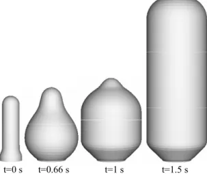
FIGURE 7 illustrates the intermediate preform shapes versus time.
FIGURE 7. Simulation of the preform shape evolution.
Measurements of the thickness distribution of the final part were performed on bottles forming on the CROMeP blowing machine. Comparison with simulation results are illustrated FIGURE 8.
FIGURE 8. Wall thickness distribution of the bottle. t=0 s t=0.66 s t=1 s t=1.5 s
Botton Neck
A good agreement is observed (around 15 % error on the mean thickness). We can notice that the measured thickness distribution is probably not optimal from an industrial point of view. This is due to the preform design used in this study, which is probably not adapted to this type of bottle shape.
Thanks to the thermodynamic model used in this study, it is possible to compare numerical and experimental blowing kinematics, by comparing the evolution of air pressure.
It can be seen FIGURE 9 that the pressure computed by the numerical model is not exactly the same as the measured one. However, tendencies are respected.
FIGURE 9. Computed and measured air pressure.
FUTURE WORK
Future work will aim to consolidate the model presented in this study. It is well known that PET behavior remains the key point for improving the model. Since the pressure curve gives a good representation of the blowing kinematic, it could be envisaged to couple the model to an optimization algorithm in order to identify automatically the constitutive parameters of the material law, by minimizing the difference between the measured pressure, and the calculated one. It is also crucial to investigate the influence of temperature distribution through the preform thickness on the blowing kinematic and on the thickness distribution of the final bottle. A sensitivity study can also be envisaged concerning the heat transfer coefficient mold/polymer, in order to prove its effect on the blowing.
ACKNOWLEDGMENTS
This study was conducted within the frame of 6th EEC framework. STREP project APT_pack; NMP – PRIORITY 3. www.apt-pack.com. Special thanks to Logoplaste Technology for manufacturing the preforms and Tergal Fibre for supplying the material, and QUB for giving tensile test results. Authors thank also V. Lucin for its contribution to this work.
REFERENCES
1. G. Venkateswaran and al, Advances in Polymer Technology 17, 237-249 (1998).
2. S. Monteix and al, QIRT Journal 1, 133-149 (2004). 3. H.-X. Huang and al, Polymer Testing 25, 839-845 (2006). 4. H.-X. Huang and al, SPE ANTEC Tech Papers 12 (2005). 5. C. Champin and al, SPE ANTEC Tech Papers 51 (2005). 6. W. Michaeli and al, SPE ANTEC Tech Papers 30 (2004). 7. S. Monteix and al, Journal of Materials Processing
Technology 119, 90-97 (2001).
8. L. Martin and al, Proceedings of ANTEC, New York, 1999, pp. 982-987.
9. F. Thibault and al, SPE ANTEC Tech Papers 16 (2005). 10. M. Bordival and al, 9th ESAFORM conference on
material forming, Glasgow (UK), 2006, pp. 511-514. 11. S. Wang and al, International Journal for Numerical
Methods in Engineering 48, 501-521 (2000).
12. G. Menary and al, 10th ESAFORM conference on material forming, Zaragoza (Spain), 2007.
13. M. Modest, Radiative Heat Transfer, McGraw-Hill, Inc (1993).
14. F. P. Incropera, Fundamentals of Heat and Mass Transfer, John Wiley & Sons, p 546.
15. M. Bordival and al, 10th ESAFORM conference on material forming, Zaragoza (Spain), 2007.
16. E. Gorlier, "Caractérisation rhéologique et structurale d'un PET. Application au procédé de bi-étirage soufflage de bouteilles", Ph.D. Thesis, ENSMP, 2001.