Memory Analysis and Optimized Allocation of Dataflow Applications on Shared-Memory MPSoCs

HAL Id: hal-01083576

https://hal.archives-ouvertes.fr/hal-01083576v2

Submitted on 10 Dec 2014

HAL is a multi-disciplinary open access

archive for the deposit and dissemination of

sci-entific research documents, whether they are

pub-lished or not. The documents may come from

teaching and research institutions in France or

abroad, or from public or private research centers.

L’archive ouverte pluridisciplinaire HAL, est

destinée au dépôt et à la diffusion de documents

scientifiques de niveau recherche, publiés ou non,

émanant des établissements d’enseignement et de

recherche français ou étrangers, des laboratoires

publics ou privés.

Memory Analysis and Optimized Allocation of Dataflow

Applications on Shared-Memory MPSoCs

Karol Desnos, Maxime Pelcat, Jean-François Nezan, Slaheddine Aridhi

To cite this version:

Karol Desnos, Maxime Pelcat, Jean-François Nezan, Slaheddine Aridhi. Memory Analysis and

Opti-mized Allocation of Dataflow Applications on Shared-Memory MPSoCs: In-Depth Study of a

Com-puter Vision Application. Journal of Signal Processing Systems, Springer, 2015, 80 (1), pp.19-37.

�10.1007/s11265-014-0952-6�. �hal-01083576v2�

(will be inserted by the editor)

Memory Analysis and Optimized Allocation of Dataflow

Applications on Shared-Memory MPSoCs

In-Depth Study of a Computer Vision Application

Jean-Fran¸cois Nezan · Slaheddine Aridhi

Received: date / Accepted: date

Abstract The majority of applications, ranging from the low complexity to very multifaceted entities requir-ing dedicated hardware accelerators, are very well sui-ted for Multiprocessor Systems-on-Chips (MPSoCs). It is critical to understand the general characteristics of a given embedded application: its behavior and its re-quirements in terms of MPSoC resources.

This paper presents a complete method to study the important aspect of memory characteristic of an appli-cation. This method spans the theoretical, architecture-independent memory characterization to the quasi opti-mal static memory allocation of an application on a real shared-memory MPSoC. The application is modeled as an Synchronous Dataflow (SDF) graph which is used to derive a Memory Exclusion Graph (MEG) essential for the analysis and allocation techniques. Practical consid-erations, such as cache coherence and memory broad-casting, are extensively treated.

Memory footprint optimization is demonstrated us-ing the example of a stereo matchus-ing algorithm from the computer vision domain. Experimental results show a reduction of the memory footprint by up to 43% com-pared to a state-of-the-art minimization technique, a throughput improvement of 33% over dynamic alloca-tion, and the introduction of a tradeoff between multi-core scheduling flexibility and memory footprint. Keywords memory allocation · multiprocessor system-on-chip · stereo vision · synchronous dataflow

K. Desnos, M. Pelcat, J.-F. Nezan

IETR, INSA Rennes, UMR CNRS 6164, UEB 20 Avenue des Buttes de Co¨esmes, Rennes E-mail: kdesnos, mpelcat, jnezan@insa-rennes.fr S. Aridhi

Texas Instrument France

Avenue Jack Kilby, Villeneuve Loubet E-mail: saridhi@ti.com

1 Introduction

Over the last decade, the popularity of data-intensive computer vision applications has rapidly grown. Re-search in computer vision traditionally aims at accel-erating execution of vision algorithms with Desktop Graphics Processing Units (GPUs) or hardware imple-mentations. The recent advances in computing power of embedded processors have made embedded systems promising targets for computer vision applications. No-wadays, computer vision is used in a wide variety of applications, ranging from driver assistance [1], to in-dustrial control systems [20], and handheld augmented reality [34]. When developing data-intensive computer vision applications for embedded systems, addressing the memory challenges is an essential task as it can dramatically impact the performance of a system.

Indeed, the identification of the “memory wall” pro-blem in 1995 [35] revealed memory issues as a major concern for developers of embedded systems. Memory issues strongly impact the quality and performance of an embedded system, as the area occupied by the mem-ory can be as large as 80% of a chip and may be respon-sible for a major part of its power consumption [35, 14]. Despite the large silicon area allocated to mem-ory banks, the amount of internal memmem-ory available on most embedded Multiprocessor Systems-on-Chips (MPSoCs) is still limited. Consequently, supporting the development of computer vision applications on high-resolution images remains a challenging objective.

Prior work on memory issues for MPSoCs mostly focused on optimization techniques that minimize the amount of memory allocated to run an application, thus reducing the required memory real estate of the devel-oped system [21, 12]. These techniques may only be ap-plied during late stages of the system design process

2 Karol Desnos et al.

because they rely on a precise knowledge of the system behavior, particularly the mapping and scheduling of the application tasks on the system processors.

This paper presents a complete method to study the memory characteristics of an application. This method spans from the theoretical and architecture indepen-dent memory characterization of an application to the quasi-optimal static memory allocation of this applica-tion on a real shared memory MPSoC. The objective of this paper is to show, through the example of a com-puter vision application, how this method can be used to efficiently address the memory challenges encoun-tered during the development of an application on an embedded multicore processor.

The method proposed in this paper focuses on the characterization of applications described by a Data-flow Process Network (DPN). Representing an appli-cation with a DPN [19] consists of dividing this ap-plication into a set of processing entities, named ac-tors, interconnected by a set of First In, First Out data queues (FIFOs). FIFOs allow the transmission of data tokens between actors. An actor starts its preemption-free execution (it fires) when its incoming FIFOs con-tain enough data tokens. The number of data tokens consumed and produced during the execution of an ac-tor is specified by a set of firing rules. The possibility of analyzing the DPNs as a result of their natural ex-pressivity of parallelism make them particularly popu-lar both for research [19, 25] and commercial ends [17]. Indeed, it is this that makes DPN an attractive Model of Computation (MoC) to fully exploit the computing power offered by MPSoCs [25], GPUs, and manycore architectures [17].

The computer vision application which serves as our memory case study, as well as the MoC used to model it and the target MPSoC architecture are described in Section 2. The challenges targeted in this paper and the related works are presented in Section 3. Section 4 intro-duces a technique to bound the memory footprint of an application independent of device architecture. Then,

(a) Input Stereo Pair (b) Output Depth Map Fig. 1 Stereo Matching Example

Section 5 presents several allocation strategies that of-fer a trade-off between application memory footprint and flexibility of the application multicore execution. In Section 6, we present our solutions to practical mem-ory issues encountered when implementing a DPN on an MPSoC. Finally, experimental results of our method on the computer vision application are presented in Sec-tion 7.

2 Context

This section introduces the context of our paper with a presentation of the semantics of the DPN MoC used, a description of the stereo matching application graph, and a presentation of the targeted architectures.

2.1 Stereo matching

The computer vision application studied in this paper is a stereo matching algorithm. Stereo matching algo-rithms are used in many computer vision applications such as [1, 11]. As illustrated in Figure 1, the purpose of stereo matching algorithms is to process a pair of im-ages (Figure 1(a)) taken by two cameras separated by a small distance in order to produce a disparity map (Fig. 1(b)) that corresponds to the 3rd_{dimension (the depth)} of the captured scene. The large memory requirements of stereo matching algorithms make them interesting case studies to validate our memory analysis and opti-mization techniques.

Stereo matching algorithms can be sorted in two classes: global and local algorithms [30]. Global algo-rithms, such as graph cuts [27], are minimization al-gorithms that produce a depth map while minimizing a cost function on one or multiple lines of the input stereo pair. Despite the good quality of the results ob-tained with global algorithms, their high complexity make them unsuitable for real-time or embedded ap-plications. Local algorithms independently match each pixel of the first image with a pixel selected in a re-stricted area of the second image [37]. The selection of the best match for each pixel of the image is usually based on a correlation calculus.

The stereo matching algorithm studied in this pa-per is the algorithm proposed by Zhang et al. in [37]. The low complexity, the high degree of parallelism, and the good accuracy of the result make this algorithm an appropriate candidate for implementation on an em-bedded MPSoC. The dataflow model of this algorithm is detailed in Section 2.2

2.2 Synchronous Dataflow (SDF)

Synchronous Dataflow (SDF) [18] is the most com-monly used DPN Model of Computation (MoC). In an SDF graph, the production and consumption to-ken rates set by the firing rules of the actors are fixed scalars. This property allows a static analysis of an SDF graph during the application compilation. Static analy-ses can be used to ensure consistency and schedulability properties that imply deadlock-free execution of the ap-plication and bounded FIFO memory needs. If an SDF graph is consistent and schedulable, a fixed sequence of actor firings can be repeated indefinitely to execute the graph. This minimal sequence is deduced from the token exchange rates of the graph and is called graph iteration [19].

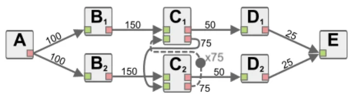
An example of an SDF graph with 5 actors is given in Figure 2. FIFOs are labeled with their token produc-tion and consumpproduc-tion rates. A FIFO with a dot signifies that initial tokens are present in the FIFO queue when the system starts to execute. The number of initial to-kens is specified by the xN label. Initial toto-kens are a semantic element of the SDF MoC that makes commu-nication possible between successive iterations of the graph execution; they are often used to pipeline the ex-ecution of applications described with SDF graphs [18]. Actors have no states in the SDF MoC, consequently if enough data tokens are available, an actor can start several executions in parallel. For example in Figure 2, actor A produces enough data tokens for actor B to be executed twice in parallel. Hence, the SDF MoC naturally expresses the parallelism of an application. However, because of its self-loop FIFO, the two firings of actor C cannot be executed simultaneously since the second firing requires data tokens produced by the first. Assigning a static order to the firings of the actors on the cores of a target architecture is called scheduling the application. 50 50 150 100 25 75 50 150 200

A

B

C

D

E

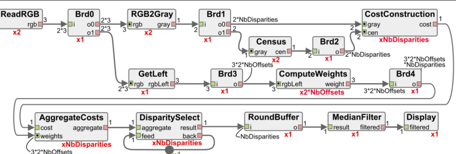
Our SDF graph of the stereo matching algorithm is presented in Figure 3. For the sake of readability, all the token production and consumption rates displayed in the SDF graph are simplified and should be multiplied by the number of input image pixels to obtain the real exchange rates. Below each actor, in bold, is a repetition factor which indicates the number of executions of this

actor during each iteration of the graph. This number of executions is deduced from the data productions and consumptions of actors. Two parameters are used in the graph: NbDisparities which represents the number of distinct values that can be found in the output disparity map, and NbOffsets which is a parameter influencing the size of the pixel area considered for the correlation calculus of the algorithm [37]. The SDF graph contains 12 distinct actors:

– ReadRGB produces the 3 color components of an input image by reading a stream or a file. This actor is called twice: once for each image of the stereo pair. – BrdX is a broadcast actor. Its only purpose is to duplicate on its output ports the data token con-sumed on its input port.

– GetLeft gets the RGB left view of the stereo pair. – RGB2Gray converts an RGB image into its

gray-scale equivalent.

– Census produces an 8-bit signature for each pixel of an input image. This signature is obtained by comparing each pixel to its 8 neighbors: if the value of the neighbor is greater than the value of the pixel, one signature bit is set to 1; otherwise, it is set to 0. – CostConstruction is executed once per possible disparity level. By combining the two images and their census signatures, it produces a value for each pixel that corresponds to the cost of matching this pixel from the first image with the corresponding pixel in the second image shifted by a disparity level. – ComputeWeights produces 3 weights for each pixel, using characteristics of neighboring pixels. ComputeWeights is executed twice for each offset: once considering a vertical neighborhood of pixels, and once with a horizontal neighborhood.

– AggregateCosts computes the matching cost of each pixel for a given disparity. Computations are based on an iterative method that is executed NbOffsets times.

– DisparitySelect produces a disparity map by com-puting the disparity of the input cost map from the lowest matching cost for each pixel. The first input cost map is provided by an AggregateCosts actor and the second input cost map is the result of a previous comparison.

– RoundBuffer forwards the last disparity map con-sumed on its input port to its output port.

– MedianFilter applies a 3×3 pixels median filter to the input disparity map to smooth the results. – Display displays the result of the algorithm or

writes it in a file.

This SDF description of the algorithm provides a high degree of parallelism since it is possible to execute in

4 Karol Desnos et al. ReadRGB 3 3 3 2*3 2*3 2 2 1 1 2 1 2*3 2*3 3 rgb 3*2*NbOffsets 3*2*NbOffsets 3*2*NbOffsets *NbDisparities 3 3 3*2*NbOffsets x1 NbDisparities 1 1 1 1 1 1 1 1 1 1 2*NbDisparities 2 2 2*NbDisparities Brd0 i o0 o1 rgb RGB2Gray gray GetLeft rgb rgbLeft cen cost Brd1 i o0 o1 Census gray cen Brd2 i o Brd3 i o weight Brd4 i o cost weights aggregate aggregate feed result back

i o result filtered filtered

gray CostConstruction DisparitySelect AggregateCosts rgbLeft Display MedianFilter RoundBuffer ComputeWeights x1 x2 x1 x1 x1 x2*NbOffsets x1 xNbDisparities xNbDisparities x1 x1 xNbDisparities x1 x2 x1 x2

Fig. 3 Stereo-matching SDF graph. All rates are implicitly multiplied by the picture size.

parallel the repetitions of the three most computation-ally intensive actors, namely CostConstruction, Aggre-gateCosts, and ComputeWeights. A detailed descrip-tion of the original stereo matching algorithm can be found in [37] and our open-source SDF implementation is available online [8].

2.3 Target architectures

In this paper, we consider the implementation of the stereo matching algorithm on two multicore architec-tures:

The i7-3610QM is a multicore Central Processing Unit (CPU) manufactured by Intel [15]. This 64bit pro-cessor contains 4 physical hyper-threaded cores that are seen as 8 virtual cores from the application side. This CPU has a clock speed of between 2.3GHz and 3.3GHz. Using virtual memory management technique, this CPU provides virtually unlimited memory resour-ces to the applications it executes.

The TMS320C6678 is multicore Digital Signal Pro-cessor (DSP) manufactured by Texas Instruments [32]. This MPSoC contains 8 C66x DSPs, each running at 1.0GHz on our experimental evaluation module. Although the size of the addressable memory spa-ce is 8Gbytes, the evaluation module contains only 512Mbytes of shared memory.

Contrary to the Intel’s CPU, the TMS320C6678 does not have a hardware cache coherence mechanism to manage the private caches of each of its 8 cores. Consequently, it is the developer’s responsibility to use writeback and invalidate functions to make sure that data stored in the two levels of private cache of each core is coherent.

The diverse memory characteristics and constraints of the two architectures must be taken into account

when implementing an application. Section 3 presents the memory challenges encountered when implementing the stereo matching application on these two architec-tures.

3 Challenges and Related Works

This section presents the 3 main challenges addressed in the paper and their related work.

3.1 Memory reuse

To our knowledge, minimizing the memory footprint of dataflow applications is usually achieved by using FIFO dimensioning techniques [24, 29, 22, 2]. FIFO dimension-ing techniques consist of finddimension-ing a schedule of the ap-plication that minimizes the memory space allocated to each FIFO of the SDF graph. For example, considering actors B and C from the graph of Figure 2, if the two repetitions of B are scheduled before the two repeti-tions of C (BBCC ), then the FIFO between the two actors must be allocated enough memory to store 300 data tokens. However, if the 2 executions of B and C are interleaved (BCBC ) then only 150 data tokens need to be stored in the FIFO. This technique is used in the most popular dataflow frameworks such as SDF3 [29], Ptolemy II [24], or Kalray’s dataflow tool chain [3].

The main drawback of FIFO dimensioning techni-ques is that they do not consider the reuse of memory since each FIFOs is allocated in a dedicated memory space. For example, if FIFO dimensioning is applied to the example of Figure 2, even though FIFOs AB and DE are never full simultaneously, they will not be allocated in overlapping memory spaces. Hence, FIFO dimensioning often results in wasted memory space [21].

As presented in Sections 4 to 6, memory reuse is a key aspect of the memory analysis and optimiza-tion techniques presented in this paper. Moreover, con-trary to most memory optimization techniques for SDF graphs that consider only monocore architectures [21, 29, 22], our method focuses on shared memory multicore processors.

3.2 Broadcast memory waste

An important challenge when implementing the stereo matching application is the explosion of the memory space requirements caused by the broadcast actors. For example in Figure 3, with NbOffsets = 5, NbDispari -ties = 60 and a resolution of 450*375 pixels, the broadcast actor Brd4 produces 3 ∗ 2 ∗ NbOffsets ∗ NbDispari -ties ∗ resolution float values, or 1.13Gbytes of data. Be-side the fact that this footprint alone largely exceeds the 512Mbytes capacity of the multicore DSP, this amount of memory is a waste as it consists only of 60 duplica-tions of the 19.3Mbytes of data produced by the firings of the ComputeWeights actor.

Non-destructive reads, or FIFO peeking, is a well-known way to read data tokens without consuming them, hence avoiding the need for broadcast actors [13]. Unfortunately, this technique cannot be applied with-out considerably modifying the underlying SDF MoC. Indeed, in the stereo matching example, using FIFO peeking would mean that the AggregateCosts only per-forms peeks and never consumes data tokens on its weights input port. Consequently, tokens would accu-mulate indefinitely on the FIFO connected to this port. In Section 6, we propose a non-invasive addition to the SDF MoC to solve the broadcast issue.

3.3 Cache coherence

Cache management is a key challenge when implement-ing an application on a multicore target without auto-matic cache coherence. Indeed, as shown in [33], the use of cache dramatically improves the performance of an application on multi-DSP architectures, with execution times up to 24 times shorter that without cache.

An automatic method to insert calls to writeback and invalidate functions in code generated from a SDF graph is presented in [33]. As depicted in Figure 4, this method is applicable for shared memory communica-tions between two processing elements. Actors A and B both have access to the shared memory addresses where data tokens of the AB FIFO are stored. The synchro-nization between cores is ensured by the Send and Recv actors which can be seen as post and pend semaphore

Core2 Shared memory Core2 cache Core1 cache Core1 Recv B Invalidate Writeback

Valid A-B data

Possibly invalid

A-B data

A Send

Fig. 4 Cache coherence solution without memory reuse

operations respectively. A writeback call is inserted be-fore the Send operation to make sure that all AB data tokens from Core1cache are written back in the shared memory. Similarly, an invalidate call is inserted after the Recv operation to make sure that cache lines corre-sponding to the address range of buffer AB are removed from Core2 cache.

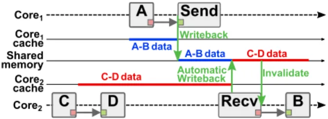
Core2 Shared memory Core2 cache Core1 cache Core1

Recv

D

B

C

A

Send

Fig. 5 Cache coherence issue with memory reuse

As depicted in Figure 5, a problem arises if the method presented in [33] is used jointly with memory reuse techniques. In this example, overlapping mem-ory spaces are used to store data tokens of two FIFOs: AB and CD. After the firings of actors C and D, the cache memory of Core2 is “dirty”, containing data to-kens of the CD FIFO that were not written back in the shared memory. Because these data tokens are “dirty”, the local cache manager might generate an automatic writeback to put new data in the cache. If however, as in the example, this automatic writeback occurs after the writeback from Core1, then the CD data tokens will overwrite AB tokens in the shared memory, thus cor-rupting the data accessed by actor B.

In addition to the memory reuse techniques pre-sented in Sections 4 and 5, we propose a solution to generate code for cache-incoherent multicore architec-ture in Section 6.

4 Memory Bounds

Bounding the amount of memory needed to implement an application on a targeted multicore architecture is a key step of a development process. Indeed, memory upper and lower memory bounds are crucial pieces of

6 Karol Desnos et al.

information in the co-design process, as they allow the developer to adjust the size of the architecture mem-ory according to the application requirements. Further-more, as these bounds can be computed during the early development of an MPSoC, they might assist the de-veloper in correct memory dimensioning (i.e. to avoid mapping an insufficient or an unnecessarily large mem-ory chip).

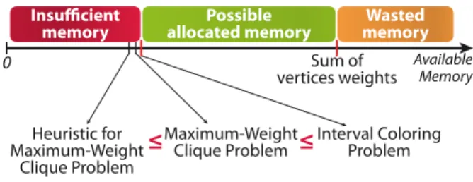
The technique presented in this section is an analy-sis technique for deriving the memory allocation bounds (Figure 6) of an application modeled with an SDF graph.

Insufficient

memory allocated memoryPossible memoryWasted

Available Memory Lower

Bound≤AllocationOptimal BoundUpper=AllocationWorst

0

Fig. 6 Memory Bounds

This bounding technique is applicable in every sta-ges of the development of an application, even when there is a complete abstraction of the system architec-ture. The bounding technique can be used both to pre-dict memory requirements of an application in the early stages of its development, and to assess the quality of an allocation result during the implementation of an ap-plication. This bounding technique was first introduced in [6]. It is presented in this paper as a necessary first step to our memory reuse techniques as well as a way to assess the quality of our allocation results in Section 7.

4.1 SDF graph pre-processing

The first step to derive the memory bounds of an ap-plication consists of successively transforming its SDF graph into a single-rate SDF and into a Directed Acyclic Graph (DAG) so as to reveal its embedded parallelism and model its memory characteristics.

As exposed in [3], the transformation of an SDF graph into its equivalent single-rate SDF can be ex-ponential in terms of number of actors. As a conse-quence, the method we propose should only be ap-plied to SDF graphs with a relatively coarse grained description: graphs whose single-rate equivalent have at most hundreds of actors and thousands of single-rate buffers [6]. Despite this limitation, the single-single-rate transformation has proven to be efficient for many real applications, notably in the telecommunication [25] and the multimedia [7] domains.

4.1.1 Pre-processing objectives

In the context of memory analysis and allocation, the single-rate and the DAG transformations are applied with the following objectives:

− Expose data parallelism: Concurrent analysis of data parallelism and data precedence gives information on the lifetime of memory objects prior to any sche-duling process. Indeed, two FIFOs belonging to paral-lel data-paths may contain data tokens simultaneously and are consequently forbidden from sharing a memory space. Conversely, two single-rate FIFOs linked with a precedence constraint can be allocated in the same memory space since they will never store data tokens simultaneously. In Figure 7 for example, FIFO AB1 is a predecessor to C1D1. Consequently, these two FIFOs may share a common address range in memory.

− Break FIFOs into shared buffers: The memory needed to allocate each FIFO corresponds to the maxi-mum number of tokens stored in the FIFO during an iteration of the graph [21]. However, in our method, the memory allocation can be independent from scheduling considerations. It is for this reason that FIFOs of unde-fined size before the scheduling step are replaced with buffers of fixed size during the transformation of the graph into a single-rate SDF.

− Derive an acyclic model: In the absence of a schedule, deriving a DAG permits the use of single-rate FIFOs that will be written and read only once per it-eration of this DAG. Consequently, before a single rate FIFO is written and after it is read, its memory space will be reusable to store other objects.

4.1.2 Graph transformations

The first transformation applied to the input SDF graph to reveal parallelism is a conversion into a single-rate SDF graph. A single-single-rate SDF graph is an SDF graph where the production and consumption rates on each FIFO are equal. Each vertex of the single-rate SDF graph corresponds to a single actor firing from the SDF graph. This conversion is performed by com-puting the topology matrix [18], by duplicating actors by their number of firings, and by connecting FIFOs properly. For example, in Figure 7, actors B, C, and D are each split in two instances and new FIFOs are added to ensure the equivalence with the SDF graph of Figure 2. An algorithm to perform this conversion can be found in [28].

The second conversion consists of generating a Di-rected Acyclic Graph (DAG) by isolating one itera-tion of the algorithm. This conversion is achieved by ignoring FIFOs with initial tokens in the single-rate

75 75 50 50 150 150

A

C

C

E

D

D

B

B

Fig. 7 Single-rate SDF graph. (Directed Acyclic Graph (DAG) if dotpoint FIFO is ignored)

SDF graph. In our example, this approach means that the feedback FIFO C2C1, which stores 75 initial to-kens, is ignored. Our optimization technique does not allow the concurrent execution of successive iterations of the graph since the lifetime of each memory object is bounded by the span of a graph iteration. As presented in [18], delays can be added to acyclic data-paths of a dataflow graph in order to pipeline an application. By doing so, the developer can divide a graph into several unconnected graphs whose iterations can be executed in parallel, thus improving the application throughput. From the memory perspective, pipelining a graph will increase the graph parallelism and consequently the amount of memory required for its allocation. In the case of stereo matching, the addition of a pipeline stage after the AggregateCost actor leads to an increase of the memory footprint by 50%. However, since the critical path is largely dominated by the most parallel actors, pipelining this application does not lead to a substan-tial throughput improvement.

4.1.3 Memory objects

The DAG resulting from the transformations of an SDF graph contains three types of memory objects:

− Communication buffers: The first type of mem-ory object, which corresponds to the single-rate FIFOs of the DAG, are the buffers used to transfer data to-kens between consecutive actors. In our approach, we consider that the memory allocated to these buffers is reserved from the execution start of the producer actor until the completion of the consumer actor. This choice is made to enable custom token accesses throughout ac-tor firing time. As a consequence, the memory used to store an input buffer of an actor should not be reused to store an output buffer of the same actor. In Figure 7, the memory used to carry the 100 data tokens between actors A and B1 can not be reused, even partially, to transfer data from B1 to C1.

− Working memory of actors: The second type of memory object corresponds to the maximum amount of memory allocated by an actor during its execution. This working memory represents the memory needed to store the data used during the computations of the ac-tor but does not include the input buffer nor the output

buffer storage. In our method, we assume that an actor keeps exclusive access to its working memory during its execution. This memory is equivalent to a task stack space in an operating system.

− Feedback/Pipeline FIFOs: The last type of mem-ory object corresponds to the memmem-ory needed to store feedback FIFOs ignored by the transformation of a single-rate SDF into a DAG. In Figure 7, there is a single feedback FIFO between C2 and C1. Each feed-back FIFO is composed of 2 memory objects: the head and the (optional) body. The head of the feedback FIFO corresponds to the data tokens consumed during an it-eration of the single-rate SDF. A head memory object may share memory space with any buffer that is both a successor to the actor consuming tokens from the feed-back FIFO and a predecessor to the actor producing tokens on the feedback FIFO.

The body of the feedback FIFO corresponds to data tokens that remain in the feedback FIFO for several iterations of the graph before being consumed. A body memory object is needed only if the amount of delay on the feedback FIFO is greater than its consumption rate. A Body memory object must always be allocated in a dedicated memory space.

4.2 Memory Exclusion Graph (MEG)

Once an application SDF graph has been transformed into a DAG and all its memory objects have been iden-tified, we derive a Memory Exclusion Graph (MEG) which will serve as a basis to our analysis and alloca-tion techniques.

A Memory Exclusion Graph (MEG) is an undirec-ted weighundirec-ted graph denoundirec-ted by G =< V, E, w > where: – V is the set of vertices. Each vertex represents an

indivisible memory object.

– E is the set of edges representing the memory ex-clusions, i.e. the impossibility to share memory. – w : V → N is a function with w(v) the weight of a

vertex v. The weight of a vertex corresponds to the size of the associated memory object.

– N(v) the neighborhood of v, i.e. the set of vertices linked to v by an exclusion e ∈ E. Vertices of this set are said to be adjacent to v.

– |S| the cardinality of a set S. |V | and |E| are the number of vertices and edges respectively of a graph. – δ(G) = _{|V |·(|V |−1)}2·|E| the edge density of the graph corresponding to the ratio of existing exclusions to all possible exclusions.

Two memory objects of any type exclude each other (i.e. they can not be allocated in overlapping address

8 Karol Desnos et al.

ranges) if the DAG can be scheduled in such a way that both these memory objects store data simultaneously. Some exclusions are directly caused by the properties of the memory objects, such as exclusions between in-put and outin-put buffers of an actor. Other exclusions result from the parallelism of an application, as is the case with the working memory of actors that might be executed concurrently because they belong to parallel data-paths. C1C2 75 D1E 25 D2E 25 C2D2 50 C1D1 50 B2C2 150 B1C1 150 AB₁₀₀2 AB1 100

A

E

B

B

C

C

D

D

CPU1 schedule _CPU2 schedule

A

B

C

D

E

A

D

E

B

C

h

E

D

Fig. 8 Memory Exclusion Graph (MEG) derived from Fig. 2

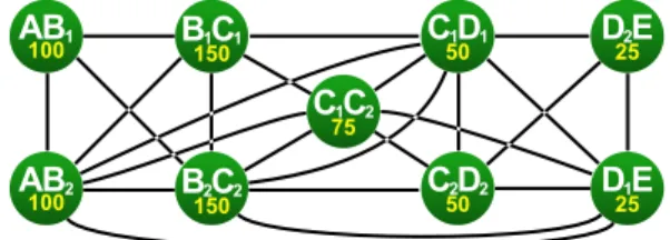
The MEG presented in Figure 8 is derived from the SDF graph of Figure 2. The complete MEG contains 18 memory objects and 69 exclusions but, for clarity, only the vertices corresponding to the buffers between actors (1st _{type memory objects) are presented. The} values printed below the vertices names represent the weight w of the memory objects.

The pseudo-code of an algorithm to build the com-plete MEG of an application is given in Figure 9.

The MEG obtained at this point of the method is a worst-case scenario since it models all possible ex-clusions for all possible schedules. As will be shown in Section 5, it is possible to update a MEG with sche-duling information in order to reduce the number of exclusion, thus favoring memory reuse.

4.3 Bounding techniques

The upper and lower bounds of the static memory allo-cation of an appliallo-cation are a maximum and a minimum limit respectively to the amount of memory needed to run an application, as presented in Figure 6. The fol-lowing four sections explain how the upper bound can be computed and give three techniques to compute the memory allocation lower bound. These three techniques offer a trade-off between accuracy of the result (Fig-ure 10) and complexity of the computation.

4.3.1 Least upper bound

The least upper memory allocation bound of an appli-cation corresponds to the size of the memory needed

Input: a single-rate SDF srSDF =< A, F > with: A the set of actors

F the set of FIFOs

Output: a Memory Exclusion Graph M EG =< V, E, w > 1: Define P red[], I[], O[] : A → V∗_{⊂ V}

2: Sort A in the DAG precedence order 3: for each a ∈ A do

4: /* Process working memory of a */ 5: workingM em ← new v ∈ V

6: w(workingM em) ← workingM emorySize(a) 7: for each v ∈ V \ {P red[a], workingM em} do 8: Add e ∈ E between workingM em and v 9: end for

10: I[a] ← I[a] ∪ {workingM em} 11: /* Process output buffers of a */

12: for each f ∈ (F \ f eedbackF IF Os) ∩ outputs(a) do 13: buf M em ← new v ∈ V

14: w(buf M em) ← size(f )

15: for each v ∈ V \ {P red[a], buf M em} do 16: Add e ∈ E between buf M em and v 17: end for

18: P red[consumer(f )] ← P red[a] ∪ I[a]

19: I[consumer(f )] ← I[consumer(f )] ∪ {buf M em} 20: O[a] ← O[a] ∪ {buf M em}

21: end for 22: end for

23: /* Process Feedback FIFOs */

24: for each ff ∈ F ∩ f eedbackF IF Os(F ) do 25: headM em ← new v ∈ V

26: w(headM em) ← rate(ff )

27: set ← (V ∩ P [producer(ff )]) \ P [consumer(ff )] 28: set ← set \ I[consumer(ff )] ∪ O[consumer(ff )] 29: for each v ∈ V \ set do

30: Add e ∈ E between headM em and v 31: end for

32: if rate(ff ) < delays(ff ) then 33: bodyM em ← new v ∈ V

34: w(bodyM em) ← delays(ff ) − rate(ff ) 35: for each v inV do

36: Add e ∈ E between bodyM em and v 37: end for

38: end if 39: end for

Fig. 9 Building the Memory Exclusion Graph (MEG)

to allocate each memory object in a dedicated memory space. This allocation scheme is the least compact al-location possible as a memory space used to store an object would never be reused to store another.

Given a MEG G, its upper memory allocation bound is thus the sum of the weight of its vertices:

BoundM ax(G) = X

v∈V

w(v) (1)

The upper bound for the MEG of Figure 8 is 725 units. As presented in Figure 10, using more memory than the upper bound means that part of the memory re-sources is wasted. Indeed, if a memory allocation uses an address range larger than this upper bound, some addresses within this range will never be read nor writ-ten.

Memory Analysis and Optimized Allocation of Dataflow Applications on Shared-Memory MPSoCs 9

Insufficient

memory allocated memoryPossible memoryWasted

Available Memory Maximum-Weight Clique Problem Heuristic for Maximum-Weight Clique Problem

≤

≤

memory allocated memory memory

Available Memory Lower Bound₌ Optimal Allocation Upper Bound₌ Worst Allocation 0

Fig. 10 Computing the lower memory bound

4.3.2 Method 1 to compute the greatest lower bound -Interval Coloring Problem

The greatest lower memory allocation bound of an ap-plication is the least amount of memory required to execute it. Finding this optimal allocation based on a MEG can be achieved by solving the equivalent Interval Coloring Problem [4, 12].

A k-coloring of a MEG is the association of each vertex vi of the graph with an interval Ii = {a, a + 1, · · · , b−1} of consecutive integers - called colors -, such that b−a = w(v). Two distinct vertices viand vjlinked by an edge must be associated to non-overlapping in-tervals. Assigning an interval to a weighted vertex is equivalent to allocating a range of memory addresses to a memory object. Consequently, a k-coloring of a MEG corresponds to an allocation of its memory objects.

The Interval Coloring Problem consists of finding a k-coloring of the exclusion graph with the fewest inte-gers used in the Ii intervals. This objective is equiv-alent to finding the allocation of memory objects that uses the least memory possible, thus giving the greatest lower bound of the memory allocation.

Unfortunately, as presented in [4], this problem is known to be NP-Hard, therefore it would be prohibi-tively long to solve for applications with hundreds or thousands of memory objects. Moreover, a sub-optimal solution to the Interval Coloring problem corresponds to an allocation that uses more memory than the mini-mum possible: more memory than the greatest lower bound. Consequently, a sub-optimal solution fails to achieve our objective which is to find a lower bound to the size of the memory allocated for a given applica-tion.

4.3.3 Method 2 to compute a lower bound - Exact solution to the Maximum-Weight Clique Problem Since the greatest lower bound can not be found in reasonable time, we focus our attention on finding a lower bound close to the size of the optimal allocation. In [12], Fabri introduces another lower bound derived

from an exclusion graph: the weight of the Maximum-Weight Clique (MWC).

A clique is a subset of vertices that forms a sub-graph within which each pair of vertices is linked with an edge. As memory objects of a clique can not share memory space, their allocation requires a memory as large as the sum of the weights of the clique elements, also called the clique weight. Subsets S1:={AB1, AB2, B2C2} and S2:={C1D1, D2E, C2D2, D1E} are exam-ples of cliques in the MEG of Figure 8. Their respective weights are 350 and 150. By definition, a single ver-tex can also be considered as a clique. A clique is called maximal if no vertex can be added to it to form a larger clique. In Figure 8, clique S2 is maximal, but clique S1 is not as B1C1 is linked to all the clique vertices and can therefore be added to the clique.

The Maximum-Weight Clique (MWC) of a graph is the clique whose weight is the largest of all cliques in the graph. Although this problem is also known to be NP-Hard, several algorithms have been proposed to solve it efficiently. In [23], ¨Osterg˚ard proposes an exact algo-rithm which is, to our knowledge, the fastest algoalgo-rithm for MEGs with an edge density under 0.80. For graphs with an edge density above 0.80, a more efficient algo-rithm was proposed by Yamaguchi et al in [36]. Both algorithms are recursive and use a similar branch-and-bound approach. Beginning with a subgraph composed of a single vertex, they search for the MWC Ci in this subgraph. Then, a vertex is added to the considered subgraph, and the weight of Ci is used to bound the search for a larger clique Ci+1 in the new subgraph. In [6], the two algorithms were implemented to compare their performances on exclusion graphs derived from different applications. In the exclusion graph of Fig-ure 8, the MWC is {AB2,B1C1,B2C2,C1C2,C1D1} with a weight of 525 units.

The weight of the MWC corresponds to the amount of memory needed to allocate the memory objects be-longing to this subset of the graph. By extension, the allocation of the whole graph will never use less mem-ory than the weight of its MWC. Therefore, this weight is a lower bound to the memory allocation and is less than or equal to the greatest lower bound, as shown in Figure 10.

4.3.4 Method 3 to compute a lower bound - Heuristic for the Maximum-Weight Clique Problem

¨

Osterg˚ard’s and Yamaguchi’s algorithms are exact al-gorithms and not heuristics. Since the MWC problem is an NP-Hard problem, finding an exact solution in polynomial time can not be guaranteed. For this

rea-10 Karol Desnos et al.

son, we have developed a heuristic algorithm for the MWC problem.

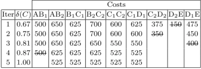
The proposed heuristic approach, presented in Fig-ure 11, is an iterative algorithm whose basic principle is to remove a judiciously selected vertex at each itera-tion, until the remaining vertices form a clique.

Input: a Memory Exclusion Graph G =< V, E, w > Output: a maximal clique C

1: C ← V 2: nbedges← |E| 3: for each v ∈ C do 4: cost(v) ← w(v) +P v0_{∈N (v)}w(v0) 5: end for

6: while |C| > 1 and 2·nbedges

|C|·(|C|−1)< 1.0 do

7: Select v∗from V that minimizes cost(·) 8: C ← C \ {v∗_} 9: nbedges← nbedges− |N (v∗) ∩ C| 10: for each v ∈ N (v∗_{) ∩ C do} 11: cost(v) ← cost(v) − w(v∗₎ 12: end for 13: end while

14: Select a vertex vrandom∈ C

15: for each v ∈ N (vrandom) \ C do

16: if C ⊂ N (v) then 17: C ← C ∪ {v} 18: end if

19: end for

Fig. 11 Maximum-Weight Clique Heuristic Algorithm

Our algorithm can be divided into 3 parts:

– Initializations (lines 1-5): For each vertex of the MEG, the cost function is initialized with the weight of the vertex summed with the weights of its neigh-bors. In order to keep the input MEG unaltered through the algorithm execution, its set of vertices V and its number of edges |E| are copied in local variables C and nbedges.

– Algorithm core loop (lines 6-13): During each it-eration of this loop, the vertex with the minimum cost v∗ is removed from C (line 8). In the few cases where several vertices have the same cost, the low-est number of neighbor |N (v)| is used to determine the vertex to remove. If the number of neighbors is equal, then selection is performed based on the smallest weight w(v). By doing so, the number of edges removed from the graph is minimized and the edge density of the remaining vertices will be higher, which is desirable when looking for a clique. If there still are multiple vertices with equal properties, a random vertex is selected among them.

This loop is iterated until the vertices in subset C become a clique. This condition is checked line 6, by comparing 1.0 (the edge density of a clique) with the edge density of the subgraph of G formed by the remaining vertices in C. To this purpose nbedge, the

number of edges of this subgraph, is decremented line 9 by the number of edges in E linking the re-moved vertex v∗to vertices in C. Lines 10 to 12, the costs of the remaining vertices are updated for the next iteration.

– Clique maximization (lines 14-19): This last part of the algorithm ensures that the clique C is maximal by adding neighbor vertices to it. To become a mem-ber of the clique, a vertex must be adjacent to all its members. Consequently, the candidates to join the clique are the neighbors of a vertex randomly selected in C. If a vertex among these candidates is linked to all vertices in C, it is added to the clique. The complexity of this heuristic algorithm is of the or-der of O(|N |2_{), where |N | is the number of vertices of} the MEG.

In Table 1, the algorithm is applied to the MEG of Figure 8. For each iteration, the costs of the remaining vertices are given, and the vertex removed during the iteration is crossed out. The column δ(C) corresponds to the edge density of the subgraph formed by the re-maining vertices. For example, in the first iteration, the memory object D2E has the lowest cost and is thus re-moved from the MEG. Before beginning the second it-eration, the costs of memory objects C1D1, C2D2, and D1E are decremented by 25: the weight of the removed memory object. Costs Iter δ(C) AB1AB2B1C1B2C2C1C2C1D1C2D2D2E D1E 1 0.67 500 650 625 700 600 625 375 150 475 2 0.75 500 650 625 700 600 600 350 450 3 0.81 500 650 625 650 550 550 400 4 0.87 500 625 625 625 525 525 5 1.00 525 525 525 525 525

Table 1 Algorithm proceeding for the MEG of Figure 8

In this simple example, the clique found by the heu-ristic algorithm and the exact algorithm are the same, and their weight also corresponds to the size of the op-timal allocation. This example proves that, as shown in Figure 10, the result of the heuristic can be equal to the exact solution of the MWC problem, whose size can also equal that of the optimal allocation.

5 Memory Allocation Strategies

Given an initial MEG constructed from a non-scheduled DAG, we propose three possible implementation stages to perform the allocation of this MEG in shared mem-ory: prior to any scheduling process, after an untimed

Memory Analysis and Optimized Allocation of Dataflow Applications on Shared-Memory MPSoCs 11

multicore scheduling of actors, or after a timed multi-core scheduling of the application. The scheduling flex-ibility resulting from the three alternatives are detailed in the following subsections.

5.1 Memory Exclusion Graph (MEG) updates

As presented in Section 4.2, the MEG built from the non-scheduled DAG is a worst-case scenario as it mod-els all possible exclusions for all possible schedules of the application on any number of cores. If a multicore schedule of the application is known, this schedule can be used to update the MEG and lower its density of exclusions.

Scheduling a DAG on a multicore architecture intro-duces an order of execution of the graph actors, which is equivalent to adding new precedence relationships be-tween actors. Adding new precedence edges to a DAG results in a decreased inherent parallelism of the ap-plication. For example, Figure 12 illustrates the new precedence edges that result from scheduling the DAG on 2 cores. In this example, Core1 executes actors B1, C1, D1 and D2; and Core2 executes actors A, B2, C2 and E . 75 75 50 50 150 150

A

C

C

E

D

D

B

B

Core1 Schedule Core2 Schedule

Fig. 12 Scheduled Single-rate SDF graph

As presented in Section 4.2, memory objects belong-ing to parallel data-paths may have overlappbelong-ing life-times. Reducing the parallelism of an application re-sults in creating new precedence paths between memory objects, thus preventing them from having overlapping lifetimes and removing exclusions between them. Since all the parallelism embedded in a DAG is explicit, the scheduling process cannot augment the parallelism of an application and cannot create new exclusions be-tween memory objects. Figure 13 illustrates the up-dated MEG resulting from the multicore schedule of Figure 12.

A second update of the MEG is possible if a timed schedule of the application is available. A timed sched-ule is a schedsched-ule where not only the execution order of the actors is fixed, but also their absolute starting and ending times. Such a schedule can be derived if the exact, or the worst-case execution times of all actors

C1C2 75 D1E 25 D2E 25 C2D2 50 C1D1 50 B2C2 150 B1C1 150 AB₁₀₀2 AB1 100

A

B

E

B

C

C

D

D

Core1 schedule Core2 schedule

A

B

C

D

E

A

D

E

B

C

h

E

D

Fig. 13 MEG updated with schedule from Figure 12

are known at compile time [25]. Updating a DAG with a timed schedule consists of adding precedence edges between all actors with non-overlapping lifetimes.

Following assumptions made in Section 4.1, the life-time of a memory object begins with the execution start of its producer, and ends with the execution end of its consumer. In the case of working memory, the lifetime of the memory object is equal to the lifetime of its as-sociated actor. Using a timed schedule, it is thus pos-sible to update a MEG so that exclusions remain only between memory objects whose lifetimes overlap. For example, the timed schedule of Figure 14(a) introduces a precedence relationship between actors B2 and C1 which translates into removing the exclusion between AB2and C1D1 from the MEG.

5.2 Static MEG allocation

Allocating a MEG in memory consists of statically as-signing an address range to each memory object. Possi-ble approaches to perform the memory allocation are:

– Running an online allocation (greedy) algorithm. Online allocators assign memory objects one by one in the order in which they are fed to the allocator. Performance of online algorithms can be greatly im-proved by feeding the allocator with memory objects sorted in a smart order [7]. The most commonly used online allocators are the First-Fit (FF) and the Best-Fit (BF) algorithms [16]. FF algorithm consists of allocating an object to the first available space in memory of sufficient size. The BF algorithm works similarly but allocates each object to the available space in memory whose size is the closest to that of the allocated object.

– Running an offline allocation algorithm [14, 21]. In contrast to online allocators, offline allocators have a global knowledge of all memory objects requiring allocation, thus making further optimizations possi-ble.

– Coloring the MEG. Each vertex of the graph is asso-ciated with a set of colors such that two connected vertices have no color in common. The purpose of

12 Karol Desnos et al.

graph coloring technique is to minimize the total number of colors used in the graph [4].

– Using constraint programming [31] where memory constraints can be specified together with resource usage and execution time constraints.

In addition to these static allocation techniques, which are executed during the compilation of the application, dynamic allocation techniques can also be used. Dy-namic allocation consists of allocating the memory ob-jects of the MEG during the execution of the applica-tion. To keep the runtime overhead of dynamic allo-cation as low as possible, lightweight alloallo-cation algo-rithms such as the FF or the BF allocators are com-monly used [16, 32].

5.3 Pre-scheduling allocation

Before scheduling the application, the MEG models all possible exclusions that may prevent memory objects from being allocated in the same memory space. Hence, a pre-scheduling MEG models all possible exclusions for all possible multicore schedules of an application. Consequently, a compile-time allocation based on a pre-scheduling MEG will never violate any exclusion for any valid multicore schedule of this graph on any shared-memory architecture.

Since a compile-time memory allocation based on a pre-scheduling MEG is compatible with any multicore schedule, it is also compatible with any runtime sched-ule. The great flexibility of this first allocation approach is that it supports any runtime scheduling policy for the DAG and can accommodate any number of cores that can access a shared memory.

A typical scenario where this pre-scheduling compile-time allocation is useful is a multicore archi-tecture implementation which runs multiple applica-tions concurrently. In such a scenario, the number of cores used for an application may change at runtime to accommodate applications with high priority or those with high processing needs. The compile-time alloca-tion relieves runtime management from the weight of a dynamic allocator while guaranteeing a fixed memory footprint for the application.

The downside of this first approach is that, as will be shown in the results of Section 7, this allocation tech-nique requires substantially more memory than post-scheduling allocators.

5.4 Post-scheduling allocation

Post-scheduling memory allocation offers a trade-off be-tween amount of allocated memory and multicore

sche-duling flexibility. The advantage of post-schesche-duling over pre-scheduling allocation is that updating the MEG greatly decreases its density which results in using less allocated memory [7].

Like pre-scheduling memory allocation, the flexibil-ity of post-scheduling memory allocation comes from its compatibility with any schedule obtained by adding new precedence relationships to the scheduled DAG. Indeed, adding new precedence edges will make some exclusions useless but it will never create new exclu-sions. Any memory allocation based on the updated MEG of Figure 13 is compatible with a new schedule of the DAG that introduces new precedence edges. For example, we consider a single core schedule derived by combining schedules of Core1 and Core2 as follows A B2, B1, C1, C2, D1, D2 and E . Updating the MEG with this schedule would result in removing the exclu-sions between AB2 and {B1C1, C1C2, C1D1, D1E }.

The scheduling flexibility for post-scheduling alloca-tion is inferior to the flexibility offered by pre-schedu-ling allocation. Indeed, the number of cores allocated to an application may be only decreased at runtime for post-scheduling allocation while pre-scheduling alloca-tion allows the number of cores to be both increased and decreased at runtime.

5.5 Post-Timing allocation

A MEG updated with a timed schedule has the lowest density of the three alternatives, which leads to the best results in terms of allocated memory size. However, its reduced parallelism makes it the least flexible scenario in terms of multicore scheduling and runtime execution.

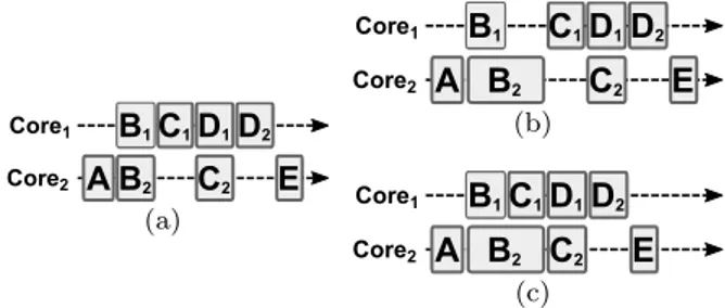
Core2 Core1 C1D1D2 C2 B1 B2 E A (a) Core2 Core1 B1 B2 D2 C1D1 C2 E A (b) Core2 Core1 C1D1D2 C2 B1 B2 E A (c)

Fig. 14 Loss of runtime flexibility with timed allocation. (a) Timed schedule for the graph of Figure 12.

(b)(c) Execution Gantt charts for timed and post-scheduling allocation with a doubled execution time for actor B2.

Figure 14 illustrates the possible loss of flexibility resulting from the usage of post-timing allocation. In the timed schedule of Figure 14(a), the same memory space can be used to store buffers AB2and C1D1since

Memory Analysis and Optimized Allocation of Dataflow Applications on Shared-Memory MPSoCs 13

B2 execution ends before C1 execution starts. In Fig-ures 14(c) and 14(b), we consider that the execution time of actor B2 is double that of the timed sched-ule. With timed allocation (Figure 14(b)), the execution of C1 must be delayed until B2 completion, or other-wise C1 might overwrite and corrupt data of the AB2 buffer. With post-scheduling allocation (Figure 14(c)), only the actor order on each core must be guaranteed. C1 can thus start its execution before B2 completion since buffers AB2 and C1D1 exclude each other in the corresponding MEG (Figure 13).

Although timed allocation provides the smallest mem-ory footprints [7], its lack of runtime flexibility makes it a bad option for implementation. Nevertheless, com-puting the memory bounds for a MEG updated with a timed schedule is a convenient way to approximate the memory footprint that would be allocated by a dynamic allocator. Using dynamic allocation consists of dynam-ically allocating each buffer when it is first needed and freeing it when it has been consumed. Static timed al-location and dynamic alal-location reach similar memory footprints as they both allow memory reuse as soon as the lifetime of a buffer is over.

A comparison of the three allocation strategies is available in [7] and their application to the stereo matching algorithm will be presented in Section 7.

6 Solutions to Implementation Issues 6.1 Zero-copy broadcasts

The memory waste produced by the broadcast actors of an SDF graph is illustrated in Figure 15. As intro-duced in Section 3.2, the only purpose of the broadcast actor of Figure 15(a) is to duplicate the n data tokens produced by actor A to provide a copy of these data to-kens to actors B, C, and D. In the corresponding MEG (Figure 15(b)), each FIFO connected to the broadcast actor is associated with a separate memory object of size n. Following the rules presented in Section 4.1, ex-clusions are added between all memory objects. Since the 4 memory objects form a clique, their allocation re-quires enough memory to store 4 ∗ n data tokens. Since all 4 memory objects store identical data, this pattern can be seen to be a waste of memory.

During its execution, an SDF actor can use its input buffers as scratchpad memory and write new values in these memory spaces. Duplicating the broadcasted data tokens is thus necessary to make sure that the data in the input buffer of an actor is not corrupted by the activity of another actor.

Our solution to avoid the waste of memory caused by broadcast actors is to allow the developer to specify

D

B

C

A

Brd

C

C

D

E

D

E

C

D

C

D

B

C

B

C

AB

AB

A

E

B

B

C

C

D

D

Core1 schedule Core2 schedule

A

B

C

D

E

A

D

E

B

C

h

E

D

whether an actor uses its input buffers as scratchpad memories or if it only reads the consumed values. In Figure 15(a) and Figure 3, read only input ports are marked with a black dot within the port anchor. Be-cause actors B and D have a read only input port, a private copy of the broadcasted data tokens is no longer needed and both actors can have a direct access to the ABrd memory object. Actor C however requires a private copy of the data tokens since it does not have a read only input port. Consequently, adding the read only information allows us to merge the memory objects ABrd, BrdB, and BrdD as a single memory object of size n. As a result, only 2 ∗ n memory units are needed to allocate the SDF graph of Figure 15(a), or half as much as the original memory requirement.

Contrary to FIFO peeking [13], our buffer merging technique does not require any change of the underly-ing SDF MoC. Similarly to annotations of imperative languages, marking an input port with the read only at-tribute does not have any effect on the behavior of the application. Indeed, read only attributes can be ignored during graph transformations and during the schedu-ling of the application and can be optionally used to reduce the memory footprint during the memory allo-cation process.

In addition to a drastic reduction of the memory footprint of the application, buffer merging also im-proves the performance of the application. Since the input buffers with a read only attribute are merged with the broadcasted buffer, the copy operation asso-ciated to these buffers is no longer needed. As shown in Section 7, these zero-copy broadcasts have a pos-itive impact on the application performance both on the multicore DSP and the CPU targets.

6.2 Automatic cache coherence

The cache coherence mechanism presented in Sec-tion 3.3 is incompatible with memory reuse techniques. As presented in Figure 5, the insertion of writeback and invalidate calls around inter-core synchronization ac-tors Send and Recv may result in data corruption in cases where a memory space is reused to store data

to-14 Karol Desnos et al.

kens from several buffers. This data corruption is caused by the automatic writeback of dirty lines of cache cor-responding to a reused memory space.

Core2 Shared memory Core2 cache Core1 cache Core1

Recv

D

B

C

A

Send

Fig. 16 Multicore cache coherence solution

Our solution to prevent unwanted writebacks is to make sure that no dirty lines of cache remain once the data tokens of a FIFO have been consumed. To this purpose, a call to the invalidate function is inserted for each buffer, after the firing of the actor consuming this buffer. As illustrated in Figure 16, the new calls to invalidate replace those inserted after the Recv syn-chronization actor.

As shown in Section 7, this solution allows us to ac-tivate the cache of the multicore DSP, leading to a huge improvement of the stereo-matching algorithm perfor-mance.

7 Experiments

7.1 Hardware/software exploration workflow

The stereo matching algorithm and the memory anal-ysis and optimization presented in this paper were im-plemented within a rapid prototyping framework called Preesm. Preesm (the Parallel and Real-time Embed-ded Executives Scheduling Method) is an open source framework developed at the IETR for research and ed-ucational purposes [25]. Rapid prototyping consists of extracting information from a system in the early stages of its development. It enables hardware/software co-design and favors early decisions that improve system architecture efficiency.

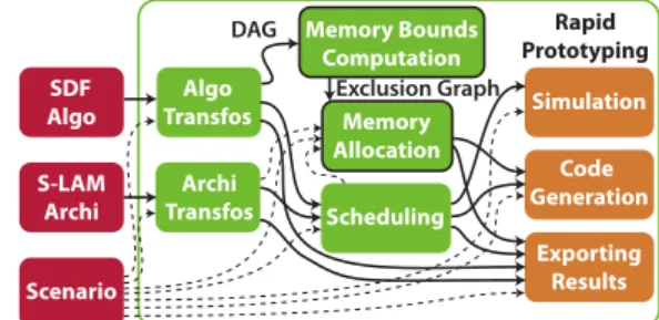
Figure 17 illustrates the position of the memory analysis and optimization techniques in the rapid pro-totyping process of Preesm [25]. Inputs of the rapid prototyping process consist of: an algorithm model re-specting the SDF MoC, an architecture model respect-ing the System-Level Architecture Model (S-LAM) se-mantics [26], and a scenario providing constraints and prototyping parameters. The scenario ensures the com-plete separation of algorithm and architecture models. In Preesm, algorithm and architecture models first undergo transformations in preparation for the rapid

Rapid Prototyping EESDF Algo S-LAM Archi Scenario Algo Transfos Archi Transfos Scheduling Simulation CodeE Generation Exporting Results MemoryEBounds Computation DAG Memory Allocation Exclusion Graph

Fig. 17 Preesm rapid prototyping process

prototyping steps. Then, static multicore scheduling is executed to dispatch and schedule the algorithm actors to the architecture processing elements [25, 5]. Finally, the multicore scheduling information is used to simulate the system behavior and to generate compilable code for the targeted architecture.

The complete independence between the architec-ture and algorithm models simplifies the porting of an application on different targets. For example, once the stereo-matching algorithm of Figure 3 was developed and tested on the Intel’s CPU, it took only two hours to adapt the readRGB and display actors and generate a functional version for the 8 cores of the C6678 mul-ticore DSP. Afterwards, it takes only a few seconds to generate code for one of the two multicore architectures. The Preesm project of the stereo matching appli-cation studied in this paper is available online [8].

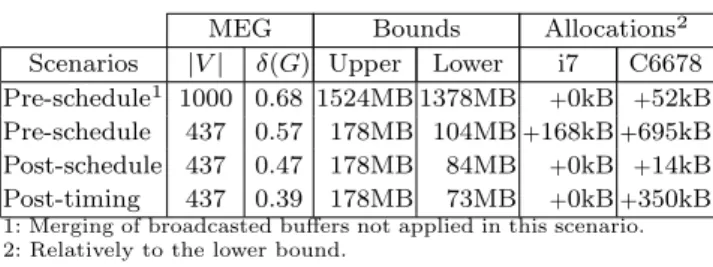
7.2 Memory study of the stereo matching algorithm Table 2 shows the memory characteristics resulting from the application of the techniques presented in this paper to the SDF graph of the stereo matching algo-rithm. The memory characteristics of the application are presented for 4 scenarios, each corresponding to a different implementation stage of the algorithm. The |V | and δ(G) columns respectively give the number of memory objects and the density of exclusion of the MEG. The next two columns present the upper and lower allocation bounds for each scenario. Finally, the last two columns present the actual amount of mem-ory allocated for each target architecture. The alloca-tion results are expressed as the supplementary amount of memory allocated compared to the lower bound. These results were obtained with NbOffsets = 5, Nb-Disparities = 60 and a resolution of 450*375 pixels. 7.2.1 Effect of broadcast merging

A comparison between the two pre-schedule scenarios of Table 2 reveals the impact of the merging of

broad-MEG Bounds Allocations2

Scenarios |V | δ(G) Upper Lower i7 C6678 Pre-schedule1 _{1000 0.68 1524MB 1378MB +0kB +52kB}

Pre-schedule 437 0.57 178MB 104MB+168kB+695kB Post-schedule 437 0.47 178MB 84MB +0kB +14kB Post-timing 437 0.39 178MB 73MB +0kB+350kB

1: Merging of broadcasted buffers not applied in this scenario. 2: Relatively to the lower bound.

Table 2 MEGs characteristics and allocation results

casted buffers presented in Section 6.1. The first pre-schedule scenario presented in the table corresponds to the memory characteristics of the stereo matching application when buffer merging is not applied. With a memory footprint of 1378Mbytes, this scenario for-bid the allocation of the application in the 512Mbytes shared memory of the multicore DSP. The application of the buffer merging technique in the second scenario leads to a reduction of the memory footprint by 92%, from 1378Mbytes to 104Mbytes.

Another positive aspect of the buffer merging tech-nique is the simplification of the MEG. Indeed, 563 ver-tices are removed from the MEG as a result of the buffer merging technique. The computation of the memory bounds of the MEG and the allocation of the MEG in memory are both accelerated by a factor of 6 with the simplified MEG.

In addition to the large reduction of the memory footprint, buffer merging also has a positive impact on the application performance. On the i7 multicore CPU, the stereo matching algorithm reaches a throughput of 1.84 frames per second (fps) when the broadcasted buffers are not merged, and a throughput of 3.50 fps otherwise. Hence, the suppression of the memcpy re-sults in a speedup ratio of 90%. On the C6678 DSP, the suppression of the memcpy results in a speedup ra-tio of 40%, rising from 0.24fps to 0.34fps.

7.2.2 Memory footprints

Results presented in Table 2 reveal the memory sav-ings resulting from the application of the memory reuse techniques presented in this paper. 178Mbytes of mem-ory are required for the allocation of the last three scenarios if, as in existing dataflow frameworks [29, 3, 24], memory reuse techniques are not used. In the pre-scheduling scenario, memory reuse techniques lead to a reduction of the memory footprint by 41%. This reduc-tion of the memory footprint does not have any coun-terpart since the MEG is compatible with any schedule of the application (cf. Section 5). In the post-scheduling and in the post-timing scenarios, the memory footprints are respectively reduced by 53% and 59% compared to the memory footprint obtained without memory reuse.

The memory footprints allocated on the i7 CPU for these scenarios are optimal since the lower bounds for the MEGs and the allocation results are equal.

The memory footprints presented in Table 2 result from the allocation of the MEG with a Best-Fit (BF) allocator fed with memory objects sorted in the largest-first order. A comparison of the efficiency of the differ-ent allocation algorithms that can be used to allocate a MEG is presented in [7].

Since all production and consumption rates of the stereo matching SDF graph are multiples of the image resolution, the memory footprints allocated with our method are proportional to the input image resolution. Using our memory reuse techniques, with NbOffsets = 5 and NbDisparities = 60, the 512Mbytes of the C6678 DSP allows the processing of stereo images with a res-olution up to 720p (1280*720pixels). Without memory reuse, the maximum resolution that can fit within the multicore DSP memory is 576p (704*576pixels), which is 2.27 times less than when memory reuse is in effect.

7.2.3 Cache activation

Because of cache alignment constraints, the memory allocation results presented in Table 2 for the C6678 multicore DSP are slightly superior to the results for the i7 CPU. In order to avoid data corruption when the cache of the DSP is activated, the memory allocator must make sure that distinct buffers are never cached in the same line of cache. To this end, each buffer is allocated in a memory space aligned on the size of a L2 cache line: 128 bytes. On average, this policy results in an allocation increase of only 0.3% compared with the unaligned allocation of the i7 CPU.

As presented in Section 6.2, the insertion of write-back and invalidate calls in the code generated by Preesm allows the activation of the caches of the C6678 multicore DSP. Without caches, the stereo-vision appli-cation reaches a throughput of 0.06fps. When the caches of the DSP are activated, the application performance is increased by a factor of 5.7 and reaches 0.34fps.

7.3 Comparison with FIFO dimensioning techniques As presented in Section 3, FIFO dimensioning is cur-rently the most widely used technique to minimize the memory footprint of applications modeled with a da-taflow graph [24, 29, 22]. Table 3 compares allocation results of a FIFO dimensioning algorithm with those of our reuse technique for 4 application graphs. The FIFO dimensioning technique tested is presented in [29] and its implementation is part of the SDF3 framework [10].